Axisymmetric control in Alcator C-Mod

(1)

DOE/ET-51013-310

Axisymmetric Control in Alcator C-Mod

Gerasimos Tinios

January 1995

This work was supported by the U. S. Department of Energy Contract No.

DE-AC02-78ET51013. Reproduction, translation, publication, use and disposal, in whole or in part by or for the United States government is permitted.

(2)

Axisymmetric Control in Alcator C-Mod

by

GERASIMOS TINIOS

B.S., Nuclear Engineering, Rensselaer Polytechnic Institute (1985)

Submitted to the Department of Nuclear Engineering

in partial fulfillment of the requirements for the degree of

Doctor of Philosophy

at the

MASSACHUSETTS INSTITUTE OF TECHNOLOGY

January 1995

@

Massachusetts Institute of Technology 1995

Signature of Author ...

Department of Nuclear Engineering

January 18, 1995

Certified by ...

Certified by...

. .. . . . .. .. .. . .. .. .. . .. .. .. . . . . ... ... .. . . .. . .. ..

Ian H. Hutchinson

Professor, Department of Nuclear Engineering

Thesis Supervisor

...

Jeffrey P. Freidberg

Professor, Department of Nuclear Engineering

Thesis Reader

A ccepted by ...

(3)

Axisymmetric Control in Alcator C-Mod

by

GERASIMOS TINIOS

Submitted to the Department of Nuclear Engineering on January 18, 1995, in partial fulfillment of the

requirements for the degree of Doctor of Philosophy

ABSTRACT

This thesis investigates the degree to which linear axisymmetric modeling of the response of a tokamak plasma can reproduce observed experimental behavior. The emphasis is on the vertical instability. The motivation for this work lies in the fact that, once dependable models have been developed, modern control theory methods can be used to design feedback laws for more effective and efficient tokamak control. The models are tested against experimental data from the Alcator C-Mod tokamak. A linear model for each subsystem of the closed-loop system constituting an Alcator C-Mod discharge under feedback control has been constructed. A non-rigid, approximately flux-conserving, perturbed equilibrium plasma response model is used in the comparison to experiment. A detailed toroidally symmetric model of the vacuum vessel and the supporting superstructure is used. Modeling of the power supplies feeding the active coils has been included. Experiments have been conducted with vertically unstable plasmas where the feedback was turned off and the plasma response was observed in an open-loop configuration. The closed-loop behavior has been examined by injecting step perturbations into the desired vertical position of the plasma.

The agreement between theory and experiment in the open-loop configuration was very satisfactory, proving that the perturbed equilibrium plasma response model and a toroidally symmetric electromagnetic model of the vacuum vessel and the structure can be trusted for the purpose of calculations for control law design. When the power supplies and the feedback computer hardware are added to the system, however, as they are in the closed-loop configuration, they introduce nonlinearities that make it difficult to explain observed behavior with linear theory. Nonlinear simulation of the time evolution of the closed-loop experiments was able to account for the discrepancies between linear theory and experiment.

(4)

Thesis Supervisor: Ian H. Hutchinson

Title: Professor, Department of Nuclear Engineering

Thesis Reader: Jeffrey P. Freidberg

(5)

Acknowledgments

During my long years as a graduate student, I have always considered it my privilege to be working at the Plasma Fusion Center, not only for the access that it gave me to state-of-the-art science and engineering, but also for the open and "empowering" working environment that it is.

I would like, first, to express my admiration for my advisor, Prof. I. Hutchinson,

and my reader Prof. J. Freidberg. They have been a constant inspiration for me.

I would like to thank Dr. S. Home and Dr. S. Wolfe for generously offering me

their time and advice.

I would like to thank my fellow students, who made my time at the Plasma Fusion

Center more pleasant and, in particular, G. Svolos, K. Kupfer, T. Mogstad, R. Kirkwood, N. Gatsonis, D. Humphreys, C.Teixeira, D. Lo, P. O'Shea, J. Reardon,

J. Miller.

Finally, and most of all, I wish to thank my parents. This would not have been possible without them.

(6)

References

127 . . . . . 127 .132 . . . . . 132 . . . . . 142 . . . . . 155 163 . . . . 165 . . . . 166 . . . . 167 169 . . . . 170 . . . . 171 174

176

119 119 121

(9)

List of Figures

1-1 Tokamak geometry ... 21

1-2 Poloidal flux contours without (left) and with (right) the plasma at a time early in the shot when the plasma is not strongly shaped yet. The right plot shows only flux surfaces inside the plasma. . . . . 22

1-3 Poloidal flux contours without (left) and with (right) the plasma at a time later in the shot when the plasma is elongated. The right plot shows only flux surfaces inside the separatrix. . . . . 24

1-4 Interaction of a toroidal current with a curved equilibrium field. . . 25

1-5 Cross-section of Alcator C-Mod . . . . 29

1-6 Cross-section of the vacuum vessel showing the OH and PF coils. 30

1-7 Block diagram of the hybrid feedback computer. . . . . 32

1-8 Illustration of the principle of operation of the flux loops. . . . . 33

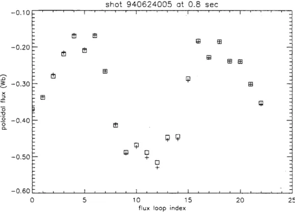
2-1 Flux at different flux loops due to the plasma alone (squares) and due to a filament carrying a current equal to the total plasma current and placed at the plasma current centroid location (crosses) for an elongated Alcator C-Mod shot. . . . . 40

2-2 Singular values of the matrix &Ag(p) normalized to the maximum one for an elongated Alcator C-Mod shot. Indices go from 0 to 12. 48

(10)

2-3 Flux contours for a typical equilibrium and locus E used for coil-to-vessel mapping (stars). . . . . 50

2-4 Quantities involved in the approximate edge flux conservation. . . . 53 2-5 Illustration of the convergence band of perturbation sizes. . . . . 57 3-1 Model of Alcator C-Mod. The boxes with a "+" sign represent

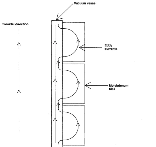
toroidally continuous elements. The empty boxes represent toroidally discontinuous elements that were left out of the model. . . . . 65 3-2 Illustration of effective toroidal current path due to the molybdenum

tiles. . . . . 66

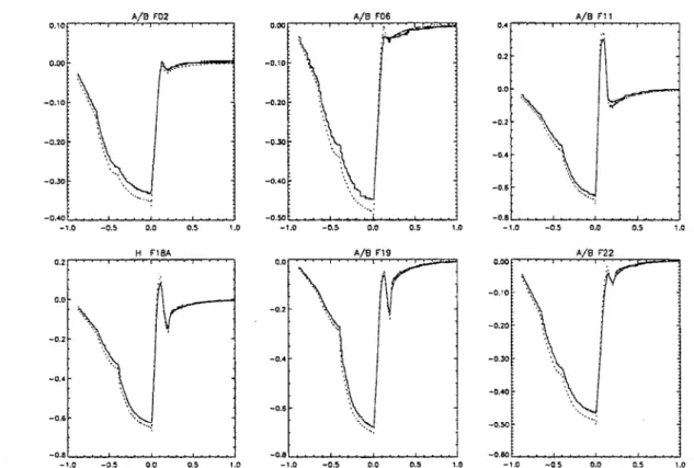
3-3 Comparison between flux loop signals (solid line) and their values as estimated from the measurements of the currents flowing in the coils using the 190-element model of the vessel and structure (dotted line). 70

3-4 Comparison between Br-coil signals (solid line) and their values as estimated from the measurements of the currents flowing in the coils

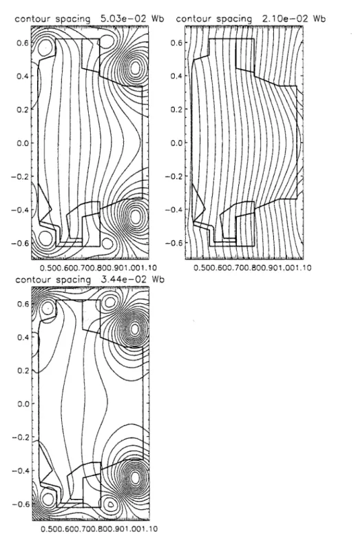
using the 190-element structure/vessel model (dotted line). . . . . . 71 3-5 Poloidal flux due to the active coil currents (top left), passive currents

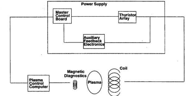
(top right), and both (bottom) 50 msec after breakdown. . . . . 73 3-6 Block diagram of the power supply and its position in the plasma

control loop. . . . . 75 3-7 Demand versus output voltage for the OH2U power supply at a time

interval of near-zero demand for a shot where the internal control loop was broken (*, solid line fit) and for a similar shot where the internal control loop was closed (+, dotted line fit). . . . . .. . . . 76

(11)

3-8 OH2L power supply output voltage before breakdown as a function of time for a shot with proportional gain in the internal feedback loop (top) compared to a typical shot with integral gain in the internal feedback loop (bottom). . . . . 77 3-9 OH2U (left) and OH2L (right) power supply demand (top) and

out-put voltage (bottom) for one of the power supply characterization shots. The fast modulation (500 Hz) demand signal is aliased. . . . 79

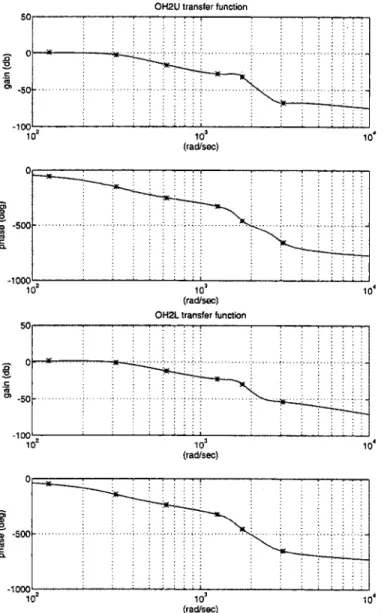
3-10 Bode plots for OH2U (top) and OH2L (bottom) power supply fitted

transfer functions. The measured points are shown as stars. . . . . 80

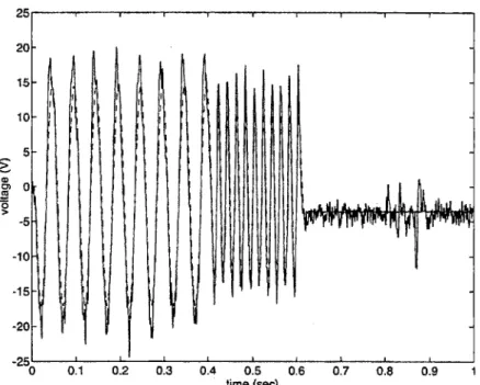
3-11 OH2L supply output voltage (solid) and simulated output voltage

(dotted) for one of the power supply characterization shots. The simulated output was calculated using the fitted transfer function. . 81

3-12 Comparison of the measured OH2U transfer function to the

compos-ite closed-loop transfer function consisting of individually measured transfer functions of the master control board, the SCR array (top only), and the auxiliary feedback electronics. . . . . 82

3-13 Traces characteristic of the vertical oscillation. The top two traces

show the difference in demand and output between upper and lower OH2 power supplies The bottom trace is the position of the plasma current centroid as calculated from soft X-ray tomography measure-m ents. . . . . 83

3-14 OH2U supply transfer function taking into account the proportional gain in the internal control loop. . . . . 84

3-15 Bode plots for the EFC power supply fitted transfer function. The

(12)

3-16 Bode plots for EF1U (top) and EF1L (bottom) power supply fitted

3-17 Bode plots for EF2U (top) and EF2L (bottom) power supply fitted

4-1 c,(w) for two different model reduction methods. The two models reduced by Hankel singular mode decomposition are of length 10 (upper) and 40 (lower). The unstable mode eigenvalue is reproduced exactly in all cases. . . . . 101

4-2 Er(w) for eigenmode decomposition. . . . . 103

4-3 c,(w) for Hankel singular mode decomposition. . . . . 104

4-4 c, at 10 Hz as a function of number of modes kept for eigenmode (eigen) and Hankel singular mode (HSM) reduction of the composite vessel/structure system with and without a generic plasma. . . . . . 105

4-5 Difference between reduced model and full model unstable eigenvalue

(279.1 rad/sec) as a function of number of modes kept for eigenmode

(eigen) and Hankel singular mode (HSM) reduction of the composite vessel/structure system with and without a generic plasma. . . . . . 106

4-6 E, at 10 Hz as a function of number of vessel modes kept in addition to 10 structure modes for eigenmode (eigen) and Hankel singular mode (HSM) reduction of the separate 96-element vessel/ 94-element structure with and without a generic plasma. . . . . 107

4-7 Difference between reduced model and full model unstable eigenvalue

(279.1 rad/sec) as a function of number of vessel modes kept in

addi-tion to 10 structure modes for eigenmode (eigen) and Hankel singular mode (HSM) reduction of the separate 96-element vessel/ 94-element structure with and without a generic plasma. . . . . 108

(13)

5-1 Comparison between actual poloidal flux measurements (+), predic-tions from EFIT (box), and the circuit equation/free boundary code com bination (*). . . . . 113

5-2 Current density in the passive conductor elements and poloidal flux due to the passive conductor currents as they are estimated using EFIT. The sign in each element indicates current direction. . . . . . 115

5-3 Current density in the passive conductor elements and poloidal flux due to the passive conductor currents as they are estimated using the circuit equation. The sign in each element indicates current direction. 116

5-4 Normalized conductor current density corresponding to the eigen-vector of the open-loop unstable eigenmode of a typical elongated plasma. The sign in each element indicates current direction. The flux due to these currents is also shown. . . . . 118

5-5 Traces characteristic of the shots where the feedback was turned off to observe plasma behavior. Shown are the R- and Z-location of the plasma current centroid (top two plots), the total plasma cur-rent (second from bottom), and the proportional gain in one of the feedback channels (bottom). . . . . 120

5-6 Characteristic jump in the EFC current when the feedback is turned

off. Also shown is the demand to the EFC power supply and the Z-position of the plasma current centroid. The feedback is turned off at 0.75 sec. . . . . 122

5-7 Experimentally observed rise in the Z-position of the current

cen-troid during the 10 msec of turning off of the feedback is fitted to an exponential in order to be compared to theoretical growth rate predictions. . . . . 123

(14)

5-8 Theoretically predicted vs experimentally observed growth rates. Stars

and diamonds denote growth rates calculated using the perturbed equilibrium model and the filament model respectively. . . . . 125

6-1 The subsystems of the closed loop. . . . . 128

6-2 Z-position traces of the plasma current centroid as calculated from

soft X-ray tomography measurements for three shots from the day when integral gain was applied for the first time. . . . . 133

6-3 Traces characteristic of the vertical oscillation. The top trace shows

the plasma current. The bottom two traces show the Z- and R-position of the plasma current centroid as calculated from soft X-ray tomography measurements. . . . . 135

6-4 Flux created by the eigenvector of the vertical mode by itself (left) and overlaid on the plasma equilibrium flux (right). . . . . 136

6-5 Root locus of the vertical mode (top) and the

OH2

power supply mode (bottom) when the EFC controller gain is varied. . . . . 138

6-6 Root locus of the vertical mode when the OH2 controller gain is varied. 139

6-7 Root locus of an OH2 power supply mode when the OH2 controller gain is varied. . . . . 139

6-8 Flux created by the eigenvector of one of the OH2 modes by itself (left) and overlaid on the plasma equilibrium flux (right). . . . . 140

6-9 Z-position of the plasma current centroid as calculated from soft

X-ray tomography measurements for two shots with different derivative gain in the fast Z-position control channel. . . . . 141

6-10 Characteristic traces from a shot with steps in the prescribed

(15)

6-11 Simplistic picture of a"filament plasma" in the presence of the vertical

field created by the EFC coils. . . . . 146

6-12 Z-position trace during a step change (solid line) and fit to the initial

behavior (dotted line). . . . . 149

6-13 Comparison of theoretical to experimental closed-loop growth rates

for the ten cases considered in this chapter. The lines through the origin of slope 1/2, 1, 2, and 3 are shown . . . . 150

6-14 Comparison of theoretical to experimental closed-loop oscillation frequencies for the ten cases considered in this chapter. The lines through the origin of slope 1/2 and 1 are shown. . . . . 151

6-15 Root locus of one EFC power supply mode (triangles), one OH2

power supply mode (diamonds), and the vertical mode (stars) as controller gain to the EFC power supply is varied from zero to five. 152

6-16 Root locus of the vertical mode as controller gain to the EFC power

supply is varied from zero to five neglecting all power supply dynamics. 152

6-17 Root locus of one EFC power supply mode (triangles), one OH2

power supply mode (diamonds), and the vertical mode (stars) as controller gain to the EFC power supply is varied from zero to five. This is shot 930923019 with fast Z-control derivative gain from shot 940624005. . . . .. . . . . 154

6-18 Z-position of the plasma current centroid (top) and demand signal

(bottom) to the EFC power supply showing the saturation effect. . 155 6-19 Vertical position after a step as measured (dotted), and as calculated

(16)

6-20 Demand signal to the EFC power supply after a step as measured

(dotted), and as calculated by means of a linear (dashed) and a non-linear (solid) simulation. . . .. . . . 158

6-21 Comparison of theoretical to experimental closed-loop growth rates

for the ten cases considered in this chapter. The line through the origin of slope one is shown. Theoretical growth rates were derived from the nonlinear evolution. . . . . 160

6-22 Comparison of theoretical to experimental closed-loop oscillation

fre-quencies for the ten cases considered in this chapter. The line through the origin of slope one is shown. Theoretical oscillation frequencies were derived from the nonlinear evolution. . . . . 161

7-1 Implementation of the step in the reference I, Z, using one channel (top) and two channels (bottom). . . . . 172

(17)

List of Tables

3.1 OH2L gain and phase data for some shots with oscillations. . . ... 83

4.1 Essential characteristics of the example and generic equilibria used in this section. . . . . 100

5.1 Growth rates in sec-1 for some shots where the feedback was turned off. . . . . 124

6.1 Feedback gains applied to the slow Z-position control channel for

three cases. . . . . 134

6.2 Open-loop growth rates calculated theoretically for ten cases with

step perturbations. . . . . 148

6.3 Comparison of theoretical to experimental closed-loop eigenvalues for the ten cases considered in this chapter . . . . 148

(18)

Chapter 1 Introduction

1.1 General Background

The concept of magnetic plasma confinement relies on the fact that charged particles are constrained to gyrate around magnetic field lines making it difficult for them to move perpendicularly to the magnetic field. Since motion along the magnetic field is free, one wants to close the magnetic field lines onto themselves or have them lie on a closed surface within the confinement device, thereby preventing the particles from leaving it. In the tokamak, see Fig. 1-1, this is achieved by bending a tube of magnetic field lines into a torus. The magnetic field is mainly in the toroidal direction, but there is a smaller poloidal component created by the current flowing toroidally in the plasma. This current is necessary to complete the confinement configuration.

One can follow the equations of motion of single particles and arrive via ensem-ble averaging at a set of kinetic equations for the distribution function over space and velocity of each species in the plasma. These are known as the Boltzmann equations, which, together with Maxwell's equations, are a complete description, provided one knows the effect of collisions on the distribution function.

(19)

Ideal magnetohydrodynamics (MHD) is a fluid model to describe certain basic macroscopic equilibrium and stability phenomena in a plasma. It results after taking velocity moments of the Boltzmann-Maxwell equations and rests on the following three assumptions:

* we are dealing with plasmas with thermal velocities much smaller than the speed of light and phenomena with phase velocities much smaller than the speed of light, so that the displacement current in Ampere's equation can be neglected.

* electron inertia is negligible, so that electrons respond quickly enough to cancel any charge imbalance and the net charge in Poisson's equation is zero. This is known as the quasineutrality condition. This assumption also implies that we are dealing with slow phenomena.

* the plasma is so dominated by collisions that it can be described by a scalar, isotropic pressure.

The first two assumptions are well justified for fusion plasmas for most macro-scopic phenomena of interest and lead to a set of single fluid equations. The third assumption is not always justified for fusion plasmas, but, it turns out that many macroscopic phenomena of interest are not dependent on the evolution of the pres-sure tensor. The ideal MHD equations can be summarized as:

The continuity equation:

= -pV -(

where p is the plasma density and Y is the fluid velocity. The momentum equation:

(20)

where J is the plasma current density and B is the magnetic field. The state equation:

(d) pV (1.3)

where y = 5/3.

Ohm's law:

E + vxB = 0 (1.4)

All the above quantities are functions of space and time, and d = a + -V is the

Lagrangean derivative.

In steady state, the momentum equation says that the Lorentz force is balanced everywhere by the pressure gradient. If we define the poloidal flux, O(R, Z) as the

total magnetic flux flowing through a horizontal circular loop of radius R centered at the tokamak axis at a distance Z from the midplane, the magnetic field can be written in terms of this flux and, using Ampere's law, the momentum balance equation can be rewritten as:

(V4' dp d

R2_V_- _{- -poR} 2 _- _F(1.5)

R2 dO dO

where F = RB4, and B4. is the toroidal field. Eq. 1.5 is known as the Grad-Shafranov equation describing axisymmetric toroidal plasma equilibrium. Note that F and the pressure are functions of

4

alone, i.e., they are constant on contours of constant poloidal flux. Also note that the right hand side in Eq. 1.5 can be written as -RJO(V)) where J4 is the toroidal plasma current. Given p(o) and F(0) profiles and a set of external currents, Eq. 1.5 determines the shape of the flux contours. For the plasma area, these are usually closed concentric contours. The innermost contour is known as the magnetic axis of the plasma.

Linearized MHD stability can be studied when we consider perturbations from an equilibrium with zero fluid velocity

(6

= 0). All perturbed quantities can be

(21)

velocity, V:

()

When the equilibrium is toroidally symmetric, this can be expressed as a sum of normal modes by writing:

(5, t) = o(r, 0) exp (inO + iwt) (1.6)

where n is the toroidal number of the mode. Definitions of the spatial coordinates are given in Fig. 1-1. The plasma is stable if the imaginary part of the eigenvalue, w, is non-negative for all modes of the system. Instability can arise from pressure gradients or from current flowing parallel to the field.

The advantages of the tokamak over other magnetic confinement schemes for controlled nuclear fusion have always been shadowed by the fact that the maximum

Pt allowable for magnetohydrodynamic (MHD) stability is low. Being the ratio of plasma to magnetic pressure, Ot is a measure of performance over cost and is directly related to how suitable a confinement scheme is for efficient power gen-eration. This limit arises from the so-called ballooning modes and external kink modes. Ballooning modes are high-n pressure-driven modes due to the unfavor-able field curvature characteristic of a tokamak. Kink modes can be driven either

by pressure gradients or by the current, and they dictate limits both on /3 and

total plasma current. Overall field stability can be made favorable by shaping the plasma cross-section. It has been shown, both theoretically and experimentally in the past ten years [1, 2, 3, 4, 5], that, elongation and triangularity of the plasma cross-section, allows for a higher plasma current which improves MHD ft-limits and confinement. For this reason, most tokamaks built in the 1980's and 1990's have shaped plasma cross-sections. Examples are: JET in the U.K., ASDEX-U in Germany, JT-60U in Japan, DIII-D, Alcator C-Mod, and PBX-M in the U.S.A., and TCV in Switzerland. Note that, except for JET, all other experiments are suc-cessors to or modifications of circular cross-section tokamaks that existed previously in the same research centers.

(22)

Br r R r :minxrtim R :njrraU Bt :brd"W Jp :pbMawMt B :polidWfidd ( :kwddalanijle 0 :pddcdalang*

Figure 1-1: Tokamak geometry.

(23)

Shot 940624003 @ 0.12 sec Flux contour spacing (L/R): 0.058Wb/0.012Wb 0.4-0.2 0.0 -0.2 -0.4--0.6 0.500.600.700.800901.001.10 0.500.600.700.800.901 .001.10

Figure 1-2: Poloidal flux contours without (left) and with (right) the plasma at a time early in the shot when the plasma is not strongly shaped yet. The right plot shows only flux surfaces inside the plasma.

0.6 0.4 0.2 0.0 -0.2 -0.4 -0.6

(24)

special attention since they represent global motion of the plasma, usually toward the vacuum vessel wall. The most dangerous of these is the so-called vertical insta-bility, which is an almost rigid vertical shift of the plasma and is always associated with strong shaping of the plasma. In order to create an elongated plasma, one has to use the poloidal field coils to pull the plasma from the top and bottom and push it from the sides. This is essentially a quadrapole field that has to be superimposed on the vertical field, which is necessary to balance the forces that push the plasma outwards in the radial direction [6]. These are: 1) the tire tube force due to the fact that the plasma pressure is constant on surfaces that have a smaller inboard area than outboard area and 2) the hoop force due to the fact that the force from both toroidal and poloidal magnetic pressure is larger on the inboard side. The externally applied poloidal field can then be concave towards the outboard side, whereas for a plasma of circular cross-section plasma it is approximately straight. This is shown in Figs. 1-2 and 1-3. Fig. 1-2 shows the magnetic field due to the coils and the structure alone at the beginning of a typical Alcator C-Mod discharge shot. This is the time right after breakdown and the plasma has not been shaped yet. It is still nearly circular and the vacuum field needed for equilibrium is purely vertical or concave towards the inboard side over a large region. Fig. 1-3 shows the magnetic field due to the coils and the structure alone at a time later in the shot, when the plasma has been given an elongated, triangular shape. Note how a larger part of the field lines are now convex towards the inboard side. Fig. 1-4 shows schematically how the vertical instability can arise. If the plasma current flows into the page, the equilibrium field has to be pointing downwards in order to create an inward force and balance the toroidal expansion forces. Imagine the plasma current being concentrated in one toroidal filament. At equilibrium, the filament sits on the midplane and sees no radial externally applied magnetic field. Now, if the field is convex towards the inboard side, and the filament moves off the midplane down-wards, it sees an outward radial field, which creates a downward force, pulling the

(25)

filament even further away from equilibrium. In the absence of a conducting wall around the plasma, the timescale of this instability is of the order characteristic of most MHD phenomena, known as the Alfven timescale. For a 1 keV ion tempera-ture, and a 1 m length scale this timescale is in the psec range. With a conducting wall around the plasma, the induced eddy currents provide damping and bring the instability timescale to the order of the skin penetration time of the conductor.

Shot 940624003 @ 0.8 sec Flux contour spacing (L/R): 0.096Wb/0.025Wb

0.6 0.4- 0.2-0.0 -0.2 -0.4 -0.6 0.6 0.4 0.2 0.0 -0.2 -0.4 -0.6 0.500.600.700.800.901.001.10 0.500.600.700.800.901.001.10

Figure 1-3: Poloidal flux contours without (left) and with (right) the plasma at a time later in the shot when the plasma is elongated. The right plot shows only flux surfaces inside the separatrix.

In the earlier tokamaks, where the duration of the plasma discharge was not considerably longer than the skin penetration time of the vacuum vessel, the vessel acted as a perfect conductor, stabilizing these modes, so that controlling them was not necessary. Modern tokamaks, though, have discharges with a duration tens or hundreds of times longer than the L/R time of the vacuum vessel. It is of utmost importance that the vertical instability is kept under control. When vertical control

(26)

is lost, the plasma moves up or down until it hits the vessel and is extinguished. This is known as a disruption. The eddy currents that are induced in the vessel during a disruption exert very large forces on the vessel, and for most high perfor-mance tokamaks these forces may threaten the mechanical integrity. In a reactor relevant tokamak like the proposed International Thermonuclear Experimental Re-actor (ITER) [7], the plasma will have enough thermal energy to vaporize 40 kg of Beryllium, one of the plasma facing materials being considered. In case of such an accident, the reactor might have to be shut down for a long time to repair the first wall.

p x Bz - FR

J p x BR - Fz

B

Figure 1-4: Interaction of a toroidal current with a curved equilibrium field.

1.2 Related Work

As mentioned earlier, there are several other tokamaks in operation in the world with shaped plasma cross-section and they all have to deal with the problem of the vertical instability. Consequently, a lot of work has been done so far in this field.

(27)

In the older configuration of JET, instability growth rates of 50-150 s- were observed [8]. A single-filament plasma representation was used together with two circuit equations, one for the vertical control coil pair and one for the vacuum vessel.

By choosing appropriate values for the parameters of this model, the open loop

growth rates were reproduced satisfactorily [9]. In voltage step tests, the oscillation frequencies and growth rates were predicted to within a factor of two [9, 10]. Nothing has been published yet on the new configuration. The modeling of the growth rates for the vertical instability is unresolved, in the sense that they do have large discrepancies between predicted and measured growth rates for divertor plasma configurations [11].

For DIII-D vertical stability analysis so far, the plasma has also been modeled as a single filament [12]. Its inductance is not allowed to vary with Z. The vacuum vessel is constrained to have one antisymmetric poloidal distribution of toroidal currents. Finite resistivity is allowed for the vacuum vessel and the control coil pair. The equation of motion for the massless single-filament plasma (which is equivalent to BR = 0 at the filament location) together with the circuit equations for the

vessel and the control coil pair give a third order system. From these equations, it becomes clear that, without feedback, the plasma becomes vertically unstable on an MHD timescale, when the decay index becomes smaller than a critical decay index defined by

2Ro _aM, _2(1.7)

where Mp is the mutual inductance between the plasma filament and the vacuum vessel, L, is the self-inductance of the vessel, RO is the radial location of the plasma filament and

Le t

4±

+ + (1.8)

poRo 2 2

Let and 1j are the external inductance and internal inductivity of the plasma re-spectively. This model was used as guidance when exploring the stable operating space of feedback gains. In Ref. [13], this model was tested against experiments

(28)

where the plasma was moved up and down by means of steps in the voltage ap-plied to the coil pair controlling the vertical position. The order of the response was confirmed, as was the maximum achievable decay index. The growth rates and oscillation frequencies of the modes of response, however, could only be predicted to within a factor of two of the observed ones, if one unjustifiably adjusted the vessel resistance by 50% and multiplied the actual feedback gains used by a factor of four. No experiments were conducted, in which feedback control was turned off, while the plasma was unstable. This experiment can result in a disruption, so that a large number of them can be damaging to the tokamak. This is why it is usually avoided. It is, however, the only direct way to compare open loop plasma behavior to theory. Perturbed equilibrium modeling of the plasma has also been done [14], but has not been experimentally validated yet.

ASDEX-U differs from other machines in the method used to interpret the

magnetic measurements in order to infer the state of the plasma. A large number of MHD equilibria have been computed and the values of all the measurements used

by the control system as well as the basic equilibrium parameters that are being fed

back on have been stored in a database [16]. Using function parametrization [17], a quadratic relationship between equilibrium parameters and measurements was developed. A simple filament model of the plasma, together with 6 modes for the vacuum vessel were used to produce rough estimates for feedback gains. The Tokamak Simulation Code (TSC) [18] was then used in place of the tokamak to test the control loop in pseudo-real time [19, 20]. TSC calculates the time evolution of a free-boundary plasma equilibrium, which is consistent with a prescribed sequence of currents in the poloidal field coils and the passive conductors. A better set of feedback gains is developed this way, which is ultimately tested on the tokamak itself. Substantial work has been done on electromagnetic modeling of the passive conductors in ASDEX-U [21, 22]. For no-plasma runs, the passive stabilizer loop current was predicted via 2-D eddy current modeling to within a 30% accuracy,

(29)

while in plasma runs, 2-D eddy current modeling with a filament model of the plasma reproduced flux loop measurements to within a 20-50% accuracy.

As in ASDEX-U, in TCV control laws are being tested using TSC [23, 24]. The NOVA-W code [25] is also used to assess the effect of plasma deformability on closed loop axisymmetric response. NOVA-W is a linear MHD stability code which takes the effects of resistive conductors in the vacuum region into account. The passive eigenmode always rearranges itself under active feedback so that the flux measurements used in the feedback loop are minimized [26], thereby minimizing the effect of the feedback system. NOVA-W was used to determine which measurements and which actuators (PF coils) to weigh more heavily for more effective control. A similar approach is also used in PBX-M [27].

In JT60-U a rigid multifilament model of the plasma was used together with a vacuum vessel modeled as a set of 100 toroidal conductors [29]. In experiments where feedback was turned off during vertically stable discharges, the theory predicted the Z-evolution very well. In closed loop experiments where the plasma was perturbed

by means of neutral beam injection, the growth rate was predicted accurately, and

the oscillation frequency to within a factor of three.

A survey of related work performed so far shows that several sophisticated

models exist for the axisymmetric motion of a plasma in the presence of resistive conductors. These models are used in a trial-and--error mode as an aid to finding good feedback laws. However, these models have not been used substantially in the context of linear control theory, to derive control laws, or predict experimen-tal behavior. Only very simple models have actually been used for this purpose.

(30)

1.3 Alcator C-Mod

Alcator C-Mod is the third in a series of compact, high-field tokamaks built at M.I.T. and aimed at achieving high performance at low cost. Unlike its predeces-sors, it has an elongated vacuum vessel, and the poloidal field (PF) coils are located inside of the toroidal field (TF) coils. In addition, it features ten independent power supplies feeding a set of 13 PF and ohmic heating (OH) coils. It has, therefore, the capability of producing a large variety of shaped plasmas, and divertor configura-tions. Fig. 1-5 shows a cross-sectional view of Alcator C-Mod. It can have a

VERTICAL PORTS ,20OLES

DRAW BAR 10,560LBS

NUTS 1,250LBS

UPPER COVER 57,680LBS DOWEL PINS 670LDS

LOCK PINS L150LBS

UPPER WEDGE PLATE 10,750LBS

CYLINDER 44,000LBS EF-el MOUNTING BRACKETS aIIO0LBS

(I0) F COILS IDDO00tES

PLASMA 0.DTDDLBS

tiles 4,83tbs

TAPERED PINS 6SOLDS

LOCK SCRES 4 LBS LOWER VEDGE PLATE I0,75DLBS

LOVER COVER 57,68LDS

CRYOSTAT 5,060LBS

VERTICAL PORT FLANGES 200LBS

OH COIL 3,000LBS TF MAGNET 48,000LBS

MOUNTING PLATE-TOP D800LBS

HORIZONTAL PORTS 500LBS

HORIZONTAL PORT EXTENTIONS F7 HORIZONTAL PORT FLANGES 31

VACUUM OHAMBER 6LANGLBS

MOUNTING PLATE-BOTTOM F800LBS DCL BS 00LES

Figure 1-5: Cross-section of Alcator C-Mod

(31)

-EF2U _EF3U EFCU EFCL - EF2LEF3L * FL EF1 U OH2U

7-Figure 1-6: Cross-section of the vacuum vessel showing the OH and PF coils.

toroidal current of 3 MA. All magnets are made of copper and cooled with liquid ni-trogen. Fig. 1-6 shows a closer view of the coils. Power is supplied by an alternator, connected to a flywheel capable of storing 2000 MJ of energy.

The main function of the OHI coil is to control the toroidal loop voltage (and hence the total plasma current) by varying the time derivative of the poloidal flux. The difference between OH2U and OH2L currents controls the Z-position of the plasma on a slow timescale, while the EFC coils, which are connected in antiseries, control the Z-position on a faster timescale. The OH2 coils are fed by

two powerful but slow power supplies, while the EFC coils are fed by a smaller but faster power supply. The R-position of the plasma is mainly controlled by the EF3 coils connected in series, which are fed by one power supply. Alcator C-Mod is mostly run in a so-called diverted, single-null configuration. This means that the last closed surface of constant poloidal flux (separatrix) does not touch the vacuum

II II II ii I I -~ I \ \ OH2L EF L EF4U TF magnet leg

I

- Outer cylinder ---- _{Cryogenic dewar} EF4L OH1 i

(32)

vessel wall (see Fig. 1-3) and that the two points of zero poloidal field that form outside the last closed flux surface (x-points) are not symmetric; one of them is further away from the plasma than the other, so that most of the particles escaping the plasma by means of perpendicular (to the field lines) transport, end up through parallel transport at one end of the vacuum vessel. The Z-position of the x-points is mainly controlled by the EF1 coils. The EF2 coils control the x-point R-position. The sum of the OH2 coil currents together with the EF4 coils, which are connected in series, control the elongation and triangularity of the plasma by pushing on it from the outside and pulling on it from the inside.

The control of individual plasma shape and position parameters is actually much more coupled than this simplistic one-to-one identification of coil functions, however, and necessitates the use of a very flexible control system. Fig. 1-7 shows a block diagram of the hybrid digital/analog plasma control computer system used in Alcator C-Mod. It can take up to 96 signals as input. The interpretation of the state of the plasma is done by multiplying these signals by a predictor (A,-matrix) to form up to 16 different linear combinations representing the parameters to be controlled. These signals are then compared to their pre-programmed values and the error, its integral and derivative are then multiplied by some gains. The result-ing 16 signals are then multiplied by the controller (M-matrix) which determines what coils are to be involved in controlling each parameter. The pre-programmed voltage demand signals determine the general scenario of the discharge. They are added to the output of the controller and the sum goes to the power supplies as voltage demand. All matrix multiplications are performed in an analog way, but the matrices are inserted digitally and can be changed during the discharge.

The inputs to the plasma control computer are mainly magnetic diagnostic measurements of two types: poloidal magnetic flux and poloidal magnetic field on the inside surface of the vacuum vessel. The poloidal flux is measured by the so-called flux loops. These are wires running toroidally along the vacuum vessel wall.

(33)

M matrix 16 16 0 n t r 0 pre-programmed values _e of parameters to be r controlled one P I D of 16

Q

summer 96 A matrix p r e d C tr 0 r 16 pre-programmed voltage demands

V

1+ +0 + summers power supplies coils plasma a 9 n 0 s t C 5

(34)

The principle of operation in demonstrated in Fig. 1-8. The area A is large and the

B

V

Integrator>

Figure 1-8: Illustration of the principle of operation of the flux loops.

magnetic field B going through it is in general toroidally nonuniform. The output V is then

V dOp d

d tJ ds (1.9)

This is a toroidally averaged measurement, except for some loops that do not go all the way around toroidally, but are located on the vacuum vessel wall between two ports (partial flux loops). The poloidal magnetic field is measured by the B,-coils. These are small pick-up loops located at different poloidal locations, oriented so that no toroidal field flows through them. They operate on the same principle as the flux loop, the difference being that the area A is small enough that the magnetic field i

(35)

going through it can be considered uniform. The output V then is proportional to

. This is therefore a localized measurement. There are 21 full flux loops, 6 partial flux loops and four sets of 26 Bp-coils located at four different toroidal locations.

The vacuum vessel, which has some sections as thick as 2 cm, serves also as structural support for the PF coils and the first wall hardware. A large amount of stainless steel serves as structural support for the TF coils. Both the vacuum vessel and the structure are toroidally continuous for the most part and can carry large eddy currents; this is desirable for passive control, because it helps slow down any unstable axisymmetric plasma behavior. However, it also means that active control is slower, since any change in the coil currents (which are outside the vacuum vessel) creates eddy currents in the vacuum vessel and can only create a change in flux inside the vacuum vessel after the eddy currents have died away. The first wall consists of molybdenum tiles, and the bottom of the vacuum vessel is fitted with a closed, baffled divertor chamber.

Auxiliary plasma heating is provided by two transmitters supplying a total of 4 MW of ion cyclotron radio frequency waves. Because of its high particle-, power-, and current- densities, Alcator C-Mod is expected to have edge plasma conditions that resemble those expected in ITER, and is therefore going to offer valuable information for the design of the ITER-divertor.

1.4 Motivation and Outline

From the above it is clear that vertical position control is essential for shaped toka-maks. So far, tokamaks have been controlled by simple proportional, integral and derivative feedback control that assumes that control of different plasma parame-ters is completely uncoupled; in other words each coil set affects only one of the parameters to be controlled. The advantage of this approach is that no model is

(36)

needed for the response of the unstable system we are trying to control. Instead, the "optimal" feedback gains are determined by trial and error from shot to shot.

If the no-coupling assumption is not true, however, the control of two different

plasma parameters will often cause two coil sets to fight each other, resulting in a non-optimal use of resources (voltage sources for the coils). This is due to the fact that changing one parameter may result in an undesirable change in another parameter. Modern control theory has many interesting methods to offer for good control of many-input many-output (MIMO) systems. When the control system of the tokamak is frequency independent (as is the case in Alcator C-Mod), optimal control theory can be used to make the most efficient use of the resources for the smallest possible deviation of certain plasma parameters from their desired values. With a frequency dependent controller, more sophisticated methods can be used to reduce the effect of noise (H,-theory) and structured uncertainties in the form of modeling errors and perturbations (p-synthesis theory). In both cases, however, a good linear model of system response is needed. During a typical shot the plasma goes through many different shapes and one cannot expect a single linear model to be valid for all cases. Control laws based on different models can be used during different phases of the plasma discharge. Most modern control systems (including the Alcator C-Mod control computer) have this capability which is known as "gain scheduling".

The purpose of this thesis is to examine the usefulness of linear axisymmetric plasma response models in predicting the behavior of Alcator C-Mod geometric shaping parameters and developing feedback laws to control them. In particular, it attempts to go one step beyond what has already been done in that it uses a more sophisticated plasma response model for this purpose than the single-filament or multifilament models that have been compared to experiment to a limited extent so far. The approach is to first create models for all the individual systems shown in

(37)

the closed-loop. Testing of individual systems in an open-loop configuration was very satisfactory, proving that the perturbed equilibrium plasma response model and a toroidally symmetric electromagnetic model of the vacuum vessel and the structure can be trusted for the purpose of calculations for control law design. Closing the loop introduced some serious nonlinearities making comparison of linear theory to experiment unsatisfactory. When these nonlinearities are added to the linear models, however, the experimentally observed behavior can be predicted by theory satisfactorily.

Chapter 2 will present two plasma response models. The first is the rigid multifilament model where the plasma is modeled as a set of toroidal filaments that do not move with respect to each other and whose current does not change. The second is the perturbed equilibrium model, namely a model that assumes that the plasma is always in a self consistent MHD equilibrium in the vicinity of some central equilibrium and that the time response is dictated by the L/R time of the conductors around it. Both of these models neglect plasma inertia. Chapter 3 presents an electromagnetic model of the vacuum vessel and the structure of Alcator C-Mod and how this model agrees with experimental measurements. This model is useful in plasma equilibrium reconstruction and was of some help in developing a repeatable plasma startup procedure. Models have also been developed for the power supplies that feed the equilibrium field coils and the results are also presented in Chapter 3. Chapter 4 develops a dependable way of reducing the order of the resulting models so they can be used for repeated time consuming control calculations. Chapter 5 presents a comparison of theory to experiment for elongated plasma discharges where the feedback control was turned off and the plasma moved exponentially towards the vessel wall. Chapter 6 presents a comparison of theory to experiment for elongated plasma discharges with the feedback loop closed. Finally, Chapter 7 presents a summary and conclusions that can be derived from the comparison of theory to experiment and suggestions for further work.

(38)

Chapter 2 Linear Plasma Response Models

2.1 General Assumptions

In order to exploit the many recent achievements of MIMO linear state space control theory, we have to have a linearized model for the response of the system consisting of the plasma and the conductors around it. To arrive at such a model several assumptions must be made. If the only tools we have to control the plasma are the OH and PF coils, we can only affect toroidally symmetric modes of the plasma, so we are justified in confining ourselves to considering axisymmetric behavior. If we suppose that the response of the plasma is governed by the ideal MHD momentum equation (Eq. 1.2), two timescales are of interest: the Alfv6n timescale of the plasma and the L/R timescale of the conductors around it. If the first is much shorter than the second (and usually it is by about 3 orders of magnitude), we are justified in

neglecting the inertia term in the momentum equation. The presence of the con-ductors slows down any instability from the Alfv~n timescale to the L/R timescale.

If the plasma were surrounded by a perfectly conducting vacuum vessel, it would be

stable. We are also justified in neglecting plasma inertia effects for a practical rea-son: the fastest Alcator C-Mod power supply cannot react faster than a timescale of

(39)

approximately 1-msec, so that if the plasma were unstable on the Alfv6n timescale, we would not be able to control it anyway. Then, the plasma is supposed to be in equilibrium at each time and the conductors determine how it moves from one equilibrium to the next. This is known as the quasistatic approximation.

A set of toroidal conductors is governed by circuit equations which describe

the evolution of the poloidal flux at the locations of the conductors:

MI+ RI= V (2.1)

where M is the inductance matrix (including mutual and self inductances), R is the diagonal resistance matrix for the conductors, and

V

is the vector of voltages applied to the conductors; its only non-zero elements are the ones corresponding to the active conductors. The word "active" here refers to a conductor that is being fed by a voltage source (power supply) as are the coils.

I

is a vector containing the currents flowing in the conductors. We can choose the state of the plasma at each point in time to be described by the poloidal flux it creates at the conductor locations. Then, including a linearized plasma response would amount to adding to M some matrix X accounting for the coupling between conductors mediated by the plasma [32]:

MI+ XI + RI = V (2.2)

Here, X = , and

?kp

is the poloidal flux at the conductor locations due to plasma current alone.

I

is then the state vector of the plasma/conductor system.

Several linear models for the plasma have been devised, some of which will be discussed in the following sections. All these models amount to finding the matrix X. The simplest one is to replace the plasma by a single toroidal filament

[12]. The next step is to use several toroidal filaments for the plasma in order to simulate a distribution of toroidal current in the plasma [30]. One can also determine the linearized plasma response by perturbing the conductor currents that give a certain base equilibrium of interest and considering the plasma to be always

(40)

in an equilibrium which is a linear combination of the set of perturbed equilibria. This approach was introduced in Ref. [31] and was extended in Ref. [32] to include passive conductor response and approximate flux conservation. A more rigorous approach based on the energy principle (but still neglecting plasma inertia) is used in Ref. [33].

The aim of this thesis is not to evaluate these plasma models or to suggest a new one, but rather to make contact between these models and the observed behavior in the Alcator C-Mod tokamak. Only when we feel confident, that we can explain the experimental observations with some linear model, can we go ahead and make use of the wealth of existing modern control theory techniques.

2.2 The Rigid Filament Model

Representing the plasma as a single toroidal filament placed at the position of the plasma current centroid ([12, 34]) is the simplest approach to the problem of vertical stability. Fig. 2-1 shows a comparison of the poloidal flux at the locations of some magnetic diagnostics (flux loops) due to the plasma alone for an elongated Alcator C-Mod plasma and due to a filament carrying a current equal to the total plasma current and placed at the plasma current centroid location. The flux pattern at the vacuum vessel, where all the magnetic diagnostics are located, is similar in both cases. It has been argued ([12]), therefore, that the single filament model of the plasma is a satisfactory descriptor as far as the control problem is concerned. The distribution of the plasma current, has to have some effect on plasma response, however, for two reasons: first, when some of the plasma current is placed closer to the vacuum vessel, more eddy currents will be induced when the "plasma" moves than when all of the current is placed in the middle of the vacuum vessel; second, as some current is spread over areas of different external field curvature than that of the current centroid location, its stability characteristics have to change. If the

(41)

-0.10 -0.20 -0.30 -0.40 -0.50 -0.60 C shot 940624005 at 0.8 sec ---8 ₈ ::8 -0± 5 10 15

flux loop index

20 25

Figure 2-1: Flux at different flux loops due to the plasma alone (squares) and due to a filament carrying a current equal to the total plasma current and placed at the plasma current centroid location (crosses) for an elongated Alcator C-Mod shot.

0 0_

(42)

plasma response is affected, the control problem will be affected as well.

If we know the plasma current distribution, the next logical step is to represent

the plasma as a set of toroidal current carrying filaments with a current distribution resembling that of the plasma. We can assume that the filaments do not move with respect to each other and restrict motion to the vertical direction only. This is done in Ref. [30]. These are of course nonphysical restrictions, since there can be other non-rigid and not exactly vertical modes which require less energy and are, therefore, more unstable. It is not clear how one should go about specifying these modes without going into a full MHD analysis, however. The rigid vertical motion is a good approximation at least for the qualitative analysis of elongated plasma response. The circuit equations for the conductors around the filaments become:

M-- i-. N Pj +N

MI +RI + 1p ' + I,;Mp = V (2.3)

where:

M,3 is a vector containing the mutual inductances from the ith plasma filament to all the conductors,

4,p

is the current in the ith plasma filament,

z is the change in vertical position of the plasma filaments and

N is the number of plasma filaments.

One has to specify how the plasma filament currents change. One possible assumption is that the IJj's change so as to conserve the poloidal flux. This is a valid assumption for an ideal (non-resistive) plasma. Another possible assumption is to assume that the plasma filament currents do not change, conserving plasma

current density. This second assumption is of course easier to implement, since the jpi-term vanishes in Eq. 2.3. Furthermore, it has been shown [35], that a rigid constant current shift is never more stable or further from the exact energy minimizing MHD eigenmode than a rigid constant toroidal flux shift. It makes

(43)

sense, therefore, to use the constant plasma current assumption.

To determine z, we need the equation of motion of the plasma. There are two forces acting on the plasma:

* The force due to the eddy currents induced in the conductors around the

plasma:

Feddy dEmag (2.4)

z dz

where Emag is the magnetic energy stored in the conductor and filament system and e, is the unit vector in the vertical direction:

EM +1 (2.5)

3 3 1'iMV1

where Mpjj is the j'th element of vector Mi from Eq. 2.3.

M N M

Feddy =

9ZZI

[

Ia

13 = T(2.6)

3 1p . 3Z 26

where M is the number of conductors around the plasma and the superscript T stands for transpose.

* The Lorentz force due to the interaction of the plasma filament currents

with the radial magnetic field encountered as the plasma moves a distance z from its equilibrium position:

NLorentz B aBR

FLrt - E 2rIpi- IZ LZ (2.7)

BRi is the radial field at the location of filament i.

We have then:

d2

z

M =t- +

Fz(2.8)

where m is the plasma mass. In the quasistatic approximation, the left hand side of Eq. 2.8 is negligible and one can simply solve for z and substitute into Eq. 2.3. z is the position where the Lorentz force balances the force due to the eddy currents.

(44)

Then, in the sense of Eq. 2.2, the mutual inductance matrix of the conductors due to their coupling to the plasma is:

X = (_ Ia

59)7

(2.9)

Eqs. 2.2 and 2.9 describe the response of a massless filament plasma in the presence of passive conductors and active coils. Performing eigenmode analysis on Eq. 2.2 usually gives one unstable mode for elongated plasmas, which is the vertical mode.

The plasma current distribution may be obtained either from an MHD equilib-rium code, if we are interested in the response of a theoretical plasma equilibequilib-rium, or can be reconstructed from data from a real plasma discharge at a particular time. In the second case, an MHD equilibrium code has to be run anyway in order to look at other equilibrium quantities for other purposes. In either case, the spatial grid used by the equilibrium code can be used as locations of the plasma filaments. All results presented in Chapter 5 are calculated using a set of 65 x 65 filaments coin-ciding with the grid of an equilibrium code. This is purely a choice of convenience. The computational cost of using so many filaments was small, and any operation attempting to lump plasma current on that grid into a smaller number of filaments would probably have had some computational cost as well. Of course, such a large number of filaments is not necessary to reproduce current distribution effects. A study was done in Ref.

[30]

to determine how the number of filaments affects the growth rate of the vertical mode. It was found that the growth rate varied con-siderably with fewer than ten filaments, but converged to some value when ten or more filaments were used.

2.3 The Perturbed Equilibrium Model

The perturbed equilibrium model is described in Ref. [32]. In this section, an overview of the model is given. First we look at the current conserving perturbed

Axisymmetric control in Alcator C-Mod

Axisymmetric Control in Alcator C-Mod

Axisymmetric Control in Alcator C-Mod

by

GERASIMOS TINIOS

B.S., Nuclear Engineering, Rensselaer Polytechnic Institute (1985)

Submitted to the Department of Nuclear Engineering

in partial fulfillment of the requirements for the degree of

Doctor of Philosophy

at the

MASSACHUSETTS INSTITUTE OF TECHNOLOGY

January 1995

@

Massachusetts Institute of Technology 1995

Signature of Author ...

Department of Nuclear Engineering

January 18, 1995

Certified by ...

Certified by...

Ian H. Hutchinson

Professor, Department of Nuclear Engineering

Thesis Supervisor

Jeffrey P. Freidberg

Professor, Department of Nuclear Engineering

Thesis Reader

A ccepted by ...

Axisymmetric Control in Alcator C-Mod

by

GERASIMOS TINIOS

ABSTRACT

Acknowledgments

Contents

References

176

List of Figures

OH2

List of Tables

Chapter 1

Introduction

1.1

General Background

4

(6

()

1.2

Related Work

4±

1.3

Alcator C-Mod

I

Q

V

B

1.4

Motivation and Outline

Chapter 2

Linear Plasma Response Models

2.1

General Assumptions

V

I

?kp

I

2.2

The Rigid Filament Model

4,p

9ZZI

[

Ia

Fz(2.8)

59)7

[30]

2.3

The Perturbed Equilibrium Model