HAL Id: hal-00673148
https://hal.inria.fr/hal-00673148
Submitted on 22 Feb 2012
HAL is a multi-disciplinary open access
archive for the deposit and dissemination of
sci-entific research documents, whether they are
pub-lished or not. The documents may come from
teaching and research institutions in France or
abroad, or from public or private research centers.
L’archive ouverte pluridisciplinaire HAL, est
destinée au dépôt et à la diffusion de documents
scientifiques de niveau recherche, publiés ou non,
émanant des établissements d’enseignement et de
recherche français ou étrangers, des laboratoires
publics ou privés.
Distributed Monitoring with Collaborative Prediction
Dawei Feng, Cecile Germain-Renaud, Tristan Glatard
To cite this version:
Dawei Feng, Cecile Germain-Renaud, Tristan Glatard. Distributed Monitoring with Collaborative
Prediction. 12th IEEE International Symposium on Cluster, Cloud and Grid Computing (CCGrid’12),
May 2012, Ottawa, Canada. epub ahead of print. �hal-00673148�
Distributed Monitoring
with Collaborative Prediction
Dawei Feng
∗, C´ecile Germain-Renaud
∗, Tristan Glatard
†∗ Laboratoire de Recherche en Informatique, CNRS − Universit´e Paris-Sud 11 † CREATIS, CNRS − INSERM − Universit´e Lyon 1 − INSA Lyon
Abstract—Isolating users from the inevitable faults in large distributed systems is critical to Quality of Experience. We formulate the problem of probe selection for fault prediction based on end-to-end probing as a Collaborative Prediction (CP) problem. On an extensive experimental dataset from the EGI grid, the combination of the Maximum Margin Matrix Factor-ization approach to CP and Active Learning shows excellent performance, reducing the number of probes typically by 80% to 90%.
I. INTRODUCTION
The recent crash of the Amazon Cloud [1] highlighted the importance of timely discovery of failures in large scale distributed systems: a local, limited error may result in a global catastrophe. Thus a significant part of the software infras-tructure of large scale distributed systems, whether grids or clouds, collects information (monitoring) that will be exploited to discover (knowledge) if, where, and when the system is faulty.
This paper addresses the knowledge building step in the context of end-to-end probing as the class of monitoring techniques. In the end-to-end probing approach, a probe is a program launched from a reliable entry point (probe station), which tests the availability (and possibly performance, but this is outside the scope of this paper) of the components on its path. The only observables are the outcomes of the probes, which are binary: success or failure. For instance, a ping command would test the overall software stacks and network connectivity from the probe station to the target computer.
The motivating application comes from operations manage-ment in the European Grid Initiative (EGI). Challenged by a high fault rate, especially concerning data access, the Biomed Virtual Organization daily runs end-to-end probes to test the availability of all relations between its endpoints, namely Computing Elements (CEs) and Storage Elements (SEs). The objective of this paper is to minimize the number of probes for a given discovery performance target. The probe overhead budget can then be spent on more intelligible probes.
We addressed the probe minimization problem as an in-stance of the Collaborative Prediction (CP) problem: given a small number of probe results, how to infer the capacities for other (CE, SE) pairs for which no probe is launched. Srebro et al. [2] made a decisive advance in CP by proposing the Maximum Margin Matrix Factorization (MMMF) method, which makes the optimization problem both well-defined and tractable. This paper proposes three combinations of
probe selection methods with MMMF. Extensive experiments conducted on 51 instances of the full problem show that the number of probes can be reduced by more than 90%. This result goes well beyond the particular application: the fundamental hypothesis for CP is that a limited number of common and hidden factors root the outcomes, here success or failure; this hypothesis is reasonable in the context of large scale distributed systems, where the hidden causes are likely to be related to hardware failures and misconfiguration of middleware services shared by clusters of users.
The main contributions of this paper are twofold: • modelling probe-based fault prediction as a CP task; • experimental evidence that MMMF is an extremely
effi-cient strategy for fault prediction.
The datasets are available online at the Grid Observatory portal1 and make our experiments reproducible.
The rest of this paper is organized as follows. Section II presents the motivating application and discusses the general context of fault prediction and fault diagnosis; section III details the probe selection algorithms; the data, evaluation methodology and experimental results are presented is section IV; section V discusses related work, before the conclusion.
II. PROBLEMSTATEMENT A. Motivating application
The European Grid Infrastructure (EGI) enables access to computing resources for European researchers from all fields of science, including high energy physics, humanities, biology and more. The infrastructure federates some 350 sites world-wide, gathering more than 250,000 cores, which makes it the largest non-profit distributed system in the world. Hardware and software failures are intrinsic to such large-scale distributed systems. Resource availability in production is about 90%, and middleware such as gLite [3] , Globus [4] or ARC [5] cannot handle this without substantial human intervention. Access rights to EGI are primarily organized along the concept of Virtual Organization (VO), and each of the 200 VOs has to be specifically configured on its supporting sites, which adds complexity and introduces extra failures. User communities exploit two related strategies to cope with faults: overlay middleware such as DIRAC [6], DIANE [7], AliEn [8] and PaNDA [9] implements specific fault-tolerance strategies to isolate users from the vagaries
of the infrastructure; and monitoring identifies problems and quantifies performance w.r.t. quality-of-service agreements.
The target system of this work is the Biomed VO. Biomed has access to 256 Computing Elements (CEs) and 121 Storage Elements (SEs). Informally, CEs are shares of computing resources, implemented as queues of each site manager (e.g. PBS), and SEs are shares of storage resources; the formal definition is part of the Glue Information model [10]. Testing the availability of all CE-SE pairs is one of the most chal-lenging issues encountered daily by monitoring operators. The current method is brute force: it periodically launches a fully distributed all-pairs availability test, for a total of 29512 tests, multiplied by the number of capacities to test at each run. Human operators cannot handle so many results; in practice, only a few issues are reported, with questionable selection criteria. With CP, a massive reduction of the number of tests provides nearly similar availability evaluation performance, creating opportunities for better frequency/intrusiveness trade-off and selection of reported incidents.
B. Fault prediction and fault diagnosis
Minimizing the number of probes can be addressed along three avenues: fault prediction, detection and diagnosis. In all cases, the system under consideration is a set of hardware and software components, which can be functioning correctly (UP) or not (DOWN). These components feature some dependencies - e.g. a service certainly depends on the hardware it is running on, and possibly of other services. In the detection problem, the goal is to discover if any of the components is DOWN, while in the diagnosis problem, the goal is to exhibit all DOWN components. Both cases assume a priori knowledge of the components of the system, as well as knowledge of the dependency matrix, which describes the outcome of each probe given the status (UPorDOWN) of these components. For a given set of probes, diagnosis has linear complexity in the number of components; however, optimal probe selection is NP-hard for detection and diagnosis, because it is equivalent to the minimum cover set problem [11].
The obvious advantage of diagnosis (and to some extent detection) is that it provides an explanation of the failure, by exhibiting the culprits. On the other hand, it strongly relies on a priori knowledge - which components are required for a probe to succeed - through the dependency matrix. For massively distributed systems, where Lamport’s famous definition ”A distributed system is one in which the failure of a computer you didn’t even know existed can render your own computer unusable” applies, assuming such knowledge might be hazardous in principle. In our case, the very large scale of the dependency matrix, and its particular shape, mainly a block-diagonal structure, calls for further research in order to explore the typical multi-faults configurations.
Instead, this paper focuses on fault prediction. In this case, the overall infrastructure is a black box, with no a priori knowledge of its structure. The question is, given a small number of probe results, how to infer the capacities for other (CE, SE) pairs for which no probe is launched. In this
context, fault prediction can be considered as a case for CP. CP is originally a technique for predicting unknown ratings of products for a particular user, based on observed data from other users and products. It can be applied to various domains such as online recommendation, link prediction and distributed system management applications discussed in this paper. It is fundamentally a matrix completion task: given a very sparse users by products matrix, whose non-zero entries represent known ratings, predict the unknown entries of the matrix. The success of CP relies on the hypothesis of a factorial model: hidden and partially shared factors affect the matrix entries. For example, two nodes (CE or SE) may share several hidden factors - e.g. location, with the associated network connectivity issues, or use of a particular instance of any middleware service (e.g. brokering, authentication), such that the availability of the CE-SE relation may be affected similarly.
Optimal probe selection for fault prediction is NP-hard too: assume that the hidden factors have been identified by CP, and that we want to exhibit the optimal probe set, a posteriori. Then, the probe selection problem is equivalent to diagnosis, but with the factors as components.
III. GOALS AND METHODS
From the previous description, it follows that minimizing the number of probes encompasses two distinct issues.
• Probe selection: which subset of the (CE,SE) pairs will actually be tested?
• Prediction: predict the availability of all (CE,SE) pairs from a small number of them.
A. Probe selection
input : Initial partially observed binary(-1/+1) matrix M0, threshold λ, max # of new samples N , active-sampling heuristic h
output : Full binary-valued matrix MTi predicting
unobserved entries of M0 initialize: Initialize the vars
1 S(T0) = S(M0) /*currently observed entries set*/ ; 2 i = 0 /*current iteration times*/ ;
3 n = 0 /*current number of new samples*/ ; 4 while (n < N ) do
5 MTi = StandardM C(S(T
i)) /*Prediction based on observed entries via standard MC procedure*/ ; 6 S0(Ti) = ActiveSampling(MTi, h, λ) /*Actively
choose the next set of new samples and query their labels*/ ;
7 S(Ti+1) = S(Ti) ∪ S0(Ti) ; 8 n = n + #S0(Ti);
9 i = i + 1 ;
10 end
Algorithm 1: Generic active probing algorithm We consider three probe selection methods.
• Static-Uniform The probes are selected uniformly at random amongst all (CE,SE) pairs. In this setting, the probe selection and the prediction are completely in-dependent: the prediction step has no influence over the choice of the probes. This would be unrealistic in recommendation systems (users do not select uniformly the products they rate amongst all proposed), but can be fully implemented in probe selection. Moreover, for the subsequent prediction task, uniform sampling provides theoretical bounds on the MMMF generalization error. • Active Probing With Active Probing, the set of probes
is constructed dynamically, with an initial set of probes selected for instance by the Static-Uniform method, and run through the system to get basic information; then, additional probes are selected and launched with the goal of maximizing some measure of information. Algorithm 1 illustrates the process: a predicted matrix is first given by standard matrix completion based on some pre-selected samples, then some heuristics are used for filtering the next subset of samples, which are labeled by actually running the probes and observing their outcome. After several iterations, a final prediction is returned. In this setting, the CP method impacts the probe selection. In this work, the min-margin heuristic [12] is used for selecting additional probes. Min-margin favors exploration over exploitation: it choses the probe where the uncertainty of the classification result is maximal, and has been demonstrated to be efficient for CP problems [13] . • Differentiated costs In the two previous methods, the
same penalty is associated with both kinds of mispredic-tions. It might be argued that a false negative (predicting success while the actual result is a failure) is more harmful than a false positive (predicting failure while the actual result is a success), because the federated nature the computational resources offers multiple options to users. Unbalanced costs (in either direction) arise in many other contexts, e.g. medical testing [14], and can be integrated in the core learning step, as shown in the next section.
B. Collaborative Prediction with MMMF
This section sketches the motivations and technicalities of MMMF as proposed by Srebro et al. [2]. CP is formalized as a matrix completion problem: if Y is the observed (sparse) matrix, the CP problem is to find a full, real-valued, matrix X of the same size that approximates Y , i.e. that minimizes the “discrepancy“ between X and Y without any external information. Assuming a linear factor model, where k hidden factors define the user preference through a linear combination of them, X is constrained to be of rank k. However, bounding k to small values (low-rank approximation) does not lead to feasible optimization problems for a partially observed matrix and for the binary setting. The key insight in MMMF is to replace the bounded rank constraint with bounding the trace norm kXkΣ of X, under the constraint of no (hard-margin), or small (soft-margin), discrepancy. Let S be the set of known
entries in Y . Two objective functions can be considered. • Hard-margin: minimize kXkΣ under the constraints
YijXij ≥ 1 for all ij ∈ S; • Soft-margin: minimize |XkΣ+ C X ij∈S max(0, 1 − XijYij). (1)
As the minimization procedure produces a real-valued matrix, a decision threshold (e.g. positives values give +1, negatives give -1) gives the final predicted binary matrix
The soft-margin factorization can be extended with the gen-eral robust strategy described by [15] for integrating differen-tiated costs (or unbalanced positives and negatives examples) in Support Vector Machines: the regularization parameter C in eq. 1 is split in two, C+(resp. C−) for positive (resp. negative) examples. The only important parameter is the ratio C+/C−.
IV. EXPERIMENTAL RESULTS A. The data sets
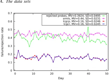
0 0.1 0.2 0.3 0.4 0.5 0.6 0.7 0 10 20 30 40 50 fail ur e/r eject ion rat e Day rejected probes, MV=0.3924, SD=0.0495 srmls, MV=0.44, SD=0.0231 lcgcp, MV=0.16, SD=0.0246 lcgcr, MV=0.16, SD=0.0245
Fig. 1. Failure and rejection rates; the mean and standard deviation are computed over the experiments
Different capabilities have to be tested; in the following, we consider three of them: probe srm-ls tests the listing ability from a CE to a SE, probe lcg-cr tests the read ability from a CE to a SE, and probe lcg-cp tests the write ability alike. Thus, each CE works as a probe station, launching probes to test the functionalities between itself and each SE. For the Biomed grid a whole set of testing transactions (as we mentioned before: 29512) were launched each day for each of the three probe classes. After near two months running, information for 51 validated days were collected. In other words, 51 fully observed SEs by CEs result matrices were accumulated for each probe. Figure 1 shows the statistical profile of the probe outcomes2. Failure rates of lcg-cp and lcg-crare almost identical (ranges from 10% to 25%), while
2Note that here and in fig. 5 and 7, only the points associated to each experiment are meaningful; the lines between the experiments are added only for readability purpose
failure of srm-ls is significantly higher (ranges from 40% to 50%).
The probes themselves are gLite jobs, run by a regular Biomed user. Some of them fail (rejection) in the sense that gLite is not able to complete the job, denoting that some job management services may be down or misconfigured (e.g. authentication, brokering etc.). The job entries in fig. 1 shows the ratio of unsuccessful probes over all launched probes in this sense. In the following, we consider only the accepted probes, i.e. those which run to completion, reporting success or failure; this approach amounts to consider that the data access capacities are independent from job management. This is a reasonable hypothesis in a gLite infrastructure because file transfers involved in job management use dedicated storage space independent from the one tested by our probes. Separate testing is good practice in general; in this specific case, the high rejection rate (average 40%) and the high failure rate would act as a massive noise on each other, and would make CP more difficult if we tried a global approach.
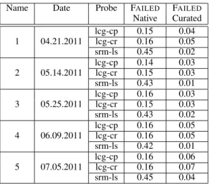
TABLE I FIVE EXAMPLE DATASETS
Name Date Probe FAILED FAILED
Native Curated lcg-cp 0.15 0.04 1 04.21.2011 lcg-cr 0.16 0.05 srm-ls 0.45 0.02 lcg-cp 0.14 0.03 2 05.14.2011 lcg-cr 0.15 0.03 srm-ls 0.43 0.01 lcg-cp 0.16 0.03 3 05.25.2011 lcg-cr 0.15 0.03 srm-ls 0.43 0.02 lcg-cp 0.16 0.05 4 06.09.2011 lcg-cr 0.16 0.05 srm-ls 0.42 0.01 lcg-cp 0.16 0.06 5 07.05.2011 lcg-cr 0.16 0.07 srm-ls 0.45 0.04
We selected five days for detailed performance analysis, refereed afterwards as the benchmarks. Table I shows some basic characteristics of the fully observed entries; the fourth column gives the failure rate when all probes are considered and exemplifies the need for inferring the structure of the apparently massive randomness. Figure 2 illustrates the struc-ture for lcg-cr and srm-ls on ’07-05-2011’, where the rows represent CEs and the columns stand for SEs. Each entry is the probe result between the corresponding CE and SE.
Black columns correspond to prolonged SE downtimes while black lines are CE failures leading to complete inability to communicate with any SE (e.g. network downtime or configuration issue). These are usually easily detected and reported by human operators with only a few incident reports. The scattered points correspond to local or transient issues, which are very difficult to handle due to the amount of incident reports independently generated. The higher failure rate of srm-ls compared to lcg-cr appears to be associated
10 20 30 40 50 60 70 80 90 100 20 40 60 80 100 120 140 160 SE CE 10 20 30 40 50 60 70 80 90 100 20 40 60 80 100 120 140 160 SE CE (a) lcg-cp (b) srm-ls
Fig. 2. The CE-SE matrix. Black =FAILED, white=OK
Fig. 3. Illustration of matrix recovery
with an inadequate port number in some probes, and may be considered as an example of a user error. Thus it could be argued that other, global (EGI-wide) monitoring tools should report on these systematic failures, and that the probe selection and prediction methods should be applied only to the more elusive causes of errors. While this is disputable (remember that all probes succeed as jobs, thus at least the CEs are up and running), it is worth assessing the performance of the methods when these systematic errors are eliminated. We thus designed a second set of experiments, with curated matrices as the reference fault structure. A curated matrix is a new original matrix, where the lines and columns with only failed entries (black ones in figure 2) have been removed prior to analysis. Their basic statistics are shown in the last column of table I. In this case, srm-ls shows a lower error rate than the other probes.
B. Evaluation Methodology
From this dataset, evaluating probe selection is straight-forward. Figure 3 illustrates the general workflow of the selection-prediction process. The Original matrix is the ground truth: a fully observed result matrix obtained from the all-to-all monitoring runs (section II-A). Value -1 stands for probe result OK (negative) and 1 means FAILED (positive). The Selected matrix is generated by deleting a proper proportion of entries in the Original one. In a real-world, probe selection-based, monitoring, the remaining entries would be the only actually
launched probes. The Predicted matrix is the recovery result generated by the prediction algorithm based on the known entries in Selected, where the X entries are now set to 1 or -1. In the real world scenario they would be delivered to users.
Contrary to the recommendation systems, where there is no ground truth (the users do not rate all products), the collection of data presented in section IV-A provides the true values. Thus, the classical performance indicators for binary classifi-cation can be measured. They describe the various facets of the discrepancy between the Original and the Predicted matrices. • Accuracy: the ratio of correctly predicted entries over the
total number of entries.
• Indicators associated with the risks (confusion matrix): sensitivity, the proportion of actual positives that are correctly predicted; specificity, the proportion of actual negatives that are correctly predicted; precision, the ratio of true positives over all predicted positives, and the MCC (Matthews Correlation Coefficient), a correlation coefficient between the observed and predicted binary classifications that is relatively insensitive to unbalanced positives and negatives.
• The AUC (Area Under ROC Curve), which summarizes the intrinsic quality of a binary classifier independent of the decision threshold.
The interest of MCC and AUC comes from the fact that, in the optimization step of MMMF, the classification error on the Selected matrix is a reasonable estimation of the prediction error, while this hypothesis is less natural for estimating MCC and AUC [16]. Thus, MCC and AUC provide a comparison indicator of the performance of the methods beyond their explicit optimization target.
In order to evaluate the contribution of the prediction (or coupled selection-prediction) methods, we compare their results with a simple baseline, called Rand Guess in the following. Rand Guess predicts entries following the distri-bution of the sample set (Selected matrix). For example if the ratio of positive:negative entries in a sample set is 1:4, then Rand Guess would predict an unknown entry as failed or positive with a probability of 20% and as ok or negative with a probability of 80%.
C. Static - Uniform
For each result matrix M different fractions of its entries are deleted uniformly and a series of partially observed matrices M10, M20, ... are generated. For these new matrices, the task is only to predict the deleted entries from the selected ones by MMMF-based CP. Figure 4 shows the prediction accuracy as a function of the fraction of launched probes, for the five benchmarks. The results are averages over ten experiments; as lcg-cp and lcd-cr behave similarly, only one is shown. The first and striking result is that an excellent performance can be reached with a tiny fraction of the original probes, typically 5%. The Rand Guess results are plotted for comparison pur-pose, but can be approximated easily: if q is the fraction of positive entries in the original matrix, then in the deleted part, P (True Positive) = P (Positive)P (Predicted Positive) = q2,
0.1 0.2 0.3 0.4 0.5 0.6 0.7 0.8 0.9 1 0.01 0.1 A cc uracy Probe fraction 04-21 static 05-14 static 05-25 static 06-09 static 07-05 static 04-21 random 05-14 random 05-25 random 06-09 random 07-05 random (a) lcg-cp 0.1 0.2 0.3 0.4 0.5 0.6 0.7 0.8 0.9 1 0.01 0.1 A cc uracy Probe fraction 04-21 static 05-14 static 05-25 static 06-09 static 07-05 static 04-21 random 05-14 random 05-25 random 06-09 random 07-05 random (b) srm-ls
Fig. 4. Accuracy for the Static-Uniform probe selection.
and similarly P (True Negative) = (1 − q)2; overall, the accuracy is q2+ (1 − q)2. With the values of q from table I, the accuracy of Rand Guess is in the order of 0.7 for lcg-cpand lcg-cr, and 0.5 for srm-ls.
20 40 60 80 100 120 0 10 20 30 40 50 R ank Day lcg-cp predicted lcg-cp real lcg-cr predicted lcg-cr real srm-ls predicted srm-ls real
Fig. 5. Rank comparison for the Static-Uniform probe selection
0.6 0.65 0.7 0.75 0.8 0.85 0.9 0.95 1 0 0.02 0.04 0.06 0.08 0.1 TPR : T ru e P osit ive R a te
FPR: False Positive Rate
static_lcgcp static_lcgcr static_srmls
Fig. 6. ROC values for the Static-Uniform probe selection. Note the range of the axes, which cover only the small part of the ROC space where the results belong, thus the diagonal line is not visible on the plot
0.86 0.88 0.9 0.92 0.94 0.96 0.98 1 10 20 30 40 50 AUC : Ar ea Under Cu rve Day lcgcp lcgcr srmls
Fig. 7. AUC for the Static-Uniform probe selection
responds to the hidden causes. Figure 5 shows the ranks of the predicted and original matrices. The ranks of the predicted matrices are significantly lower than the original ones, showing that a small number of causes dominates the overall behavior. The number of hidden causes is much larger for lcg-cp and lcg-crthan for srm-ls, confirming the empirical evidence that the srm-ls faults are more deterministic.
Figure 6 is the classical visualization of the confusion matrix in the ROC space for all the 51 days at 90% deletion rate (keeping 10% of the probes). Perfect prediction would yield a point in the upper left corner at coordinate (0,1) of the ROC space, representing 100% sensitivity (no false negatives) and 100% specificity (no false positives). The srm-ls dataset shows excellent prediction performance, being mostly very close to (0,1); lcg-cp and lcg-cr exhibit close ROC value distributions, definitely much better than a random guess, which lies on the diagonal line.
The other indicators also show excellent performance: the AUC (fig. 7) as well as the MCC are close to 1.
The problem becomes much more difficult when the
0.1 0.2 0.3 0.4 0.5 0.6 0.7 0.8 0.9 1 0.01 0.1 A cc uracy Probe fraction 04-21 05-14 05-25 06-09 07-05
Fig. 8. Accuracy for the Static-Uniform probe selection, curated srm-ls.
tematic faults are excluded, thus taking the curated matrices as inputs. Figure 8 shows the prediction accuracy on the curated srm-ls example (figures for the other probes are omitted for lack of space; note that, from table I, this probe is the most challenging one). As before, at most 10% of the whole probes is needed to reach a promising accuracy, greater than 98%. However, as the number of failed entries left in the curated matrices is much less than in the un-curated ones, e.g. the fraction of failed entries on srm-ls, 04-21-2011 drops from 45.37% to 2.25%, accuracy is not meaningful: predicting all entries as negative would give a similar result. The ability of making good prediction on the failed entries should be valued more. And the relevant performance indicators are not so good: for the same example, at 10% deletion rate, sensitivity is 0.41, meaning that 59% of the failures are not predicted, and precision is 0.49, meaning that amongst the predicted failures, 51% are spurious. The first strategy to tackle this issue is Active Probing.
D. Active Probing
In this experiment, we compare the Active Probing strategy with the Static one at equal probing cost: first, a Static-Uniform method is applied, in order to get the reference information, then more probes are selected with the min-margin heuristic for Active Probing, while for the Static-Uniform method, the same number of probes are selected uniformly at random.
Active Probing does improve accuracy (figure omitted). However, as explained in the previous section, the quality of failure prediction is the most important goal in this context. The comparison for the relevant indicators are detailed for the initial probe fraction equal to 5%, then adding probes by step of 5% fractions. The results as given for a total of 10% and 15% probes. Figure 9 shows sensitivity, precision and the MCC. The most important result is that Active Probing always outperforms Static-Uniform. In fact, the performance of the Static-Uniform strategy is bad, except for 07-05-2011 (day 5). The performance bears some relation with the failure rate of the benchmark (table I): larger failure rates in the
0 0.2 0.4 0.6 0.8 1 1 2 3 4 5 Sen sitivit y Benchmark number 0.05-mean tpr
0.1-mean tpr -S 0.15-mean tpr -S0.1-mean tpr -A 0.15-mean tpr -A
(a) Sensitivity 0 0.2 0.4 0.6 0.8 1 1 2 3 4 5 P recis ion Benchmark number 0.05-mean ppv
0.1-mean ppv -S 0.15-mean ppv -S0.1-mean ppv -A 0.15-mean ppv -A
(b) Precision 0 0.2 0.4 0.6 0.8 1 1 2 3 4 5 MC C: Mat thews cor rela tion co efficie nt Benchmark number 0.05-mean mcc 0.1-mean mcc -S 0.1-mean mcc -A 0.15-mean mcc -S 0.15-mean mcc -A (c) MCC
Fig. 9. Performance comparison for Static-uniform and Active Probing, curated srm-ls for the five benchmarks.
original curated matrix help uncovering the structure of the faults, even at quite low levels: with 4% failure rate, the 07-05-2011benchmark exhibits acceptable performance when keeping only 5% of the probes and the Static-Uniform strategy. However, the failure rate does not tell the full story: days 2 and 4 have the same low one (1%), but the performance on day 2 is much lower than on day 4. The likely explanation is that faults at day 2 do not present much correlation, while faults day 4 derive from a small number of shared causes.
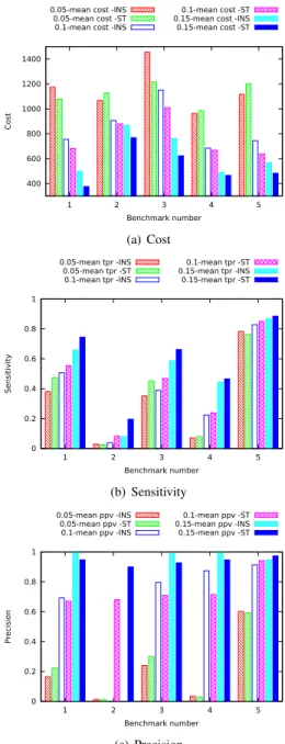
400 600 800 1000 1200 1400 1 2 3 4 5 Cost Benchmark number 0.05-mean cost -INS
0.05-mean cost -ST 0.1-mean cost -INS
0.1-mean cost -ST 0.15-mean cost -INS 0.15-mean cost -ST (a) Cost 0 0.2 0.4 0.6 0.8 1 1 2 3 4 5 Sen sitivit y Benchmark number 0.05-mean tpr -INS 0.05-mean tpr -ST 0.1-mean tpr -INS 0.1-mean tpr -ST 0.15-mean tpr -INS 0.15-mean tpr -ST (b) Sensitivity 0 0.2 0.4 0.6 0.8 1 1 2 3 4 5 P recis ion Benchmark number 0.05-mean ppv -INS 0.05-mean ppv -ST 0.1-mean ppv -INS 0.1-mean ppv -ST 0.15-mean ppv -INS 0.15-mean ppv -ST (c) Precision
Fig. 10. Cost and performance comparison between the Cost-Sensitive and Cost-Insensitive active probing, curated srm-ls for the five benchmarks.
E. Cost sensitive + Active probing
Finally, we sketch the results of the cost-sensitive MMMF. The C+/C− ratio is set equal to 10. The optimization target being soft-margin, the results for the initial Static-Uniform at 5% probe fraction are slightly different from the previous experiments. Figure 10 compares Active probing with and without cost weighting. Higher penalization of false negatives almost always decreases the final mis-prediction costs (Figure 10 (a)). Figure 10 (b) and (c) give the explanation: while sensitivity is indeed increased, the number of false positives also increases, leading to slightly lower precision, but the overall impact is favorable.
F. Computational cost
CP methods have to be scalable, as they target enormous dat set such as the Netflix database. The computational cost of the optimization problem of learning a MMMF essentially depends on the number of known entries in the Selected matrix, or equivalently on the probe fraction. Technically, the optimization is performed through a sparse dual semi-definite program (SDP), with the number of variables equal to the number of observed entries. We used YALMIP [17] as the model tool and CSDP [18] as the SDP solver. Empirically, the time needed for computing one MMMF increases expo-nentially with the number of entries in the Selected matrix. In practice, computation time is not an issue: less than 30 seconds with 2000 entries (15% probes) on a standard workstation.
V. RELATEDWORK
Collaborative Prediction associated with end-to-end prob-ing, with the components structure considered as a black box, participates in the general Quality of Experience approach [19]. More precisely, an important ingredient separating QoE from QoS is binary (possibly extended to discrete) clas-sification. Most work in this area is devoted to network-based services (e.g. among many others [20]). Before QoE became a popular keyword, Rish and Tesauro [13] explored the combination of MMMF and Active probing for the selection of good servers in various distributed and P2P systems. Our work combines the goal of proposing fault-free services to the user exemplified in [11], [21], and the CP approach of [13]. Z. Zheng and M.R. Lyu propose explicit users collaboration for estimating failure probabilities [21]; while their end-to-end framework is related to ours, the goal is more in line with QoS (estimating the full distribution of probability instead of binary classification), and the correlation amongst users or services is modeled by ad hoc methods. To our knowledge, this paper is the first one to exemplify MMMF on the fault prediction problem. In the limits of this paper, we cannot seriously discuss the merits of alternative strategies for CP. Amongst them, SVD++ [22], incorporates much a priori modeling related to the specifics of human rating. Bi-LDA [23] provides a quantified model of latent factors, which, like LDA, could be exploited for interpretation [24] more easily than MMMF.
VI. CONCLUSION
The Achille’s heel of large scale production grids and clouds is reliability. Quality of Experience at reasonable human cost requires extracting the hidden information from monitoring data whose intrusiveness should be limited. Collaborative Prediction is one of the promising and scalable strategies that can address this goal. This paper demonstrates its effectiveness on a large experimental dataset. Further work will consider two avenues: exploiting the resulting knowledge -the hidden causes uncovered by CP - towards diagnosis, as briefly sketched in section II-B; and improving prediction by separating transient failures from more permanent non-systematic ones, with tem-poral models inspired from the hierarchical Hidden Markov Models approach of text mining.
ACKNOWLEDGMENTS
This work has been partially supported by the European Infrastructure Project EGI-InsPIRE INFSO-RI-261323, by France-Grilles, and by the Chinese Scholarship Council.
REFERENCES
[1] H. Blodget. (2011, April) Amazon’s cloud crash disaster permanently destroyed many customers’ data. Business Insider. [Online]. Available: http://www.businessinsider.com/amazon-lost-data-2011-4
[2] N. Srebro, J. D. M. Rennie, and T. S. Jaakola, “Maximum-margin matrix factorization,” in Advances in Neural Information Processing Systems 17, 2005, pp. 1329–1336.
[3] E. Laure and al, “Programming the Grid with gLite,” pp. 33–45, 2006. [4] I. Foster, “The globus toolkit for grid computing,” in IEEE Int. Symp.
on Cluster Computing and the Grid, 2001.
[5] M. Ellert and al., “Advanced resource connector middleware for lightweight computational grids,” Future Generation Computer Systems, vol. 23, no. 2, pp. 219 – 240, 2007.
[6] A. Tsaregorodtsev and al., “DIRAC3 . The New Generation of the LHCb Grid Software,” Journal of Physics: Conference Series, vol. 219, no. 6, p. 062029, 2009.
[7] J. T. Moscicki, “Diane - distributed analysis environment for grid-enabled simulation and analysis of physics data,” in Nuclear Science Symposium Conference Record, 2003 IEEE, vol. 3, 2003, pp. 1617– 1620 Vol.3.
[8] S. Bagnasco and al., “Alien: Alice environment on the grid,” Journal of Physics: Conference Series, vol. 119, no. 6, p. 062012, 2008. [9] T. Maeno, “Panda: distributed production and distributed analysis system
for atlas,” Journal of Physics: Conference Series, vol. 119, no. 6, p. 062036, 2008.
[10] S. Andreozzi and al., “Glue Schema Specification, V.2.0,” http://www.ogf.org/documents/GFD.147.pdf, Tech. Rep., 2009. [11] I. Rish and al., “Adaptive diagnosis in distributed systems,” IEEE Trans.
Neural Networks, vol. 16, no. 5, pp. 1088 – 1109, 2005.
[12] S. Tong and D. Koller, “Support vector machine active learning with applications to text classification,” J. Mach. Learn. Res., vol. 2, March 2002.
[13] I. Rish and G. Tesauro, “Estimating end-to-end performance by col-laborative prediction with active sampling,” in Integrated Network Management, 2007, pp. 294–303.
[14] K. Morik, P. Brockhausen, and T. Joachims, “Combining statistical learning with a knowledge-based approach - a case study in intensive care monitoring,” in 16th Int. Conf. on Machine Learning, 1999, pp. 268–277.
[15] Y. Lin, G. Wahba, H. Zhang, and Y. Lee, “Statistical properties and adaptive tuning of support vector machines,” Machine Learning, vol. 48, pp. 115–136, September 2002.
[16] T. Joachims, “A support vector method for multivariate performance measures,” in International Conference on Machine Learning (ICML), 2005, pp. 377–384.
[17] J. Lfberg, “Yalmip : A toolbox for modeling and optimization in MAT-LAB,” 2004. [Online]. Available: http://users.isy.liu.se/johanl/yalmip [18] B. Borchers., “Csdp, a c library for semidefinite programming.”
Opti-mization Methods and Software, vol. 11(1), pp. 613–623, 1999. [19] H. Rifai, S. Mohammed, and A. Mellouk, “A brief synthesis of
QoS-QoE methodologies,” in 10th Int. Symp. on Programming and Systems, 2011, pp. 32–38.
[20] H. Tran and A. Mellouk, “Qoe model driven for network services,” in Wired/Wireless Internet Communications, ser. LNCS, 2010, vol. 6074, pp. 264–277.
[21] Z. Zheng and M. R. Lyu, “Collaborative reliability prediction of service-oriented systems,” in 32nd ACM/IEEE Int. Conf. on Software Engineer-ing, 2010.
[22] Y. Koren, “Factorization meets the neighborhood: a multifaceted collab-orative filtering model,” in 14th ACM SIGKDD int. conf. on Knowledge discovery and data mining, 2008, pp. 426–434.
[23] I. Porteous, E. Bart, and M. Welling, “Multi-hdp: a non parametric bayesian model for tensor factorization,” in 23rd Conf. on Artificial Intelligence, 2008, pp. 1487–1490.
[24] T. L. Griffiths and M. Steyvers, “Finding scientific topics,” Procs of the National Academy of Sciences, vol. 101, pp. 5228–5235, 2004.