Computing stationary distribution locally

Computing Stationary Distribution Locally

by

Christina Lee

B.S. in Computer Science, California Institute of Technology, 2011

Submitted to the Department of Electrical Engineering and Computer Science in partial fulfillment of the requirements for the degree of

ARCHNES

Master of Science

in Electrical Engineering and Computer Science at the Massachusetts Institute of Technology

June 2013

@ 2013 Massachusetts Institute of Technology All Rights Reserved.

2 i

Signature of Author:

Department of Electrical Engineering and

Christina Lee Computer Science May 22, 2013 Certified by:

Professor of Electrical Engineeri

Certified by:

clX

Professor of Electrical Engineeri

f

Asuman Ozaglar ng and Computer Science Thesis Supervisor

Devavrat Shah ng and Computer Science Thesis Supervisor Accepted by:

/

/

(&eslie A. Kolodziejski Professor of Electrical Engineering and Computer Science Chair, Committee for Graduate Students

Computing Stationary Distribution Locally

by Christina Lee

Submitted to the Department of Electrical Engineering and Computer Science in partial fulfillment of the requirements for the degree of

Master of Science Abstract

Computing stationary probabilities of states in a large countable state space Markov Chain (MC) has become central to many modern scientific disciplines, whether in statis-tical inference problems, or in network analyses. Standard methods involve large matrix multiplications as in power iterations, or long simulations of random walks to sample states from the stationary distribution, as in Markov Chain Monte Carlo (MCMC). However, these approaches lack clear guarantees for convergence rates in the general setting. When the state space is prohibitively large, even algorithms that scale linearly in the size of the state space and require computation on behalf of every node in the state space are too expensive.

In this thesis, we set out to address this outstanding challenge of computing the stationary probability of a given state in a Markov chain locally, efficiently, and with provable performance guarantees. We provide a novel algorithm, that answers whether a given state has stationary probability smaller or larger than a given value A

E

(0, 1). Our algorithm accesses only a local neighborhood of the given state of interest, with respect to the graph induced between states of the Markov chain through its transi-tions. The algorithm can be viewed as a truncated Monte Carlo method. We provide correctness and convergence rate guarantees for this method that highlight the depen-dence on the truncation threshold and the mixing properties of the graph. Simulation results complementing our theoretical guarantees suggest that this method is effective when our interest is in finding states with high stationary probability.

Thesis Supervisor: Asuman Ozdaglar

Title: Professor of Electrical Engineering and Computer Science Thesis Supervisor: Devavrat Shah

Title: Professor of Electrical Engineering and Computer Science

Acknowledgments

This thesis owes its existence to Professor Devavrat Shah and Professor Asuman Ozdaglar. It has been an incredible joy to work with them both, and I could tell stories upon stories of the encouragement and inspiration they have been to me. They have been incredibly patient with me and always put my personal growth as a researcher first. I have learned so much from them about how to approach the process of learning and research, and how to face those moments when progress seems so slow. I remember countless meetings in which I walked in frustrated, yet walked out encouraged and excited again. I appre-ciate Devavrat's inspirational analogies, reminding me that grad school is a marathon, not a sprint. I'd like to thank Asu for her warm support and patience in teaching me how to communicate clearly and effectively.

I am also incredibly grateful to the LIDS community. Truly the spirit of the LIDS community matches the bright colors of the LIDS lounge, always able to put a smile on my face. A special thanks goes to my great officemates Ammar, Iman, Yuan, Katie, and Luis for sharing both in my excited moments as well as my frustrated moments. I appreciate their encouragement and reminders to take a break and relax when I am too stuck. I am grateful for Ermin, Annie, Kimon, Elie, Ozan, and Jenny as well for bouncing ideas with me and encouraging me along in my research as well. I am in debt to the amazing community of LIDS girls: Shen Shen, Henghui, Mitra, and Noele, who

have colored my days and made my time here full of laughter.

A big thanks to the Graduate Christian Fellowship at MIT and the Park Street Church International Fellowship, which have become my family in Boston. As always, I am forever grateful to my parents unending support and my siblings encourgement. Finally, the biggest thanks goes to my greatest supporter: to God who reminds me every day that I am his beloved child. His love frees me from unhealthy pressures and fills me with joy and strength each day.

Contents

Abstract 3 Acknowledgments 4 List of Figures 9 1 Introduction 11 1.1 M otivation . . . . 11 1.2 Related Literature . . . . 14 1.3 Contributions . . . . 20 1.4 O utline . . . . 21 2 Preliminaries 23 2.1 M arkov chains . . . . 23 2.2 Foster-Lyapunov analysis . . . . 27

2.3 Concentration of random variables . . . . 29

2.4 Monte Carlo Methods for Pagerank . . . . 30

3 Algorithm 35 3.1 Problem Statement . . . . 35

3.2 Monte Carlo Return Time (MCRT) Algorithm . . . . 37

3.3 Bias correction . . . . 40

4 Theoretical Guarantees 41 4.1 M ain Theorem . . . . 41

4.2 Finite State Space Markov Chain . . . . 47

4.3 Countable-state space Markov Chain . . . . 55

5 Estimating Multiple Nodes Simultaneously 63 5.1 Multiple Node (MCRT-Multi) Algorithm . . . . 63

5.2 Theoretical Analysis . . . . 65

8 CONTENTS

6 Examples and Simulations 69

6.1 Queueing System ... . 69

6.2 PageRank ... ... 75 6.3 Magnet Graph ... ... 84

7 Conclusion 87

List of Figures

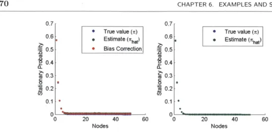
3.1 Graph of a clique plus loop . . . . 35 4.1 Lyapunov decomposition of SS . . . . 56 6.1 M M 1 Q ueue. . . . .. . . . ... 69 6.2 MM1 Queue (left) Estimates from the MCRT algorithm, (right)

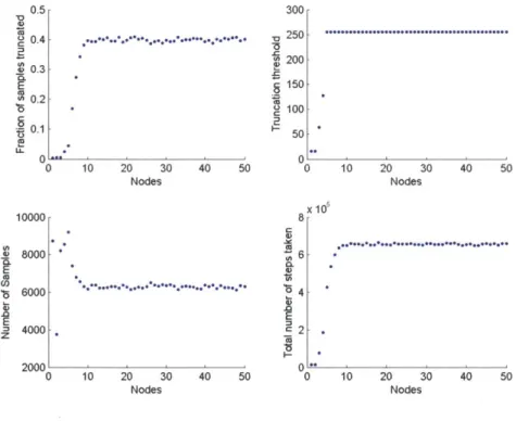
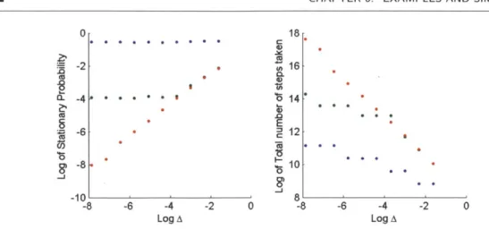
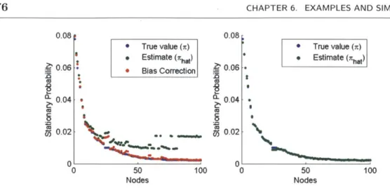
Esti-mates from the MCRT-Multi algorithm. . . . . 70 6.3 MM1 Queue -Statistics from the MCRT algorithm . . . . 71 6.4 MM1 Queue -Results of the MCRT algorithm as a function of A . . . 72 6.5 MM1 -Convergence rate analysis . . . . 75 6.6 PageRank -(left) Estimates from the MCRT algorithm, (right)

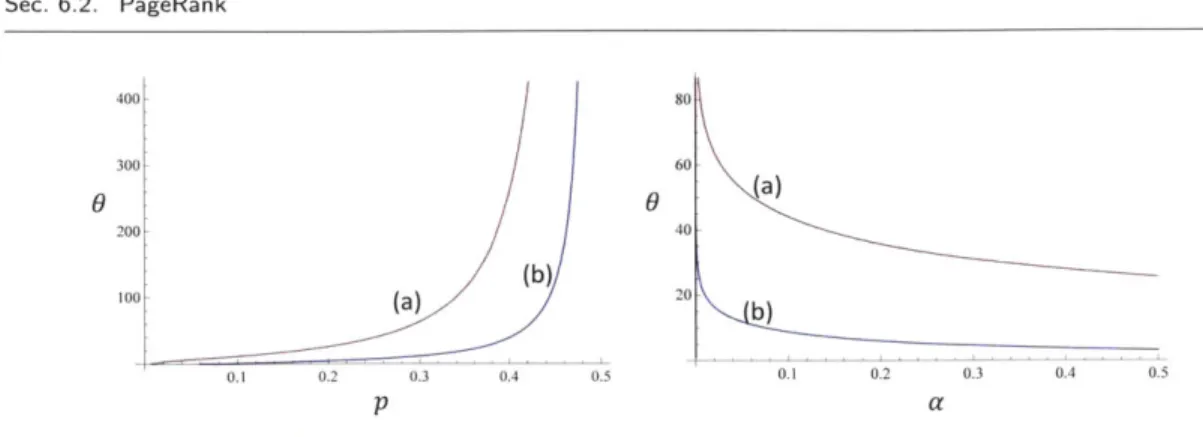
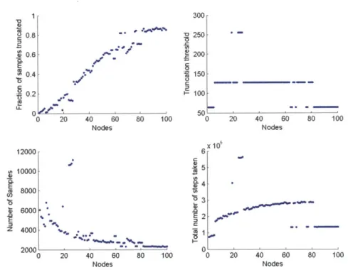
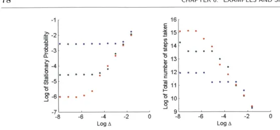
Esti-mates from the MCRT-Multi algorithm. . . . . 76 6.7 PageRank -Statistics from the MCRT algorithm. . . . . 77 6.8 PageRank -Results of the MCRT algorithm as a function of A . . . . . 78 6.9 PageRank -Results of the MCRT algorithm as a function of

#

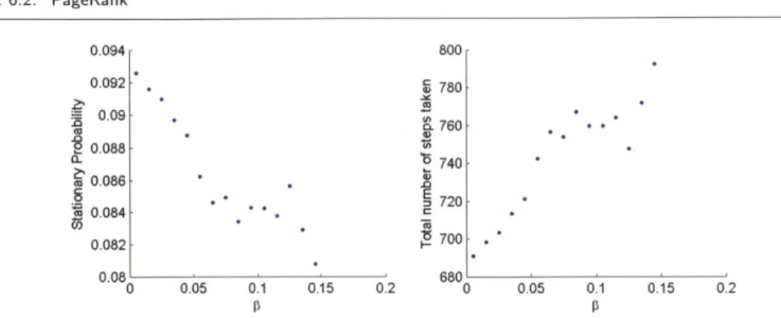
for a high

degree node . . . . 83 6.10 PageRank -Results of the MCRT algorithm as a function of 0 for a low

degree node ... ... 83 6.11 M agnet M arkov chain. . . . . 84 6.12 Magnet -(left) plots the results of the MCRT algorithm, (right) plots

the results of the MCRT-Multi algorithm. . . . . 85 6.13 Magnet -Statistics from the MCRT algorithm. . . . . 86

Chapter 1

Introduction

U 1.1 Motivation

The computation of the stationary distribution of a Markov chain (MC) with a very large state space (large finite, or countably infinite) has become central to many

sta-tistical inference problems. The Markov Chain Monte Carlo (MCMC) coupled with

Metropolis Hasting's rule or Gibbs sampling is commonly used in such computations. The ability to tractably simulate MCs along with the generic applicability has made the MCMC a method of choice and arguably the top algorithm of the twentieth century.1 However, MCMC (and its variations) suffer from a few limitations especially for MCs with very large state space. The MCMC methods involve sampling states from a long random walk over the entire state space [18, 25]. The random walks need to be "long enough" to produce reasonable approximations for the stationary distribution, yet it is difficult to analyze and establish theoretical guarantees for the convergence rates. Furthermore, a large enough number of samples must be used in order to ensure that the distribution has been fully sampled from.

Stationary distributions of Markov chains are also central to network analysis. Net-works have become ubiquitous representations for capturing interactions and relation-ships between entities across many disciplines, including social interactions between

'The Top Ten Algorithms of the Century.

http://orion.math.iastate.edu/burkardt/misc/algorithms-dongarra.html

12 CHAPTER 1. INTRODUCTION

individuals, interdependence between financial institutions, hyper-link structure be-tween web-pages, or correlations bebe-tween distinct events. Many decision problems over networks rely on information about the importance of different nodes as quantified by network centrality measures. Network centrality measures are functions assigning "im-portance" values to each node in the network. The stationary distribution of specific random walks on these underlying networks are used as network centrality measures in many settings. A few examples include PageRank: which is commonly used in Internet search algorithms [29], the Bonacich centrality and eigencentrality measures: encoun-tered in the analysis of social networks [9, 10, 28], rumor centrality: utilized for finding influential individuals in social media like Twitter [32], and rank centrality: used to find a ranking over items within a network of pairwise comparisons [27].

The power-iteration method is currently the method commonly used for computing stationary disributions of random walks over networks, such as PageRank. The method involves iterative multiplication of the transition probability matrix of the random walk [16]. Again, this method suffers from similar limitations for large networks: there is no clearly defined stopping condition or convergence analysis for general settings, and it requires computation from every node in the network. While this can be implemented in a distributed manner using a message passing algorithm (which involves computations that use information from neighbors of a node), convergence rates are often hard to establish.

The massive size of the state space of these Markov chains is the primary reason for development of super-computation capabilities - be it nuclear physics [24, Chapter 8], Google's computation of PageRank [29] or Stochastic simulation at-large [3]. In the presence of Markov chains with massive state space, an ideal algorithm would be the one that overcomes both of these limitations. In this thesis, motivated by this goal, we present a local algorithm to approximate the stationary probability of a

Sec. 1.1. Motivation 13 node exploiting only local information in a subnetwork around that node. By local, we mean two things. First, the algorithm must be easily distributed. The algorithm must only access the network through neighbor queries, and computation at a node can only use local information passed through his neighbors. Second, the algorithm must be "local" to the nodes of interest. For example, if we are only interested in computing the stationary probability of a single node, then all computation involved in the algorithm must be restricted to this node, where computation refers to any arithmetic operations or operations involving memory. There are many benefits for having such a local algorithm.

First, in many settings such as ranking, we are not actually interested in computing the stationary probabilities of all nodes. In web search or movie and restaurant recom-mendation settings, only the scoring among top nodes are relevant, since users often only view the first page of results. Rather than computing the entire stationary distri-bution, we may only need to compute the stationary probabilities of a smaller specific subset of nodes. Thus we desire algorithm that scales with the size of this subset rather than with the full size of the network.

Second, there may be physical constraints for accessing or storing the information that prohibit global computation. For example, the information may be stored in a distributed manner either due to memory limitations or the nature of the data. In citation networks, the information is inherently not centralized (i.e. not owned by a single central agent). It may be easy to query a single paper or a single author to view the neighborhood of that node, however performing any global computation would require first crawling through searching node by node to rebuild the network. Many search engines maintain indexes containing the entire webgraph, yet due to the sheer size of the web, the information must be distributed among clusters of computers. Some estimate that the size of the web is growing at a rate of 21% new webpages every year.2

2

14 CHAPTER 1. INTRODUCTION

This causes increasing difficulty for methods such as power iteration, which require computation at every node in the network.

Third, there may be privacy constraints that prevent an external agent from access-ing the global network. For example, in many online social networks, privacy settaccess-ings only allow a member to access his local network within a small distance (e.g. friends of friends). There exist APIs that allow external companies to interface with Facebook's social network data. However, every user must specifically grant the company access to his or her local network. Companies offer users the ability to use new applications or play new games in exchange for the access rights to their social network. Companies design their applications and games to have a social aspect so that after a user adopts a new appliation, he will have incentives for his friends to also join this application. Thus, many of these applications and games are adopted through viral behavior, by friends recommending them to their friends. Thus, a company will often gain access rights to clusters or local snapshots of the network. A local algorithm that only requires information from a neighborhood around a specific node can still provide estimates for global properties such as stationary distribution, using the limited information from these clusters.

N

1.2 Related Literature

In this section, we provide a brief overview of the standard methods used for computing stationary distributions. Computation of the stationary distribution of a MC is widely applicable with MCMC being utilized across a variety of domains. Therefore, the related prior work is very large. We have chosen few samples from the literature that we think are the most relevant.

Monte Carlo Markov Chain. MCMC was originally proposed in [25], and a tractable

Sec. 1.2. Related Literature 15 way to design a random walk for a target stationary distribution was proposed by Hastings [18]. Given a distribution 7r(x), the method designs a Markov chain such that the stationary distribution of the Markov chain is equal to the target distribution. Without formally using the full transition matrix of the designed Markov chain, Monte Carlo sampling techniques can be used to estimate this distribution by sampling random walks via the transition probabilities at each node.

Each transition step in the Markov chain is computed by first sampling a transition from an "easy" irreducible Markov chain. Assume the state space is represented by an n-length 0-1 vector in

{0,

1}f. A commonly used "easy" Markov chain is such that from a node x, a transition to x' is computed by randomly selecting a coordinate

i E 1, 2, ... n and flipping the value of x at that coordinate. Then this transition is accepted or rejected with probability min

(I

,1).

The stationary distribution of this Markov chain is equal to 7r. After the length of this random walk exceeds the mixing time, then the distribution over the current state of the random walk will be a close approximation for the stationary distribution. Thus the observed current state of the random walk is used as an approximate sample from 7r. This process is repeated many times to collect independent samples from ri.

Overview articles by Diaconis and Saloff-Coste

[13]

and Diaconis [12] provide a summary of the major development from probability theory perspective. The majority of work following the initial introduction of the algorithm involves trying to gain un-derstanding and theoretical guarantees for the convergence rates of this random walk. Developments in analyzing mixing times of Markov chains are summarized in books by Aldous and Fill [1] and Levin, Peres and Wilmer [23]. The majority of results are limited to reversible Markov chains, which are equivalent to random walks on weighted undirected graphs. Typical techniques analyzing convergence rates involve spectral analysis or coupling arguments. Graph properties such as conductance provide ways to

16 CHAPTER 1. INTRODUCTION

characterize the spectrum of the graph. In general, this is a hard open problem, and there are few practical problems that have precise convergence rate bounds, especially when the Markov chain may not be reversible.

Power Iteration. The power-iteration method (cf. [16,22,33]) is an equally old and well-established method for computing leading eigenvectors of matrices. Given a ma-trix A and a seed vector x0, recursively compute iterates xt+1 = _IlAxtiL Axt If matrix A_Ifmti* has a single unique eigenvalue that is strictly greater in magnitude than other eigen-values, and if x0 is not orthogonal to the eigenvector associated with the dominant eigenvalue, then a subsequence of xt converges to the eigenvector associated with the dominant eigenvalue. This is the basic method used by Google to compute PageRank. Recursive multiplications involving large matrices can become expensive very fast as the matrix grows. When the matrix is sparse, computation can be saved by implementing it through 'message-passing' techniques; however it still requires computation to occur at every node in the state space. The convergence rate is governed by the spectral gap, or the ratio between the two largest eigenvalues. Techniques used for analyzing mixing times for MCMC methods as discussed above are also useful for understanding the convergence of power iteration. For example, for reversible Markov chains, the con-ductance of the graph is directly related to the spectral gap. For large MCs, the mixing properties may scale poorly with the size, making it difficult to obtain good estimates in a reasonable amount of time.

In the setting of computing PageRank, there have been efforts to modify the algo-rithm to execute power iteration over subsets of the graph and combining the results to obtain global estimates. Kamvar et. al. observed that there may be obvious ways to partition the web graph (i.e. by domain names) such that power iteration can be used to estimate the local pagerank within these partitions [21]. They estimate the relative weights of these partitions, and combine the local pageranks within each

Sec. 1.2. Related Literature ₁₇

partition according to the weights to obtain a initial starting vector for the standard PageRank computation. Using this starting vector may improve the convergence rate of power iteration. Chen et. al. propose a method for estimating the PageRank of a subset of nodes given a local neighborhood

[11].

Their method uses heuristics such as weighted in-degree as estimates for the PageRank values of nodes on the boundary of the given neighborhood. After fixing the boundary estimates, standard power iteration is used to obtain estimates for nodes within the local neighborhood. The error in this method depends on how close the true pagerank of nodes on the boundary correspond to the heuristic guesses such as weighted in-degree.

Computing PageRank Locally. There has been much recent effort to develop local algorithms for computing properties of graphs [8], including PageRank. Given a directed network of n nodes with an n x n adjacency matrix A (i.e., Aj = 1 if (i, j) E E and 0 otherwise), the PageRank vector

7r

is given by the stationary distribution of a Markov chain over n states, whose transition matrix P is given by

P = (1 - /3)D- 1A + /1 .rT. (1.1)

Here D is a diagonal matrix whose diagonal entries are the out degrees of the nodes, 3 _{e (0, 1) is a fixed scalar, and r is a fixed probability vector over the n nodes.}3

Hence, in each step the random walk with probability (1 - 3) chooses one of the neighbors of the current node equally likely, and with probability

3

chooses any of the nodes in the network according to r. Thus, the PageRank vector 7r satisfies

7r T = 7rTP = (1- 0)7T D-1A +

#rT

(1.2)

where 7rT . 1 = _{1. This definition of PageRank is also known as personalized PageRank,}

18 CHAPTER 1. INTRODUCTION

because r can be tailored to the personal preferences of a particular web surfer. When

Ir = -1 .then 7r equals the standard global PageRank vector. If r = ei, then 7r describes the personalized PageRank that jumps back to node i with probability

#

in every step. Computationally, the design of local algorithms for personalized PageRank has been of interest since its discovery. However, only recently has rigorous analytic progress been made to establish performance guarantees for both known and novel algorithms. These results crucially rely on the specific structure of the random walk describing PageRank: P decomposes into a natural random walk matrix D- 1A, and a rank-1

matrix 1 - rT, with strictly positive weights (1 - 0) and

#

respectively, cf. (1.1). This structure of P has two key implications. Jeh and Widom [20] and Haveliwala [19] observed a key linearity relation - the global PageRank vector is the average of the n personalized PageRank vectors corresponding to those obtained by setting r = ei for 1 < i < n. That is, these n personalized PageRank vectors centered at each node

form a basis for all personalized PageRank vectors, including the global PageRank. Therefore, the problem boils down to computing the personalized PageRank for a given node. Forgaras et al. [14] used the fact that for the personalized PageRank centered

at a given node i (i.e., r = ei), the associated random walk has probability

#

at every step to jump back to node i. This is a renewal time for the random walk and hence by the standard renewal theory, the estimate of a node's stationary probability (or personalized PageRank) can be obtained through enough samples of renewal cycles along with standard concentration results.

Subsequent to the above two key observations, Avrachenkov et al. [4] surveyed variants to Fogaras' random walk algorithm, such as computing the frequency of visits to nodes across the complete sample path rather than only the end node. Bahmani

et al. [5] addressed how to incrementally update the PageRank vector for dynamically

Sec. 1.2. Related Literature 19

al. extended the algorithm to streaming graph models [30], and distributed computing

models [31], "stitching" together short random walks to obtain longer samples, and thus reducing communication overhead. More recently, building on the same sets of observation, Borgs et al. [7] provided a sublinear time algorithm for estimating global PageRank using multi-scale matrix sampling. They use geometric-length random walk samples, but do not need to sample for all n personalized PageRank vectors. The algorithm returns a set of "important" nodes such that the set contains all nodes with PageRank greater than a given threshold, A, and does not contain any node with PageRank less than A/c with probability 1 - o(1), for a given c > 3. The algorithm runs in time 0 (-polylog(n)).

Andersen et al. designed a backward variant of these algorithms [2]. Previously, to compute the global pagerank of a specific node

j,

we would average over all personalized pagerank vectors. The algorithm proposed by Andersen et al. estimates the global pagerank of a node

j

by approximating the "contribution vector", i.e. estimating for the jth coordinates of the personalized pagerank vectors that contribute the most to

7ry.

These algorithms are effectively local: to compute the personalized PageRank of a node i (i.e., r = ei), the sampled nodes are within distance distributed according to a geometric random variable with parameter 3, which is on average 1/3. The global PageRank computation requires personalized computation of other nodes as well but they can be performed asynchronously, in parallel. They allow for incremental updates as the network changes dynamically. However, all of these rely on the crucial property that the random walk has renewal time that is distributed geometrically with parameter 3 > 0 (that does not scale with network size n, like 1/n, for example). This is because the transition matrix P decomposes as per (1.1) with

/

E (0, 1), not scaling (down) with n. In general, the transition matrix of any irreducible, aperiodic, positive-recurrent Markov chain will not have such a decomposition property (and hence known renewal

time), making the above algorithms inapplicable.

* 1.3 Contributions

This thesis designs a local algorithm for estimating stationary distributions of general Markov chains. We develop a truncated Monte Carlo method, which answers the follow-ing question: for a given node i of a MC with a finite or countably infinite state-space, is the stationary probability of i larger or smaller than A, for a given threshold A

c

(0, 1)? Our proposed randomized algorithm utilizes only the 'local' neighborhood of the node i, where neighborhood is defined with respect to the transition graph of the Markov chain, to produce an approximate answer to this question. The algorithm's computation (as well as 'radius' of local neighborhood) scales inversely proportional to A. The algorithm has an easy to verify stopping condition with provable performance guarantees. For nodes such that

7ri

> A, we show in Theorem 4.2.1 that our estimate is within an eZmax multiplicative factor of the true 7ri, where Zmax is a function of the mixing properties of the graph. For nodes such that 7ri < A, we obtain an upper bound to label them as low probability nodes. Examples in Chapter 3 and Section 6.3 illustrate that any local algorithm cannot avoid the possibility of overestimating the stationary probabilities of nodes in settings where the graph mixes poorly.

The algorithm proposed is based on a basic property: the stationary probability of a node in a MC is the inverse of the average value of its "return time" under the MC. Therefore, one way to obtain a good estimate of stationary probability of a node is to sample return times to the node in the MC and use its empirical average to produce an estimate. To keep the algorithm "local", since return times can be arbitrary long, we truncated the sample return times at some threshold 0. In that sense, our algorithm is a truncated Monte Carlo method.

The optimal choice for the truncation parameter, the number of samples, and the

Sec. 1.4. Outline 21

stopping conditions is far from obvious when one wishes (a) to not utilize any prior information about MC for generic applicability, and (b) to provide provable performance guarantees. The key contribution of this paper lies in resolving this challenge by means of simple rules.

In establishing correctness and convergence properties of the algorithm, we utilize the exponential concentration of return times in Markov chains. For finite state Markov chains, such a result follows from known results (see Aldous and Fill [1]). For countably infinite state space Markov chains, we build upon a result by Hajek [17] on the con-centration of certain types of hitting times in order to prove that the return times to a node concentrate around its mean. We use these concentration results to upper bound the estimation error and the algorithm running time as a function of the truncation threshold 0 and the mixing properties of the graph. For graphs that mix quickly, the distribution over return times concentrates more sharply around its mean, and therefore we obtain tighter performance guarantees.

N

1.4 Outline

In Chapter 2, we give a brief overview of the fundamentals in Markov chains and probability theory needed to understand our results. In Chapter 3, we present the problem statement and our algorithm. In Chapter 4, we prove theoretical guarantees in both the finite state space and countably infinite state space settings. We show that the algorithm terminates in finite time, and with high probability, the estimate is an upper bound of the true value. Given specific properties of the Markov chain, we prove tighter concentration results for the tightness of our approximation as well as tighter bounds for the total running time. The tightness of our approximation will be limited by the mixing properties of the Markov chain. In Chapter 5, we propose an extension to the algorithm that allows us to reuse computation to estimate the stationary probabilities

22 CHAPTER 1. INTRODUCTION

of multiple nodes simultaneously. We similarly show guarantees for the tightness of our approximation as a function of the mixing properties of the Markov chain. In Chapter 6, we show simulation results of running our algorithm on specific MCs, verifying that the algorithm performs well in reasonable settings. We also show an example of a Markov chain that mixes poorly and discuss the limitations of our algorithm in that setting. Finally, we present closing remarks and discussion in Chapter 7.

Chapter 2

Preliminaries

* 2.1 Markov chains

For this thesis, we consider discrete-time, time-homogenous, countable state space Markov chains. A Markov chain with state space E and transition probability ma-trix P is a sequence of random variables

{Xt}

for t E

{0}

U Z+ such that

* For all t, Xt E E.

" P : E x E -- _{[0,1], and P is stochastic: For all i E E,}

1: Pig =1.

jE E

" {Xt} satisfies the Markov property:

P(Xt+1 = jnX = X0, X1 = X1.... Xt = = P(Xt+1 =

jXt

= = Pi.

Let P") denote the value of coordinate (x, y) of the matrix P'.

Definition 2.1.1. The Markov chain is irreducible if for all x,y E Z, there exists a, b E Z+ such that

p(a) > Jjy >0

0

and ad p(b) > xy 0.

24 CHAPTER 2. PRELIMINARIES

Definition 2.1.2. The Markov chain is aperiodic if for all x E E, there exists no G Z+

such that for all n > no,

p4n) > 0.

The Markov chain can be visualized as a random walk over a weighted directed graph G = (E, E), where E is the set of nodes, E {(i, j) E E x E : P > 0} is the

set of edges, and P describes the weights of the edges. We refer to G as the Markov

chain graph. The state space E is assumed to be either finite or countably infinite. If it

is finite, let n =

|El

denote the number of nodes in the network.1 If the Markov chain is irreducible, it is equivalent to the graph being strongly connected (for all x, y C E there exists a path from x to y). If the Markov chain is aperiodic, it is equivalent to the statement that the graph cannot be partitioned into more than one partition such that there are no edges within each partition (for example, a bipartite graph is not aperiodic). The local neighborhood of node i E E within distance r > 1 is defined as

{j E E : dG(i,j) < r}, where dG(i,j) is the length of the shortest directed path from i

to

j

in G.

Throughout the paper, we will use the notation E If({Xt})] = E[f({X})|Xo =i and Eu[f({Xt})] to denote the expectation of f({Xt}) under the condition that Xo is distributed uniformly over state space E (of course this is only well defined for a finite state space Markov chain). Similarly, we denote Pi(event) = P(event|Xo = i). Let the return time to a node i be defined as

Ti = inf{t > 11 Xt = i}, (2.1)

Throughout the paper, Markov chain and random walk on a network are used interchangeably; similarly nodes and states are used interchangeably. The stationary probability of a node quantifies the

Sec. 2.1. Markov chains 25 and let the maximal hitting time to a node i be defined as

Hi = max Ej [Ti]. (2.2)

jCE

The maximal hitting time may only be defined for finite state space Markov chains.

Definition 2.1.3. A Markov chain is recurrent if for all i C E,

Pi(T < OC) = 1.

Definition 2.1.4. A Markov chain is positive recurrent if for all i

e

E,

E [T] < oC.

We restrict ourselves to positive recurrent Markov chains. Since the expected return time is finite for all nodes, this means that the random walk cannot "drift to infinity". All irreducible finite Markov chains are positive recurrent, thus this property is only interesting in the countably infinite state space setting.

Definition 2.1.5. A function 7c : E -+ [0, 1] is a stationary distribution for the Markov

chain if

" For all i C

E,

7ei =E r jPji.

"

Eiez7ri=1.

In other words, if

7

describes a distribution over the state space, then after an ar-bitrary number of transitions in the Markov chain, the distribution remains the same.

rTpn = 7rT for all n. If the Markov chain is irreducible and positive recurrent, then

there exists a unique stationary distribution. Positive recurrence is equivalent to "sta-bility", and the stationary distribution captures the equilibrium of the system.

26 CHAPTER 2. PRELIMINARIES

It is well known [1, 26] that for any nodes i,

j

E E,

1

(2.3)

and

Ej[visits to node

j

before time T]

Ej [T] (2.4)

The fundamental matrix Z of a finite state space Markov chain is defined as

Z = (P(t)

t=o

i.e., the entries of the fundamental matrix Z are defined by

00

Zij = E(P. t=0

Entry Zij corresponds to how quickly a random walk beginning at node i mixes to node j. We restate here a few properties shown in Aldous and Fill [1] which will be useful

for our analysis.

Lemma 2.1.6. For i

j

zJj - Zj

Ili3

Lemma 2.1.7. For distinct i, k E, the expected number of visits to a node

j

beginning from node k before time T is equal to

Ek

[(

1

fxt=j11t

T1

=,r}(Ek[Ti] + E [Tj] - Ek[TJ]). t=1 . 26 CHAPTER 2. PRELIMINARIES 7r - = - 17r T) = (I_ -p + 17rT)~-1 - _7ri .

Sec. 2.2. Foster-Lyapunov analysis 27 E 2.2 Foster-Lyapunov analysis

Foster introduced a set of techniques for analyzing countable state space Markov chains. [15]

Theorem 2.2.1. Let

{X

1

}

be a discrete time, irreducible, aperiodic Markov chain on countable state space E with transition probability matrix P.

{Xt}

is positive recurrent if and only if there exists a Lyapunov function V : E - R+, '> 0 and b > 0, such that

1. For all x E

E,

E [V(Xt+1)|Xt = x] < oo,

2. For all x E E such that V(x) > b,

E [V(Xt+1 ) - V(Xt)|Xt = x] < -<.

In words, given a positive recurrent Markov chain, there exists a Lyapunov function

V : E -+ R+ and a decomposition of the state space into B =

{x

e E : V(x) < b} and

BC = {x E E : V(x) > b} such that there is a uniform negative drift in BC towards B and |BI is finite.

In fact, for any irreducible, aperiodic, Markov chain, the following function is a valid Lyapunov function. Choose any i E E.

V(x) = E[Tj|Xo = x]

where T = inf{t > 0 : Xt = i}. Thus B {i}. And V(i) = 0. For all x C E \ {i},

V(x) = 1+ Y PryV(y). YEE

28 CHAPTER 2. PRELIMINARIES

And thus,

PXyV(y) - V(x) = -1.

yEE

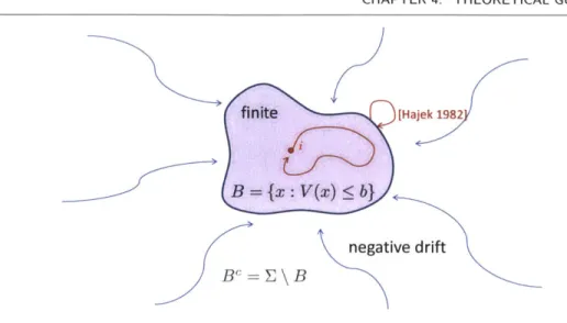
A Lyapunov function for a positive recurrent Markov chain helps to impose a natu-ral ordering over the state space that allows us to prove properties of the Markov chain. There have been many results following the introduction of the Foster-Lyapunov Cri-teria, which give bounds on the stationary probabilities, return times, and distribution of return times as a function of the Lyapunov function [6,17]. We present a result from Hajek that will be useful in our analysis.

Theorem 2.2.2 (Hajek 1982). [17] Let {Xt} be an irreducible, aperiodic, positive

re-current Markov chain on a countable state space E with transition probability matrix P. Assume that there exists a Lyapunov function V : E - R+ and values vmax,

Y

> 0,

and b > 0 such that

1. The set B = {x E _{E : V(x) < b} is finite,}

2. For all x, y c E such that P(Xt+1 =

jIXt

= i) > 0,

|V(j) - V (ij ) vmax,

3. For all x E E such that V(x) > b,

E [V(Xt+1) - V(Xt)|Xt = x] < -y.

Let the random variable TB = inf{t : Xt G B}. Then for any x such that V(x) > b, and

for any choice of constants w > 0, rl, p, and A satisfying

0< r min m ewmax 2

(ewvmax - (1 + Wvmax)) 2

p=1-7I + W2

1 0 < A < ln( ),

the following two inequalities hold:

P['TB _{> k|Xo = x] < ei(V(x) -b)Pk}

E[eATB|Xo = x] < en(V(x)-b) e 1.

1I - peA A concrete set of constants that satisfy the conditions above are

W =

1

- _ _ and p = 1 - . (2.5)

Vmax 2(e - 2)Vmlax' 4(e - 2)vltax

U 2.3 Concentration of random variables

In this section, we state fundamental theorems for the concentration of a sum of i.i.d. random variables.

Theorem 2.3.1 (Chernoff's Multiplicative Bound for Binomials).

Let {X 1, X2, X3,.. .XN} be a sequence of independent identically distributed Bernoulli

random variables, such that for all i, Xi = 1 with probability p and Xi = 0 otherwise. Then for any e > 0,

I N < Np _e Np

P N Xi- E[X] > CE[X] < +

< 2e- .

Theorem 2.3.2 (Chernoff's Multiplicative Bound for Bounded Variables).

Let {X 1, X2, X3,.... XN} be a sequence of independent identically distributed strictly

bounded random variables, such that Xi - X for all i, and X

e

[0, 0]. Then for any

29

30 CHAPTER 2. PRELIMINARIES e > 0, N)NE[X NE[X] P N X'1 - E[X] ;> EE[1X] 5 (+1+ + ,2NE[X] <2e- 3

E

2.4 Monte Carlo Methods for Pagerank

In this section, we present the key concept behind using Monte Carlo methods to approximate Pagerank. These techniques sample short random paths, and approximate PageRank with either the frequency of visits along the paths, or the end node of the paths. Given a directed network G = (V, E) of n nodes, let A denote the adjacency matrix, and let D denote the out degree diagonal matrix. Aij = 1 if (i,

j)

E E and 0 otherwise. Dii is the out degree of node i, and Dig = 0 for i

/

j. Let ej denote the vector such that the ith coordinate is 1 and all other coordinates are 0. The PageRank vector

7r is given by the stationary distribution of the Markov chain having transition matrix

P given by

P = (1 - #)D-1 A + 01 .r T. (2.6)

Here

#

E (0, 1) is a fixed scalar, and r is a fixed probability vector over the n nodes. Thus, the PageRank vector 7r satisfies

7r -T = - #)rTD-1 A +OrT (7

where 7rT . 1 = 1. We denote the personalized pagerank vector for seed vector r with

PPV(r). Haveliwala showed that personalized PageRank vectors respect linearity. [19]

Sec. 2.4. Monte Carlo Methods for Pagerank 31

Therefore, we only need to find the personalized PageRank vectors for a set of basis vectors. These local algorithms calculate the personalized pagerank vectors where r =

ei. The key insight to these algorithms is that the random walk "resets" to distribution r every time it takes a / jump. Therefore Jeh and Widom showed that the distribution

over the end node of a geometrically-distributed-length random walk is equivalent to the personalized pagerank vector starting from the beginning node [20]. The proof is shown here to highlight this critical property of PageRank.

Theorem 2.4.1. Let G be a geometrically distributed random variable with parameter

3 such that P(G = t) = 0(1 - 0)t for t E {0, 1, 2,... }. Consider a simple random walk that starts at node i and takes G steps according to a transition probability matrix D-1A. Then the jth coordinate of vector PPV(ei) (denote by PPV(ei)) is

PPV(ei) = P(the random walk ends at node

j).

In addition,

PPVj(ei) - E[# of visits to node

j]

E [G]

Proof. By definition,

CHAPTER 2. PRELIMINARIES

Therefore,

PPV(ei) = /e[(I - (1 - 3)D-'A)lej

00 =

3e Z(1

- )'(D-'A)t

ej

t=O 00 =ZP(Gt)eT(D A)tej t=O 00

S

P(G =t)IP(random walk visits

t-o

node

j

at time t)

= P(the random walk ends at node

j)

Similarly,

00

#e[ T (1 - )(D-'A)tej

t=O

= 32eT (D 1 A)' 5(1 - 0)9ej

t=0 g=t 00 9 = #2 eT

[ [(D-'A)

t(1 - #)g g=O t=O 00 = #2 (1 g=0 = #20 g=0 g - 3)9 t=o t=0 00

5

1 30(1 -

#)gE[#

of visits to node

j

for length t

g=0

Z=

₀ P(G = g)E[# of visits to node

j

for length t random walk] E [G]

E[# of visits to node

j]

E [G]

U

PPV (e) =

ej (D-lA)tej

P(random walk visits node

j

at time t)

random walk] 32

Sec. 2.4. Monte Carlo Methods for Pagerank 33 For each page i calculate N independent geometric-length random walks. Approxi-mate PPV (el) with the empirical distribution of the end nodes of these random walks. By standard concentration results of Binomial random variables, the empirical distribu-tion concentrates around PPV(ei). Alternatively, we can approximate PPV(ei) with the fraction of visits to node

j

along the paths of these random walks. Again, by stan-dard concentration results of Binomial random variables, the estimate will concentrate around PPV(ei).

Chapter 3

Algorithm

* 3.1 Problem Statement

Consider a discrete time, irreducible, aperiodic, positive recurrent Markov chain {Xt};>o

on a countable state space E having transition probability matrix P : E x E - [0, 1]. Remember that all irreducible finite Markov chains are positive recurrent. Given a node

i and threshold A > 0, we would like to know whether 7ri > A or ri < A. Our goal is

to achieve this using the transition probabilities of edges within a local neighborhood of i. The local neighborhood is defined as all nodes within distance 0 of i. We would like to keep 6 small while still obtaining good estimates.

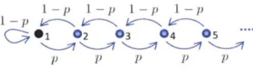
First we show an example to illustrate the limitations of local algorithms. Consider the graph shown in Figure 3.1. It is a graph with n nodes, composed of a size k clique

k uk )

k-clique (n - k + 1)-cycle

Figure 3.1. Graph of a clique plus loop

36 CHAPTER 3. ALGORITHM

connected to a size (n -k+1) cycle. Let A denote the set of nodes in the k-clique. For all nodes

j

E E \ i, let the self loop probability Pyg = . For node

j

in the clique excluding

i, let the remaining transition probabilities be uniform over the neighbors. Thus with probability 2, a random walk stays at node

j,

but with probability 1 the random walk chooses a random neighbor. For node

j

in the loop, if the random walk does not remain at node

j

with probability jthen the random walk travels counterclockwise to the subsequent node in the loop. For node i, with probability c the random walk enters the loop, and with probability

j

the random walk chooses any neighbor in the clique.

We can show that the expected return time to node i is

E[Ti] = - ) + c E[Tfirst step enters cycle] + 2 E[Tifirst step enters clique] 1

S1+ E(2(n - k)) + -I(2(k - 1)) = k + 2e(n - k) (3.1) 2

Therefore, keeping k, e fixed, as n increases,

71

= 1/E[T] decreases and scales as 0(1/n). For any fixed threshold 0, n can be chosen such that n

>

0+k. Any algorithm

that only has access to a local neighborhood of node i up to distance 0 will not be able to obtain an accurate estimate of

ri,

as it cannot differentiate between a graph having n = + k or n

>

0 + k nodes. This shows a setting in which any local algorithm

will perform poorly. For another example, see the Magnet graph in Section 6. In these examples, for any local algorithm, we can at best provide an estimate that is an upper bound for 7ri. We cannot guarantee that the estimate is close, as the true value for ni can be arbitrarily small as a function of the graph properties outside of the local neighborhood. Thus, it is impossible to have a local algorithm that is always able to determine 1ri < A or 7ri > A accurately for all nodes i c E.

Revised Problem Statement. Therefore, we consider the next natural variation of the above stated problem and answer it successfully in this thesis: for nodes with 7ri > A,

Sec. 3.2. Monte Carlo Return Time (MCRT) Algorithm 37 correctly determine that

7i

> A with high probability (with respect to randomness in the algorithm). Equivalently, when the algorithm declares that 7ri < A, then node i has 7ri < A with high probability. Note that the algorithm may incorrectly guess that

ri > A for nodes that have 7ri < A.

As discussed, the example in Figure 3.1 shows that such one-sided error is unavoid-able for any local algorithm. In that sense, we provide the best possible local solution for computing stationary distribution.

* 3.2 Monte Carlo Return Time (MCRT) Algorithm

Algorithm. Given a threshold A e (0, 1) and a node i E E, the algorithm outputs an estimate fri of rj. The algorithm relies on the relation ri= 1/lEi[T] (cf. Eq 2.3), and estimates 7ri by sampling from min(Ti, 0) for some 8 large enough. By definition, Ei [Ti] is equal to the expected length of a random walk that starts at node i and stops the moment it returns to node i. Since the length of T is possibly unbounded, the algorithm truncates the samples of T at some threshold 0. Therefore, the algorithm involves taking N independent samples of a truncated random walk beginning at node

i and stopping either when the random walk returns to node i, or when the length

exceeds 0. Each sample is generated by simulating the random walk using "crawl" operations over the Markov chain graph G.

As N -+ o and 0 - oc, the estimate will converge almost surely to ri, due to the strong law of large numbers and positive recurrence of the Markov chain (along with property (2.3)). The question remains how to choose 0 and N to guarantee that our estimate will have a given accuracy with high probability. The number of samples N

must be large enough to guarantee that the sample mean concentrates around the true mean of the random variable. We use Chernoff's bound (see Appendix 2.3.2 ) to choose a sufficiently large N, which increases with 0. Choosing 9 is not as straightforward. If

38 CHAPTER 3. ALGORITHM

O is too small, then most of the samples may be truncated, and the sample mean will be far from the true mean. However, using a large 0 requires also a large number of samples N, and may be unnecessarily expensive.

Since the algorithm has no prior knowledge about the distribution of Ti, we search for an appropriate 0 by beginning with small values for 6, and increasing the value geometrically. This is order-optimal: the final choice of 6 will be at most a constant factor more than the optimal value. Let the computation time be a function f(0). Then the total cost of executing the algorithm repeatedly for geometrically increasing values of 0 will be log0

f(2').

t=1 If f(x) is super-linear in x, then log 0 _{log 0} 2tf(2t) f(2') 2 2 ) Et 2t t=1 t=1 log 0 ()

O

2t t=1 f (0)20 * f)0 = 2f(0).

Therfore, since the computation time of our algorithm for a fixed 0 is super-linear in 0, repeating our algorithm for geometrically increasing values of 0 until we find the best 0 will cost at most 2 times the computation time of the algorithm given the optimal value for 0.

Monte Carlo Return Time (MCRT) Algorithm

Sec. 3.2. Monte Carlo Return Time (MCRT) Algorithm 39 estimate, and a = probability of failure. Set

t =,O~ -(1) = 2, N(~ - ~6(

1

+ E) ln(8/a)~

Step 1 (Gather Samples) For each k in {1, 2, 3, ...N(0}, generate independent

sam-ples Sk of min(T, 0(t)). Let p(t) fraction of samples that were truncated at 0(t,

and let

NW

T(t) -N

k=1

Step 2 (Termination Conditions) If either

(#) (1 +

)

p(t

(a) T) > A or (b) < eA,

then stop and return estimate

1

Step 3 (Update Rules) Set

0(t+1) - 2 -0(t), N(t+') -

(1

+,(t)

],

and t-t+1.

Return to Step 1.

Throughout the paper, we will refer to the total number of iterations used in the algorithm as the value for t at the time of termination. One iteration in the algorithm refers to one round of executing Steps 1-3. The total number of "steps" taken by the algorithm is equivalent to the number of neighbor queries on the network. Therefore, it is the sum over all lengths of the random walk sample paths. The total number of steps taken within the first t iterations is _ N This is used to analyze the computation time of the algorithm.

40 CHAPTER 3. ALGORITHM

The algorithm will terminate at stopping condition (a) when the estimate is smaller than '. In Lemma 4.1.3, we prove that with high probability, p^ii > g; in all iterations. Therefore, when the algorithm terminates at stopping condition (a), we know that 7ri < A with high probability. Furthermore, important nodes such that

7

ri

>

A will not terminate at stopping condition (a) with high probability. Stopping condition (b) is chosen such that the algorithm terminates when p^ is small, i.e. when very few of the sample paths have been truncated at 0(t). We will prove in Theorem 4.1.1(2) that this stopping condition will eventually be satisfied for all nodes when

0(t) > 'A. In fact, we will also prove that P(T > 0(O)) decays exponentially in ₆(t),

and thus the algorithm will terminate earlier at stopping condition (b) depending how quickly P(T > 0(t)) decays. We show in Theorems 4.2.1 and 4.3.2 that when stopping

condition (b) is satisfied, the expected error between the estimate and 7ri is small.

* 3.3 Bias correction

Our algorithm introduces a bias, as the expected truncated return time E[min(Ti, 0)] is always less than the true expected return time E[Ti]. We can partially correct for this bias by multiplying the estimate by (1 -

P(t)).

Let fr< denote the estimate after bias correction.

Ti

For graphs that mix quickly, this correction will do well, as we will show in following analyses and simulations.

Chapter 4

Theoretical Guarantees

U 4.1 Main Theorem

We state the main result establishing the correctness and convergence properties of the algorithm, and we provide an explicit bound on the total computation performed by the algorithm. We establish that the algorithm always stops in finite time. When the algorithm stops, if it outputs fri < A/(1 + c), then with high probability 7Ti < A. That is, when ri > A, the algorithm will output ri > A/(1 + c) with high probability. Thus, if we use the algorithm to identify high probability nodes with 7r, > A, then it will never have false negatives, meaning it will never fail to identify nodes that are truly important (with high probability). However, our algorithm may possibly produce false positives, identifying nodes as "high probability" even when in fact they may not be. Effectively, the false positives are nodes that are "high probability" nodes with respect to their local neighborhood, but not globally. In that sense, the false positives that the algorithm produces are not arbitrary false positives, but nodes that have high probability, "locally". As showed in the example in Chapter 3, it is impossible for any finite, local algorithm to avoid false positives entirely. In that sense, ours is as good a local algorithm as one can expect to have for general Markov chains. The following statement holds in general for all positive recurrent countable state space Markov chains. It shows a worst case dependence on the parameters chosen for the

42 CHAPTER 4. THEORETICAL GUARANTEES

algorithm and irregardless of the properties of the graph.

Theorem 4.1.1. For an aperiodic, irreducible, positive recurrent, countable state space

Markov chain, for any i

e E:

1. Correctness. When the algorithm (cf. Section 3.2) outputs -ri < A/(1 + e), then indeed 17r < A with probability at least (1 - a). Equivalently, when ,ri ;> A, the

algorithm outputs frj > A/(1 + e) with probability at least (1 - a).

2. Convergence. With probability 1, the number of iterations t in the algorithm is bounded above byl

t < In

and the total number of steps (or neighbor queries) used by the algorithm is bounded above by

~6l( )

The Markov chain is required to be aperiodic, irreducible, and positive recurrent so that there exists an unique stationary distribution. All irreducible finite state space Markov chains are positive recurrent, therefore the positive recurrence property is only explicity required and used in the analysis of countably infinite state space Markov chains. Part 1 of this theorem asserts that the estimate is an upper bound with high probability. Part 2 of this theorem asserts that the algorithm terminates in finite time as a function of the parameters of the algorithm. Both of these results are independent from specific properties of the Markov chain. In fact, we can obtain tighter charac-terizations (see sections 4.2 and 4.3) of both the correctness and the running time as functions of the properties of the graph. The analysis depends on how sharply the distribution over return times concentrate around the mean.

Sec. 4.1. Main Theorem 43 Proof of Theorem 4.1.1(1). We prove that for any node such that 7ri > A, the

algorithm will output fri > A/(1 + e) with probability at least (1 - a).

First, we prove that

it)

lies within an e multiplicative interval around E [f ] with high probability.

Lemma 4.1.2. For every t E Z+,

P(

{

T k) - ET (k) <EEi [Pk)

})

- a.

Proof. Let At denote the event

{.(t)

-

[t

< eEi .t) Since NNt) is a random

variable due to its dependence on

it

, the distribution of

i

depends on the value of

fi(t-1).

Thus, we condition on the occurrence of At_1, such that

N(t ) - 3(1 + c)6t ln(4(0)a)

Ti(t-1)E2

3(1 + c)O(t) ln(40(')/a) _ 3 0(t) ln(40(t/a) (1 + e)IEj[f(t-1)]2 - E[T(t-1)]2

Then we apply Chernoff's bound for independent identically distributed bounded ran-dom variables (see Theorem 2.3.2), substitute in for N(t), and use the facts that

Ei[Ti(t)] > Ei[fi(t-1)] and 0(t) = 2t for all t, so

Ce2 NN Ei [if (] Pi (At|At__{1) > 1 - 2exp} 3(t) Ei[t ]ln(40(t)/a) > 1 - 2exp -> 20(t)

CHAPTER 4. THEORETICAL GUARANTEES

of N(. Therefore,

;> -(I

k=1

We use the fact that ] 1 (1 - xk) >1-

>

1

xk when

Ej_

ze < 1, to show that

P2 (A)

t

> 1- -=1 - a(1 - 2-t) > 1 - a.

Next, we proceed to prove the main correctness result.

Lemma 4.1.3 (Correctness). When the algorithm outputs it < A/(1 + e), then indeed ,ri < A with probability at least (1 - a). Equivalently, when ri > A, the algorithm outputs fri > A/(1 + e) with probability at least (1 - a).

Proof. By Lemma 4.1.2, for all t, with probability (1 - a),

i0 < (1 E)E± [ ]. By definition of Ei[fit)], E [T$t)] <E [T]. Therefore, r > - 1 + E

If frj < A/(1 + e), then

ri

A

1+e 1+e #-7 < A. 2k+1) U (4.1) 0 44 Pi (At|lAt_1) Pi

nA

= Pi (A1) r \k=1 / k=2