Publisher’s version / Version de l'éditeur:
Vous avez des questions? Nous pouvons vous aider. Pour communiquer directement avec un auteur, consultez la première page de la revue dans laquelle son article a été publié afin de trouver ses coordonnées. Si vous n’arrivez pas à les repérer, communiquez avec nous à [email protected].
Questions? Contact the NRC Publications Archive team at
[email protected]. If you wish to email the authors directly, please see the first page of the publication for their contact information.
https://publications-cnrc.canada.ca/fra/droits
L’accès à ce site Web et l’utilisation de son contenu sont assujettis aux conditions présentées dans le site LISEZ CES CONDITIONS ATTENTIVEMENT AVANT D’UTILISER CE SITE WEB.
Technical Report, 2004
READ THESE TERMS AND CONDITIONS CAREFULLY BEFORE USING THIS WEBSITE. https://nrc-publications.canada.ca/eng/copyright
NRC Publications Archive Record / Notice des Archives des publications du CNRC :
https://nrc-publications.canada.ca/eng/view/object/?id=7316ea99-f289-41a3-8a1a-999cfbff733c https://publications-cnrc.canada.ca/fra/voir/objet/?id=7316ea99-f289-41a3-8a1a-999cfbff733c
NRC Publications Archive
Archives des publications du CNRC
For the publisher’s version, please access the DOI link below./ Pour consulter la version de l’éditeur, utilisez le lien DOI ci-dessous.
https://doi.org/10.4224/8896297
Access and use of this website and the material on it are subject to the Terms and Conditions set forth at
Terry Fox resistance tests - Phase III (PMM) ITTC Experimental Uncertainty Analysis Iniative
DOCUMENTATION PAGE REPORT NUMBER
TR-2004-05
NRC REPORT NUMBER DATE
April 2004
REPORT SECURITY CLASSIFICATION
Unclassified
DISTRIBUTION
Unlimited
TITLE
Terry Fox Resistance Tests – Phase III (PMM) Testing ITTC Experimental Uncertainty Analysis Initiative
AUTHOR (S)
Ahmed Derradji-Aouat and Amy van Thiel
CORPORATE AUTHOR (S)/PERFORMING AGENCY (S)
Institute for Ocean Technology, National Research Council
PUBLICATION
SPONSORING AGENCY (S)
Institute for Ocean Technology, National Research Council
IMD PROJECT NUMBER
42_953_10
NRC FILE NUMBER KEY WORDS
Ship, Icebreaker, Resistance, Experimental Uncertainty Analysis, Ice, ITTC, Tank, Pack ice, Standards, Planar Motion Mechanism, Manoeuvring.
PAGES vi, 22, App. 1-7 FIGS. 25 TABLES 12 SUMMARY:
This is the 3rd phase of a research program designed to develop a procedure for Experimental Uncertainty Analysis (EUA) for ship resistance testing in an ice tank. The latter is a task for the 23rd and 24th ITTC specialist committee on ice.
In this report, the results of Phase III ship resistance in ice test program were documented and used to formulate the EUA procedure. One of the objectives of Phase III test program is to compare the test results using the tow post (Phase I) with those using the PMM (Phase III).
The procedure for EUA, presented in this report, validates the applicability of the preliminary EUA procedure (previously, proposed by Derradji-Aouat, 2002) to the laboratory measurements from both phases of testing. Consequently, this EUA procedure will be recommended to the 24th ITTC (during its upcoming meeting in Scotland, 2005).
ADDRESS National Research Council
Institute for Ocean Technology Arctic Avenue, P. O. Box 12093 St. John's, NL A1B 3T5
National Research Council Conseil national de recherches
Canada Canada
Institute for Ocean Institut des technologies
Technology océaniques
TERRY FOX RESISTANCE TESTS – PHASE III (PMM) TESTING
ITTC EXPERIMENTAL UNCERTAINTY ANALYSIS INITIATIVE
TR-2004-05
Ahmed Derradji-Aouat and Amy van Thiel
TABLE OF CONTENTS
List of Tables ...v
List of Figures ... vi
1. INTRODUCTION... 1
2. EXPERIMENTAL UNCERTAINTY ANALYSIS (EUA)... 2
2.1 BASIC FORMULATION... 2
2.2 UNCERTAINTY COMPONENTS AND BIAS EFFECTS IN ICE TANK TESTING... 2
3. TEST SETUP ... 3
4. DATA ACQUISITION SYSTEM (DAS)... 3
5. INSTRUMENTATION AND CALIBRATIONS... 4
6. DESCRIPTION OF THE EXPERIMENTAL PROGRAM ... 4
6.1 ICE TYPE AND ICE PROPERTIES... 4
6.2 TEST MATRIX AND RUN SEQUENCE... 4
6.3 DESCRIPTION OF THE EXPERIMENTS IN ICE... 5
6.4 DESCRIPTION OF THE EXPERIMENTS IN OPEN WATER... 6
7. DATA STORAGE AND RESISTANCE CALCULATIONS ... 7
8. PHASE III RESULTS ... 7
8.1 RESISTANCE IN BASELINE OPEN WATER TESTS... 7
8.2. RESISTANCE IN STANDARD OPEN WATER TESTS... 7
8.3 RESISTANCE IN ICE TESTS... 8
8.4 COMPARISON OF TEST RESULTS... 8
8.4.1 Tow Force in Baseline Open Water Tests... 8
8.4.2 Resistance in Standard Open Water Tests ... 8
8.4.3 Resistance in Ice Tests ... 8
9. COMPONENTS FOR SHIP MODEL RESISTANCE IN ICE... 9
10. EUA FOR ICE TANK TESTING – A PROCEDURE DEVELOPMENT.... 10
10.1 SEGMENTATION HYPOTHESIS... 10
10.2 STEADY STATE REQUIREMENTS... 12
10.2.1 Effects of changing carriage speed... 13
10.2.2 Effects of non-uniform ice thickness ... 13
10.2.3 Effects of non-homogeneous ice properties ... 15
11. CALCULATIONS FOR RANDOM UNCERTAINTIES ... 16
11.1 RANDOM UNCERTAINTIES IN MEAN TOW FORCE... 18
11.2 RANDOM UNCERTAINTIES IN MAXIMUM TOW FORCE... 18
11.3 EFFECT OF CORRECTION FOR ICE THICKNESS ON RANDOM UNCERTAINTIES... 19
11.4 EFFECTS OF DATA REDUCTION EQUATION... 19
11.5 COMPARISON OF UNCERTAINTIES IN CONTINUOUS ICE AND IN BROKEN ICE... 20
11.6 COMPARISON OF UNCERTAINTIES IN MEAN AND MAXIMUM TOW FORCES... 20
12. BIAS AND TOTAL UNCERTAINTIES ... 20
13. COMPARISON OF PHASE I AND III UNCERTAINTIES... 20
13.1 UNCERTAINTIES IN MEAN RESISTANCE... 21
13.2 UNCERTAINTIES IN MAXIMUM RESISTANCE... 21
14. SUMMARY, CONCLUSIONS AND RECOMMENDATIONS ... 21
15. REFERENCES... 21
APPENDIX 1: Hydrostatics and Particulars of the Terry Fox model APPENDIX 2: Instrumentation and Calibration
APPENDIX 3: Ice Sheet Summaries and Ice Properties
APPENDIX 4: Test Matrix, Run Sequence and File Naming Convention APPENDIX 5: Typical Test Results
APPENDIX 6: Analysis of the Spatial Distribution of the Properties of Model Ice In the IOT Ice Tank
APPENDIX 7: Comparison of the Tow Post (Phase I) and the PMM (Phase III) Test Results and Uncertainties
LIST OF TABLES
Table
% Difference in Phase I and Phase III measured Mean Tow Force ...1
% Difference in Phase I and Phase III measured Maximum Tow Force...2
Slope for tow force time histories...3a Change in measured tow force during test run ...3b Slope for carriage speed time histories ...3c Change in measured carriage speed during test run ...3d Ice Sheet Thickness Data and experimental uncertainty calculations ...4
Ice Flexural Strength components ...5
Ice density components...6
Random Uncertainties in Mean Tow Force ...7
Random Uncertainties in Maximum Tow Force ...8
Corrected Mean of Means in Tow Force ...9a Random uncertainties in corrected mean tow force before DRE ...9b Random uncertainties in corrected mean tow force after DRE ...9c Corrected Mean of Maximums in Tow Force...10a Random uncertainties in corrected maximum tow force before DRE ...10b Random uncertainties in corrected maximum tow force after DRE...10c Comparison of Phase I and III Experimental Uncertainties in Mean Tow Force...11
Comparison of Phase I and III Experimental Uncertainties in Maximum Tow Force ...12
LIST OF FIGURES
Figure Tow post test setup...1a Planar Motion Mechanism test setup...1b
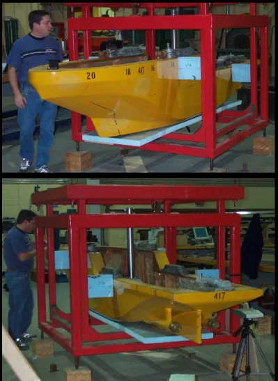
Terry Fox model (IMD model # 417) in the preparation shop ...2
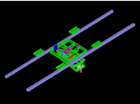
Actual Planar Motion Mechanism on the shop floor ...3a Planar Motion Mechanism Planar isometric top view...3b Actual Planar Motion Mechanism (top view)...3c Planar Motion Mechanism top and bottom CAD views...3d A schematic for Run # 1, Run # 2 and Run # 3 ...4
Typical test run in continuous ice (Phase III) ...5a Typical test run in broken ice (Phase III)...5b Phase III results from baseline open water tests – measured tow force vs. velocity ...6a Phase III results from standard open water tests – measured tow force vs. velocity...6b Measured tow force in continuous ice test runs...7a Measured tow force in broken ice test runs ...7b Baseline open water tests (comparison between phases I, II and III)...8a Baseline open water tests (best fit for all phases of testing) ...8b Standard open water tests (comparison between phases I, II and III) ...9a Standard open water tests (best fit for all phases of testing)...9b Comparison of Phase I and Phase III measured mean tow force...10a Comparison of Phase I and Phase III measured maximum tow force ...10b Measured tow force vs. time and measured speed vs. time example ...11
Measured tow force versus time ...12
Measured speed versus time ...13
Thickness profiles ...14
Corrected versus measured mean tow force ...15
Corrected versus measured maximum tow force...16
Flexural strength profiles ...17
Ice density profiles...18
Mean of means of corrected tow force ...19
Mean of maximums of corrected tow force ...20
Uncertainty in the mean of means for tow force...21
Uncertainty in the mean of maximums for tow force ...22
Effect of correction on uncertainty in ice resistance for ice thickness variations...23
Uncertainties in maximum tow forces versus mean tow force after DRE...24 Comparison of Phase I and III uncertainty in mean tow force after DRE...25a Comparison of Phase I and III uncertainty in maximum tow force after DRE ...25b
Terry Fox Resistance Tests – Phase III (PMM)
ITTC Experimental Uncertainty Analysis Initiative
1.
Introduction
Experiments for ship model resistance in ice were conducted at the Institute for Ocean Technology of the National Research Council of Canada (www.iot-ito.nrc-cnrc.gc.ca/). These tests were conducted for the ITTC 23rd and 24th specialty committee on ice1 (mandate period 1999-2002 and 2002-2005, respectively). One of the committee’s main objectives is to develop a procedure for Experimental Uncertainty Analysis (EUA) in ice tank testing. So far, three phases of testing have been completed. From project management point of view, the Terry Fox test program was divided into several phases to accommodate the project planning for opportunity testing in the ice tank.
In this report, Phase III test program, test results, and calculations of uncertainties in the test results are presented. However, for clarity and completeness, the following short summary regarding all three phases of the test program is given.
Phase I test program was documented by Derradji-Aouat et al. (2002) and Derradji-Aouat (2002) in two (2) internal technical reports: These are: TR-2002-01 and TR-2002-04, the first report dealt with presenting the experimental program and test results, while the second report dealt with developing a preliminary methodology to quantify Experimental Uncertainties (EU) in the test results.
Similarly, the documentation for Phase II testing program is presented in two (2) internal reports (Derradji-Aouat and Coëffé, 2003, and Derradji-Aouat, 2003). In the first report, Phase II test program and test results are presented. In the second report calculations for EU in Phase II test results are given. Note that both reports provide comparisons between Phase I and Phase II test results.
In Phase II, the same test matrix as in Phase I was repeated. The only difference is the target thickness of the ice sheets. In Phase I, all tests were conducted for only one target ice thickness (40 mm), while Phase II tests were conducted for two additional target ice thicknesses (25 mm and 55 mm). In a way, Phase II test program is a continuation of Phase I. Together, both phases provided information for three different ice sheet thicknesses.
In Phase III, the same test matrix as in Phase I was completed. All tests were conducted for only one target ice thickness (40 mm). The difference between phase I and phase III test programs is that in phase I, the model was attached to the carriage using the tow post (Figure 1.a), while in phase III, the model was attached to the carriage using the PMM (Planar Motion Mechanism, Figure 1.b). One of the objectives of phase III test
1
ITTC = International Towing Tank Conference
program is to compare test results using the tow post (Phase I) with the test results using the PMM (Phase III).
In all phases of testing, tests in ice involved a total of sixteen (16) different ice sheets. Phase I of testing required four (4) different ice sheets, all four ice sheets had nominal thickness of 40 mm and nominal flexural strength value of 35kPa. Phase II of testing, however, required eight (8) different ice sheets, four ice sheets had nominal thickness of 25 mm and the other four ice sheets had nominal thickness of 55 mm. All Phase II ice sheets had nominal flexural strength value of 35 kPa. Phase III of testing required four (4) different ice sheets, all four ice sheets had nominal thickness of 40 mm and target nominal flexural strength value of 35kPa.
All phases involved experiments in both ice and calm open water. In all phases, all experiments were conducted using a model for the Canadian Icebreaker, “Terry Fox”, shown in Figure 2. The latter is the IOT standard icebreaker model (IOT Model # 417, scale ≈1:21.8), its particulars and hydrostatics are given in Appendix 1. During Phases I and II, the ship model motions (heave, pitch and roll), tow force and carriage speed were measured. The same parameters were measured during Phase III, with the exception of roll (PMM tests were fixed in roll). During Phase III, sway and yaw were also measured.
2.
Experimental Uncertainty Analysis (EUA)
A literature review for the history and development of EUA in marine/ocean testing facilities was given by Derradji-Aouat (2002).
2.1 Basic Formulation
Mathematically, the EUA procedure presented in this report is based on the equations provided by Coleman and Steel (1998). The latter is in harmony with the guidelines of ISO (1995), ASME (PTC-19.1, 1998), and GUM (2003).
2.2 Uncertainty Components and Bias Effects in Ice Tank Testing
In a typical experiment, the total uncertainty (U) is the geometric sum of a bias uncertainty component (B) and a random uncertainty component (P):
(
B P)
U = ± 2 + 2 (1a) The bias component (B) deals with uncertainties in instrumentation and equipment calibrations. Examples of bias uncertainty sources are the load cells, RVDT’s (Rotary Variable Differential Transformers), yoyo potentiometers and Data Acquisition System (DAS). However, the precision component (P) deals with environmental and human factors that may effect the repeatability of the test results (i.e. if a test was to be repeated several times, would the same results be obtained each time?). Examples of random uncertainty sources are the changing test environment (such as fluctuations in room temperature during testing), small misalignments in the initial test setup, human factors, …etc.
Derradji-Aouat (2002) showed that in a typical ice tank ship resistance test, the bias uncertainty component (B) is much smaller than the random one (P), he reported that, in Phase I ship model tests in ice, the value of (B) is at least one order of magnitude smaller than the value of (P). He concluded, therefore, that; in routine ship resistance ice tank testing, the total uncertainty (U) can be taken as equal to the random one. Simply, without a loss of accuracy, the bias uncertainty component can be neglected. It follows that:
P
U
=
±
(1b)3. Test
Setup
In these tests, the main components of the test set up are: The Terry Fox ship model, the PMM (Figure 3), data acquisition system (DAS) and video cameras.
Marineering Limited (1997) provided details on the development and commissioning of the PMM. Originally, the PMM was designed to study maneuvering of ships in both ice and open water. The PMM dynamometer has 4 cantilever type load cells for measuring surge force, sway force and yaw moment. Surge is measured by two load cells aligned along the x-axis. Sway force is measured by two other load cells aligned along the y-axis. Yaw moment is determined by all four load cells.
4.
Data Acquisition System (DAS)
Eleven channels were used to record the data. The test program required measurements of the following 11 items:
i. FWD Sway (N)……… Channel # 2.
ii. AFT Sway (N)………. Channel # 3.
iii. Surge Center 2 (N)……….…………. Channel # 4.
iv. X-Pull (N)……… Channel # 5.
v. Y-Pull (N)……… Channel # 6.
vi. Yaw (degrees).……….………… Channel # 9.
vii. FWD Heave (mm)………..……….……… Channel # 10.
viii. AFT Heave (mm).………... Channel # 11.
ix. Pitch (degrees).……… Channel # 28.
x. Carriage Position (ITC o/p) (m)……….. Channel # 31. xi. Carriage Velocity (ITC o/p) (m/s)………... Channel # 32.
All acquired analog DC signals were low pass filtered at 10 Hz., amplified as required and digitized at 50 Hz. (details given at the IOT quality system standard document for Data Acquisition, Verification and Storage, IOT standard # 42-8595-S/GM-2).
In this project, it was required that all measurements need to be accurate to about ± 2% of the instrumentation range (specifications are given in the Project Initiation Plan “PIP” document).
5.
Instrumentation and Calibrations
All details regarding the instrumentations used in this test program and their calibration sheets are given in Appendix 2.
6.
Description of the Experimental Program
6.1 Ice Type and Ice Properties
The program required four (4) different ice sheets. Non-bubbly ice was used. The procedures followed to prepare the ice tank, seed and grow the ice sheet are given in the IOT work procedures TNK 22, TNK 23, and TNK37, respectively. All work procedures are given in the IOT documentations for the quality system.
The mechanical properties of the ice are determined according to the following work procedures: TNK 26 (for measurements of the flexural strength), TNK 27 (for measurements of the elastic modulus), TNK 28 (for measurements of the compressive strength), and TNK 30 (for measurements of the ice density).
Measurements of ice thickness are performed as per the work procedure TNK 25. A summary of the ice sheets (seeding, growth and warm-up) and the measurements of the necessary ice properties, tempering curves, and schematics for the location of ice samples used for the flexural strength tests are presented in Appendix 3 (summaries for all 4 ice sheets are included).
It should be noted that all of the above work procedures are valid for both bubbly ice and non-bubbly ice. Simply, in the case of non-bubbly ice, the bubbler system is not used (the bubbler system is turned off).
6.2 Test Matrix and Run Sequence
The overall test matrix is given in Appendix 4. Broadly speaking, two (2) different types of experiments were performed. These are experiments in ice and experiments in open water.
• Experiments in Ice:
1.a: Experiments in level ice sheets (continuous, unbroken ice sheets). 1.b: Experiments in pre-sawn ice sheets.
1.c: Experiments in pack ice (broken ice, the ice sheet was broken, manually, and ice blocks were re-distributed in the tank to achieve various ice concentrations).
All tests in ice were conducted with no turbulent stimulation studs.
• Resistance Experiments in Open Water:
2.a: Standard resistance experiments in open water (ship model is equipped with turbulent stimulation studs and beach absorbers were used).
2.b: Baseline experiments in open water (constant speed through the length of the tank, turbulent stimulation studs were not used).
Note that all of the open water tests were conducted in the ice tank, for calm water conditions (no waves).
6.3 Description of the Experiments in Ice
The test program involved the use of four (4) different ice sheets. All ice sheets had the same target thickness (40 mm) and the same target flexural strength (35 kPa). All tests were conducted at approximately 0°C air temperature.
As indicated in Appendix 4, ship model speeds of 0.1 m/s, 0.2 m/s, 0.4 m/s and 0.6 m/s were selected. Each ice sheet was tested for only one speed. Ice sheet # 1 was tested for speed of 0.1 m/s, ice sheet # 2 was tested for speed 0.2 m/s, ice sheet # 3 was tested for speed of 0.4 m/s and ice sheet # 4 was tested for speed 0.6 m/s.
In each ice sheet, six (6) different test runs were performed. The first three runs were conducted in continuous “unbroken” ice, while the last three runs were conducted in pack “broken” ice.
Figure 4 shows a schematic for the first three (3) test runs:
Run # 1: This run was performed in a level “unbroken” ice sheet, along the centerline of the tank (central channel, CC). The carriage speed was kept constant along most of the entire useable length of the ice tank (the entire usable length is ≈ 76 m, each test run uses ≈ 65 m).
Note that after the completion of Run # 1, an open water channel along the centerline of the tank is created.
Run # 2: After the completion of the first run, the model was moved to the South Quarter Point (SQP) of the tank. The south half of the ice sheet was constrained (using pegs), and the ice was pre-sawn along the SQP straight path. A resistance test run was performed in the pre-sawn ice at constant speed (same speed as Run # 1) along most of the entire useable length of the ice tank.
Run # 3: The model was moved to the North Quarter Point (NQP) of the tank. The north half of the ice sheet was neither pre-sawn nor constrained (no pegs, the ice sheet had a free boundary). Resistance test run was performed in the ice sheet at constant speed (same speed as Run # 1) along most of the entire useable length of the ice tank.
The last three runs (Runs # 4, # 5 and # 6) were performed in broken ice. After the completion of the first three runs, the ice sheet was broken (manually) into small blocks (the ice was broken slowly to avoid rafting) with arbitrary shapes. The ice blocks were re-distributed in the tank, manually, to achieve the desired pack ice concentration. Three (3) different pack ice concentrations were targeted; these are the 9/10ths, 8/10ths and 6/10ths. These ice concentrations were chosen to reflect actual “existing” pack ice environment. Note that ice concentration less than about 6/10th yields behavior equivalent to that of baseline open water tests.
The three test runs in pack ice are:
Run # 4: Test run in 9/10ths ice concentration. The ship model was towed along the NQP at a constant speed (same speed as in Run # 1).
Run # 5: Test run in 8/10ths ice concentration. The model was towed along the CC of the ice tank at a constant speed (same speed as in Run # 1).
Run # 6: Test run in 6/10ths ice concentration. The ship model was towed along the SQP at a constant speed (same speed as in Run # 1).
After the completion each test run, a creeping test was performed in the remaining portion of the ice sheet. A creeping test run is a resistance test at very low ship speed (≈ 0.02 m/s) for at least one ship length.
The above six test runs (Run # 1 to Run # 6) were repeated for each ice sheet, with the exception of the first ice sheet (Run # 6 was not completed due to time constraints). A total of 23 resistance test runs in ice were conducted.
Figures 5a and 5b show pictures of typical test runs in ice. 6.4 Description of the Experiments in Open Water
• Standard Resistance Experiments in Open Water:
Six (6) standard open water resistance tests were performed in the ice tank. In all six tests, turbulent stimulation studs were placed on the model. Also, beach absorbers were used. In these test, ship speeds from 0.3 m/s to 1.7 m/s were covered.
• Baseline Resistance Experiments in Open Water:
For these tests, the turbulent studs and beach absorbers were removed. In each test, the model was towed in calm open water at constant velocity along the entire length of the ice tank (same as in the case for ice tests). Velocities of 0.1 m/s, 0.2 m/s, 0.4 m/s and 0.6 m/s were selected. Tests for each velocity were repeated several times (see test matrix in Appendix 4). A total of (26) baseline open water resistance tests were conducted.
7.
Data Storage and Resistance Calculations
All test results (data-files and test plots) are stored in the IOT computer system under the directory name “PJ02953” on Mickey server.
A summary of the completed test matrix and the data file naming convention are given in Appendix 4.
Plots for typical test results are given in Appendix 5. These plots include: • Typical results for resistance experiments in ice:
P3_S3_NQP_R3_0P4_038
• Typical results for the baseline resistance experiments in open water: P3_OW_V8_008
• Typical Results for the standard resistance experiments in open water: P3_OW_V2_082
8.
Phase III Results
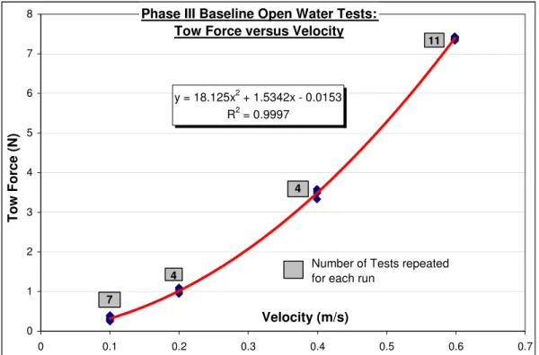
8.1 Resistance in Baseline Open Water Tests
The test results are given in Figure 6a. The numerical values for the mean tow force at each speed are:
Model velocity (m/s) 0.1 0.2 0.4 0.6
Number of tests repeated 7 4 4 11
Mean Tow Force (N) 0.319371 1.016385 3.4846 7.392555
Standard deviation 0.053471 0.066705 0.109116 0.032734
The resistance in baseline open water tests (RBaseline) is obtained from the
regression line in Figure 6a:
(
RBaseline)
= 18.125 *V2 + 1.5342 *V − 0.0153 (2a) 8.2. Resistance in Standard Open Water TestsFigure 6b shows the results from the six different tests conducted in the ice tank. The resistance (RSTD_OW) is obtained from the regression line in Figure 6b:
(
RSTD_OW)
= 42.343 *V2 − 34.193 *V + 11.573 (2b)8.3 Resistance in Ice Tests
• Tow Force versus velocity in continuous ice
Figure 7a shows the measured tow force versus velocity curves for all tests in continuous ice (Runs # 1, 2 and 3). All curves exhibit the same general trends. • Tow Force versus velocity in broken ice
All measured tow force versus velocity curves in broken ice tests are given in Figure 7b. The results show that the 9/10ths and 8/10ths ice coverage tests, resistance curves are almost linear (very low level of non-linearity). However, in the 6/10ths ice coverage, the tow force versus velocity curves are highly non-linear (approach open water resistance in Fig. 6a).
8.4 Comparison of Test Results
8.4.1 Tow Force in Baseline Open Water Tests
• Comparison between tests from Phases I, II and III
The general trend of the curves for resistance versus model speed is the same for both phases (Figures 8a and 8b). The differences in mean resistances for Phases I and III are:
Approx. Speed
Phase I Mean Tow Force
Phase III Mean Tow Force % Difference 0.1 0.319371429 0.613016 62.99% 0.2 1.016385 1.0396 2.26% 0.4 3.4846 3.5894 2.96% 0.6 7.392554545 7.6602 3.56%
Note that for all tests, except for tests at a speed of 0.1 m/s (an outlier), there is a very small difference between the results from the two phases. At very low speed (0.1 m/s), it appears that noise levels are too high. This data point is considered an outlier.
8.4.2 Resistance in Standard Open Water Tests
• Comparison between tests from Phases I and III
Figures 9a and 9b provides a comparison between the measured tow force values in Phases I, II and III, each is plotted for tow force versus velocity. There is no significant difference between the results in all phases.
8.4.3 Resistance in Ice Tests
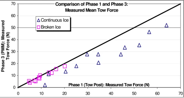
Tables 1 and 2 present the mean and maximum tow forces measured in Phases I and III, respectively. Figures 10a and 10b provide a comparison between the measured tow forces in Phase I testing and those from Phase III testing. Implicitly, the tables show the effects of the tow post and PMM on the test results. The main conclusions drawn from the comparisons are:
• Mean Tow Forces
From Table 1, mean tow forces for Phase I are generally larger than the Phase III values (Figure 10a). The difference averages 22.22% and ranges from 5.38% to 50.15%. However, at tow forces less than 20N, no significant difference is observed.
• Maximum Tow Forces
In Table 2, maximum tow forces for Phase I are generally smaller than the Phase III values (Figure 10b). The difference averages 26.6% and ranges from 1.79% to 51.09%. At tow forces lower than 100N, no significant difference is observed.
The source of the differences in the measured tow forces in Phase I and those in Phase III is, basically, unknown. However, one possibility is the effects of the test set up (the PMM test set up is much different than that of the tow post). Another possibility is that the PMM is not rigid enough as compared to the tow post.
9.
Components for Ship Model Resistance In Ice
Since the objective of the test program is to develop a procedure for EUA-ship resistance tests in ice tanks, a summary of the resistance calculations is given in this section.
The standards for ship resistance in ice (ITTC-4.9-03-03-04.2.1) and (IOT/42-8595-S/TM7) give formulas for the total resistance in ice as the sum of four individual components: R R R R Rt = br + c + b + ow (3a) where Rt is the total resistance, Rbr is the resistance component due to breaking the ice,
Rc is the component due to clearing the ice, Rb is the component due to buoyancy of the
ice and Row is the resistance in open water. In order to quantify each component, the
following test plan is to be conducted (ITTC-4.9-03-03-04.2.1):
Standard open water tests provide values for Row, while the creeping speed tests give Rb:
R
Rt = ow (in standard open water tests),
b t R
R = (in the creeping speed tests) (3b) In the pre-sawn ice tests (Runs #2), the ice breaking component Rbr = 0, and therefore:
R R R
Rt = c + b + ow (in pre-sawn ice tests) (3c) Since both Row and Rb are already known from Eq. 3b, Rc is:
R R R
Rc = t − b − ow (3d) where Rt, in Eq. 3d, is the measured resistance in the pre-sawn ice test runs.
From tests in level ice sheets, the total resistance Rt is measured, and the ice
breaking component, Rbr, is calculated as (from Eq. 3a):
R R R R Rbr = t − c − b − ow (3e) where Rt, in Eq. 3e, is the measured resistance in the level continuous ice (Run #1 tests).
Theoretically, in the ship ice resistance main equation (Eq. 3a), the superposition principle is used, which implies that the total resistance in ice is equal to the sum of four separate components. One may argue against the use of the superposition principle and the applicability of Eq. 3a to actual ship-ice interactions (since ice breaking and clearing processes are highly non-linear and dynamic, and superposition principles are applied to linear and static problems). However, this argument is beyond the scope of this report.
10.
EUA for ice tank testing – A Procedure Development
10.1 Segmentation Hypothesis
For the ice test runs, several reasons have contributed to the decision for keeping the speed of the ship model constant throughout most of the useable length of the ice tank (≈ 65 m). The main one is the hypothesis that the time history from one long ice test run can be divided into segments, and each segment can be analyzed as a statically independent test. The hypothesis states that (Derradji-Aouat, 2004):
“The history for a measured parameter (such as tow force versus time) can be divided into 10 (or more) segments, and each segment is analyzed as a statistically independent test. Therefore, the 10 segments in one long test run in ice are regarded as 10 individual (independent but identical) tests.”
Coleman and Steel (1998) reported that, in statistical uncertainty analysis, a population of at least 10 measurements (10 data points) is needed. Precision uncertainty is calculated using the mean and the standard deviation of that population.
However, in ice tank testing, it is recognized that conducting the same test 10 times is very costly and very time consuming. Therefore, the principle of segmenting a time history of a measured parameter over a long test run (such as 65 m) into 10 (or more) segments, results in significant savings in project costs and efforts. By demonstrating that each segment can be analyzed as a statistically independent test, uncertainties are calculated from the means and standard deviations of the individual segments.
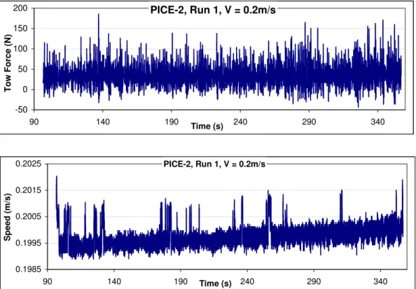
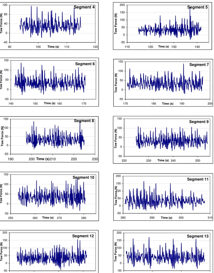
To further illustrate the segmentation hypothesis, an example is given in Figure 11. In the example, the measured tow force history in test run # 1 (nominal speed of 0.2
m/s) in ice sheet # 2 of Phase III (nominal ice thickness of 40 mm) is presented to illustrate the basic steps followed to develop the procedure on how to calculate the uncertainties in ice tank testing. The time history given in Figure 11a was divided into 10 equal (more or less equal) segments, as illustrated in Figures 11b.
In this report, only calculations of uncertainties in measured tow forces (given in Figure 11a) are presented. The same calculation steps are valid for all other measured parameters (heave, pitch, carriage speed, yaw, sway).
Using the tow force segments, in Fig. 11b, the first calculation step is to obtain mean and standard deviation for each segment. The second step is to calculate the mean of the means and the standard deviation of the means. The mean of the means and standard deviation of the means are needed to compute random uncertainties in the results of the test run (as it will be shown in the subsequent sections). These two basic calculations steps are repeated for all six (6) test runs (Run # 1 to Run # 6), in all four (4) ice sheets.
It should be cautioned that the segmentation hypothesis is valid only if the following three conditions are satisfied (Derradji-Aouat, 2004):
1. Each segment should span over 1.5 to 2.5 times the length of the ship model, 2. Each segment should include at least 10 events for ice breaking (10 load peaks) or
at least 10 collision events (in the case of pack ice test runs), and
3. General trends (of a measured parameter such as tow force versus time) are repeated in each segment.
Condition # 1 is based on the fact that the ITTC procedure for resistance tests in level ice (ITTC-4.9-03-03-04.2.1) requires that a test run should span over at least 1.5 times the model length. For high model speeds (> 1 m/s), however, the ITTC procedure requires test spans of 2.5 times the model length.
Condition # 2 is based on the fact that in EUA, for an independent test, a population of at least 10 data points is needed to achieve the minimum value for the factor t (in the t distribution Table A.2, Coleman and Steele, 1998). For tests in ice tanks, 10 to 15 segments are recommended. The gain in any further reduction in the value of t (by having more than 10 to 15 segments) is minimum.
Condition # 3 is introduced to ensure that the overall trends in a measurement (such as tow force versus time) are repeated in each segment. This condition serves to provide further assurance into the main hypothesis (“…Therefore, the 10 segments in one long test run are regarded as 10 individual, independent but identical, tests”). Fundamentally, if the trends are not, reasonably, repeated, then the segments could not be analyzed as “independent but identical” tests.
It is important to emphasize the fact that the division of the time history of a measured parameter into consecutive segments is valid only for long test runs at constant
speed and heading. If the model speed or heading is changed during the test run, then the segments cannot be analyzed as “identical”.
Note that the time histories measured in creeping speed test are not subjected to the segmentation hypothesis.
Furthermore, it is recognized that the division of the results of a test run into segments is valid only for the steady state portion of the measured data. Only, the steady state portion of the measured time history is to be used. This is required to eliminate the effects of the initial ship penetration into the ice (transient stage) and the effects of the slowdown and full stop of the carriage during the final stages of the test run.
10.2 Steady State Requirements
In ice tank testing, for any given ice sheet, the ice properties are not completely (100%) uniform (same thickness) and homogeneous (same mechanical properties) all over the ice sheet. This is attributed, mainly, to the ice growing processes and refrigeration system in the ice tank. An example to illustrate the special variability of the material properties is given in Appendix 6.
In addition to the spatial variability of the material properties of ice, during an ice test run, the carriage speed may (or may not) be maintained at exactly the required nominal constant speed2. Because of this inherent uniformity of ice sheets, the non-homogeneity of ice properties and the small fluctuations in the carriage speed, steady state condition in the time history of a measurement may not be achieved. For example, in Fig. 11, the tow force did not become completely steady after the initial transient stage. Theoretically, if the time history of a measured parameter is changing drastically, then the segments could not be analyzed as “identical” tests (condition # 3). The steady state requirement, therefore, calls for a corrective action to account for the effects of non-uniform ice thickness, non-homogenous ice mechanical properties and small fluctuations in carriage speed on the test measurements.
To identify whether or not the time history for a measured parameter has reached its steady state, the following procedure was recommended (Derradji-Aouat, 2002). The measured time histories for all parameters, in all 23 ice test runs, were plotted along with their linear trend lines. A linear trend line with zero slope (or very close to zero) indicates that a steady state in a measured parameter is achieved.
So far, in this project, all three phases of testing generated a total of 498 time histories (there are 95 ice test runs, and in each test run five parameters are measured for Phases I and II3 and six parameters are measured in Phase III4). For example, Fig. 12
2
The control system maintains the carriage speed constant. However, when ice breaks, small fluctuations in carriage speed may take place.
3
Tow force, carriage speed and three ship model motions (heave, pitch and roll).
4
Tow force, carriage speed and four ship model motions (heave, pitch, sway and yaw).
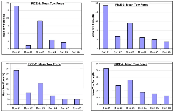
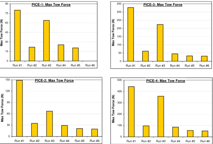
shows the time histories for the measured tow forces in Phase III testing. Time histories for Phases I and II testing were provided in previous reports by Derradji-Aouat (2002) and Derradji-Aouat (2003), respectively.
After drawing the linear trend lines through all measured tow forces, it was observed that, in the majority of cases, a true steady state was never achieved (Table 3a). For example, the linear trend lines (in Fig. 12) show that the tow force time histories runs changed over a range of 0.002% (for PICE-2 – Run # 3) to 5.2% (for PICE-4 – Run # 1). The sloping trend lines reflect the fact that the time histories never reached their steady state.
As shown in Table 3b, it is interesting to show that, although the slopes of the trend lines varied within only 5.2%, they led to some significant changes in the tow forces over the 65 m towing distance (up to 121% in PICE-1, Run # 5).
Therefore, in this work, it is suggested that the non-steady state condition may be attributed to one (or all) of the following three factors:
i. A changing carriage speed (or small fluctuations in carriage speed) during testing, ii. Non-uniform ice thickness,
iii. Non-uniform mechanical properties of the ice (flexural/compressive strengths, elastic modulus and density of ice).
The contribution of each factor is further investigated as follows: 10.2.1 Effects of changing carriage speed
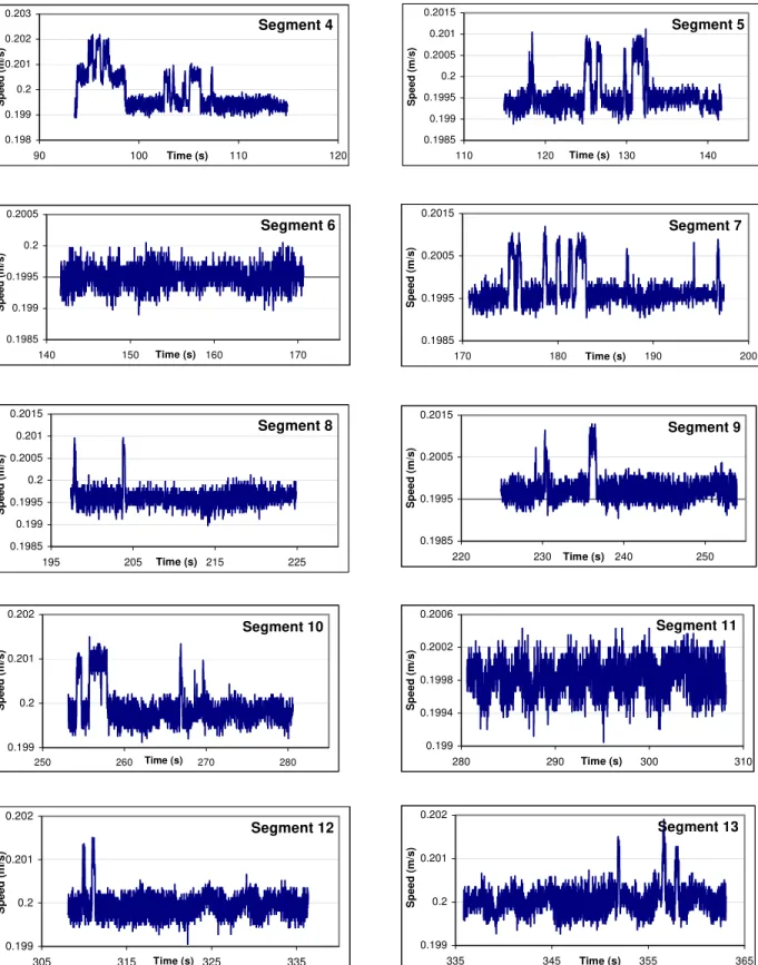
Figure 13 shows the time histories for the measured carriage speed histories in Phase III testing. The results, for Phases I and II testing, were already given by Derradji-Aouat (2002, 2003). The linear trend lines point to the fact that, during testing, the actual changes in the carriage speeds were very small, and consequently, they can be neglected. Trend lines through the carriage speed histories had slopes between 1 X 10⁻⁸ (for PICE-3 - Run # 5) to 6 X 10⁻⁶ (for PICE-4 - Run # 3). Table 3d shows that, over the ≈ 65 m towing distance, changes in the carriage speed ranged between 0.0003% (PICE-3, Run # 5) and 0.53% (PICE-1, Run # 1) with a mean of about 0.18%.
Over the ≈ 65 m towing distance, the changes in the carriage speed were extremely small (Table 3d), they are several orders of magnitude smaller than the changes in tow forces (Table 3b). By and large, the carriage speed is very much steady, and therefore, it was assumed that the contribution of the changing carriage speed into the development of non-steady state time history of the measured parameters can be ignored. Consequently, no corrections for carriage speed fluctuations are needed. The same conclusions were reached in previous phases of testing (Derradji-Aouat, 2002 and 2003). 10.2.2 Effects of non-uniform ice thickness
Measured ice thickness profiles along the length of the ice tank are given in Figure 14a. In each ice sheet, three thickness profiles were measured (these are: the CC,
the NQP and the SQP profiles). Each profile consisted of a series of ice thickness measurements (every 2 m) along the length of the ice tank.
Mean ice thickness profiles are given in Fig. 14b, each mean profile is the average of the three measured ice thickness profiles (CC, NQP and SQP profiles). The linear trend lines, through the mean profiles, indicate that the ice thickness varied within the range of 0.69% (in PICE-1) to 2.64% (in PICE-2), as can be calculated from Table 4.
In Phase I testing, mean ice thickness profiles increased progressively from the east side to the west side of the tank (all ice sheets show thickness profiles with increased trend lines). However, in Phase III tests, the changes in mean ice thickness profiles were, somewhat, random (as compared to Phase I testing).
To correct for the effects of non-uniform ice thickness on the test measurements, the following correction methodology and rational are used (Derradji-Aouat, 2002): a. Uncertainty analyses for both mean and maximum tow forces are calculated. In ice
engineering, maximum tow forces are indicators for maximum ice loads on the ship structure, while mean tow forces are used in the standard ship resistance calculations. b. In the following discussion, mean ice resistance values are used to show how the
EUA method is conceptualized and developed. The same procedure and equations are used for maximum ice resistance values (Derradji-Aouat, 2002).
c. Ice thickness corrections are applied only to the resistance of ice. In ice resistance analysis, the total ice resistance (RTotal Ice) is equal to the measured resistance in ice
tests (RMeasured) minus the resistance measured in the baseline open water tests (ROpen Water).
(
R
Total Ice)
Mean=
(
R
Measured)
Mean−
(
R
Open Water)
(4a)where (ROpen Water) is obtained from the correlation obtained from the baseline open
water test results (Eq. 2a).
d. For a given ice sheet, with nominal thickness ho, the following equation is used to
calculate mean total ice resistance (Derradji-Aouat, 2003):
(
)
(
)
h h * R R m o Mean Measured Ice Total Mean Correct Ice Total ⎟ ⎠ ⎞ ⎜ ⎝ ⎛ = (4b)where (RTotal Ice) Correct Mean is the corrected total ice resistance for the nominal ice
thickness ho, (RTotal Ice) Measured Mean is the measured total ice resistance for the nominal ice
thickness ho (ho = 40 mm). The parameter hm is the measured ice thickness at a distance
D (D is the distance from the east end of the tank to where the calculation is made, which ranges from 0 m to 76 m).
Note that Eqs. 4a and 4b are also valid when using maximum ice resistance values. This is achieved by substituting the subscript “mean”, in Eqs. 4a and 4b by the subscript “max”.
Figures 15 and 16 show plots for corrected versus measured (uncorrected) mean and maximum tow force, respectively.
Note that only the results of tests in continuous ice (Run # 1, # 2 and # 3) were subjected to ice thickness corrections. In broken ice test results (Run # 4, # 5 and # 6), no corrections were necessary. This stems from the fact that, in broken ice tests, the original ice thickness profiles are not maintained (not conserved).
Note, also, that the time histories measured in the creeping speed test runs are not subjected to corrections for ice thickness variation. The length of each creeping speed test run is small (only one ship length ≈ 3.8 m), the variation of ice thickness over this small length can be ignored.
10.2.3 Effects of non-homogeneous ice properties
Measured flexural strength profiles along the length of the ice tank are given in Figure 17a. In each ice sheet, two flexural strength profiles along the SQP and NQP are measured (actual measurements were performed every 15 m along the longitudinal axis of the tank). Mean flexural strength profiles are given in Figure 17b.
In-situ cantilever beam flexural strength tests were conducted along the tank. The beam dimensions have the proportions of 1:2:5 (thickness: width: length). The flexural strength σf is calculated as:
2 6 f f wh PL = σ (5a)
where L is the length of the beam, w is its width, and hf is its thickness. P is the load.
The uncertainty in the measured flexural strength is Uσf:
2 hf 2 W 2 L 2 P f U U U 2U Uσ = + + + (5b)
where UL, U W, and Uhf are the uncertainties is the measured dimensions (L, w and hf).
Up is the uncertainty in the measured point load.
The uncertainties in the flexural strength profiles are calculated using Eq. 5b, they are given in Tables 5a and 5b. Uncertainties varied between 38.62% and 64.98%. Derradji-Aouat (2002) reported that any data correction for ice thickness includes, implicitly, the correction for the flexural strength of the ice. This is due to the fact that ice thickness is a fundamental measurement while the flexural strength is a calculated
material property (flexural strength is calculated from measurements of applied point load and dimensions of the ice cantilever beam). Since this work deals with EUA of actual “fundamental” measurements, it is recognized that if corrections were to be made for both ice thickness and flexural strength, double correction (double counting) would take place, and the final uncertainty values would be overestimated. The same argument is valid for corrections for the comprehensive strength of ice (the latter is calculated from applied axial load and measurements of actual dimensions of the ice sample).
Measured ice density profiles along the length of the ice tank are given in Figure 18. The density of ice, ρi, is:
V M
w
i = ρ −
ρ (6a)
where ρw is the density of water. M is the mass of the ice sample. The volume, V, is
calculated from the sample dimensions (length, L, width, W, and thickness, H). The uncertainty in the ice density is:
2 M 2 W 2 L 2 H i ρ U U U U U = + + + (6b)
The value of UM is ignored because it is considered a bias uncertainty.
The variation of density along the centre line of the tank was 4.58% to 8.60%, measured values and experimental uncertainty calculations are given in Table 6. To a large extent, this is a reflection of the uniformity of non-bubbly ice. From the ice tank operational point of view, in non-bubbly ice sheets, density value could not be controlled but its uniformity is reasonably assured. In bubbly ice, however, the inverse is true, the target density values can be achieved but the spatial uniformity of ice density is compromised.
From the above three subsections, it is obvious that the most critical correction to be made is the correction for ice thickness variation. However, it should be re-emphasized that, ice thickness corrections need to be applied only to tests in continuous ice (Runs # 1, # 2 and # 3). In broken ice tests (Runs # 4, # 5 and # 6) and in creeping speed ice tests, no corrections are necessary.
11.
Calculations for Random Uncertainties
The plot for the tow force history, in Figure 11a, is used as an example to illustrate the method used to calculate random uncertainties. The plot was divided into 10 segments (Figure 11b and Table 7). Mean tow force (TFMean) and maximum tow force
(TFMax) were obtained for each segment. Consequently, a population of 10 data points for
(TFMean) and a population of 10 data points for (TFMax) are obtained. Random
uncertainties in mean tow force and in maximum tow force are given in Tables 7 and 8, respectively.
The following discussion will be focused on the mean tow force history. The same procedure is applicable for maximum tow force history.
As shown in Table 7, each ice test run is divided into about 10 segments. Mean tow force (TFMean) is obtained for each segment.
The following discussion will be focused on the mean tow force history obtained in ice sheet # 2 for Run #1 (Figures 11a and 11b). The same procedure is applicable for all other ice sheets.
For Run #1 in ice sheet # 2, the mean of the 10 means (Mean_TFMean) and the
standard deviation of the 10 means (STD_TFMean) were calculated. Random uncertainties
in mean tow forces U(TFMean) are calculated in three steps:
Step # 1: In Table 7, after the calculations of the mean of means (Mean_TFMean) and
standard deviation of means (STD_TFMean), the Chauvenet’s criterion was
applied to identify the outliers (outliers are discarded data points). The Chauvenet number for mean tow forces is (Chauv #)Mean:
(
)
(
)
STD_TF Mean_TF - TF Chauv # Mean Mean Mean Mean ⎟ ⎠ ⎞ ⎜ ⎝ ⎛ = (7a)The Chauvenet’s criterion dictates that the Chauv # for each data point should not exceed a certain prescribed value (Coleman and Steele, 1998). For 10 to 15 segments, the Chauv # should not exceed 1.96 to 2.13. In Table 7, data points with Chauv # greater than 1.96 were disregarded. For example, the data from segment # 13 of Run # 1 in ice sheet # 2 was disregarded (that segment has a Chauvenet # of 2.43, which is larger than 1.96).
A new mean of means and a new standard deviation of means were then calculated from the remaining data points (remaining segments).
Step # 2: After calculating the new mean of the means and the new standard deviation of the means (from the remaining segments - data points), random uncertainties in the mean tow force are:
(
)
N STD_TF t* )U(TFMean ⎟⎟= Mean
⎠ ⎞ ⎜ ⎜ ⎝ ⎛ (7b)
where t ≈ 2, and N is the number of the remaining data points (segments). 17
Step # 3: Random uncertainties, calculated using Eq. 7b, are expressed in terms of uncertainty percentage (UP):
100 * Mean_TF ) U(TF ) UP(TF Mean Mean Mean ⎟⎟= ⎠ ⎞ ⎜ ⎜ ⎝ ⎛ (7c)
Note that the above three steps (Eqs. 7a, 7b and 7c) are also used to calculate
random uncertainties in maximum tow forces. This is achieved by substituting (TFMean),
(Mean_TFMean), (Chauv #)Mean, and (STD_TFMean) with (TFMax), (Mean_TFMax), (Chauv
#)Max, and (STD_TFMax), respectively.
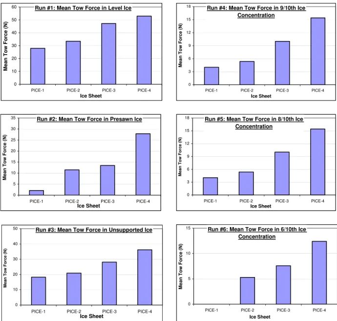
The magnitudes of the (Mean_TFMean) as a function of the model speed and as a
function of the test run # are given in Figures 19a and 19b, respectively. Similarly, the
magnitudes of the (Mean_TFMax) as a function of the model speed and as a function of
the test run # are given in Figures 20a and 20b, respectively. The overall trends seem reasonable, and the same conclusions as those given in Phase I report (Derradji-Aouat, 2002) are reached.
It is important to note that the above procedure (segmentation of measured time history, correction for ice thickness, the use of the three calculation steps) is valid for calculating random uncertainties in all other measured ship motion parameters (pitch, heave, yaw and sway).
11.1 Random Uncertainties in Mean Tow Force
Figures 21a and 21b show the calculated random uncertainties in mean resistance
(Mean_TFMean) as a function of test run type (in Fig. 21a) and as a function of ice sheet
number (in Fig. 21b). The main results are:
• In level (continuous, unbroken) ice test runs (Run # 1, # 2 and # 3), Figs. 21a and 20b and Table 7 show that, the calculated random uncertainties in mean tow forces are less than 6%. In fact, all uncertainties were below 4%, except for two data points (PICE-1, Run # 2 and PICE-4, Run # 3), where uncertainties were 5.84% and 4.08%, respectively.
• In broken ice test runs (Run # 4, # 5 and # 6), Fig. 21a, 21b and Table 7 show that all random uncertainties were below 18%, except for test run # 5 in PICE-1, where the uncertainty value was 25.94 %. It should be emphasized that in broken ice tests, no corrections for ice thickness profiles were made.
11.2 Random Uncertainties in Maximum Tow Force
Calculations of uncertainties in maximum tow force are given in Table 8 (same calculation procedure as for the uncertainties in mean tow force in Table 7). Figures 22a
and 22b show plots for the calculated uncertainties in maximum tow force (Mean_TFMax)
as a function of test run # (Fig. 22a) and as a function of the model speed (Fig. 22b). The main results are:
• In continuous (unbroken) ice test runs (Run # 1, # 2 and # 3), Figs. 22a and 22b and Table 8 show that, all calculated random uncertainties are less than 14%. In fact, all uncertainties were below 10%, except for three data points (PICE-2-Run # 1, PICE-3-Run # 1 and PICE-4-Run # 3), where uncertainties were 10.71%, 13.83% and 11.17 %, respectively.
• In broken ice test runs (Run # 4, # 5 and # 6), Fig. 22a and 22b and Table 8 show that all random uncertainties were below 14 %. It should be re-emphasized that in broken ice tests, no corrections for ice thickness profiles were made.
11.3 Effect of Correction for Ice Thickness on Random Uncertainties
Corrections for variations in ice thickness profiles (using Eq. 4b) are made only for tests in continuous ice (Runs # 1, # 2 and # 3). Figure 23a shows comparisons between corrected versus uncorrected random uncertainties in mean tow force. It is clear that the change in ice thickness did affect much the values of U(TFMean). This is a
different conclusion than those reached in the previous two phases of testing. 11.4 Effects of Data Reduction Equation
Equation 4b was proposed to correct for effects of ice thickness variations on the values of random uncertainties. It should be recognized that the corrected resistance curves are not direct laboratory measurements, but they are calculated from the analytical equation (Eq. 4b). The process of using analytical equations to correct measured parameters is called “Application of Data Reduction Equations, DRE”.
In EUA, there are additional random uncertainties involved in the application of the DRE. The uncertainty involved in using Eq. 4b is:
h U R UR R UR 2 1 2 2 0 h 0 0 ⎟ ⎟ ⎠ ⎞ ⎜ ⎜ ⎝ ⎛ ⎟ ⎠ ⎞ ⎜ ⎝ ⎛ + ⎟ ⎠ ⎞ ⎜ ⎝ ⎛ = ⎟ ⎠ ⎞ ⎜ ⎝ ⎛ (8)
In the above equation, (UR/R) is the total uncertainty in resistance, R. Both
(UR0/R0) and (Uh/h0) are the relative uncertainty in the measured ice resistance (as
calculated in Tables 7 and 8) and the relative uncertainty in the measured ice thickness, respectively (the uncertainties in ice thickness are shown in Table 4). Note that, in Eq. 8, the value of (Uh/h0) is an additional relative uncertainty, which is induced by the use and application of the DRE. The total relative uncertainty is the geometric sum of both
relative uncertainties (UR0/R0) and (Uh/h0).
Tables 9a and 10a give the values for mean and maximum tow forces (mean of the means and means of maximums), respectively. Tables 9b and 10b show the calculated uncertainties in mean and in maximum tow forces before the use of the data reduction
equation. Tables 9c and 10c show the calculated uncertainties in mean and in maximum tow forces after including the additional uncertainty due to the use of DRE.
After adding the effect of the DRE, in mean tow force, all final uncertainties were below 18%, except for test Run # 5 in PICE-1, where the uncertainty value was 25.94 %. In maximum tow force, all calculated random uncertainties are less than 15%.
Application of the DRE does not affect the uncertainties in broken ice test runs. No ice thickness corrections were applied to the results from broken ice tests.
11.5 Comparison of Uncertainties in Continuous Ice and in Broken Ice
In continuous ice (including presawn ice sheets), random uncertainties were mainly under 10%. This is valid for both maximum and mean resistance measurements.
However, in broken ice tests, uncertainties of less than 14% were obtained (except in 2 cases). The value of 14% is higher than the magnitude of uncertainty in continuous ice (10%). The difference between uncertainties in continuous ice and those in broken ice are attributed to several factors (the details were given by Derradji-Aouat, 2002).
11.6 Comparison of Uncertainties in Mean and Maximum Tow Forces
Figures 24a and 24b show comparisons between random uncertainties in mean tow forces and those in maximum tow forces as a function of the test run number (Fig. 24a) and as a function of the model speed (through the ice sheet # in Fig. 24b).
In continuous ice tests, random uncertainties in maximum tow forces are higher than those in mean tow forces (ratio of up to 5:1 for PICE-3, Run # 1). However, no conclusion has been reached in broken ice tests, random uncertainties in mean tow force are both higher and lower than those in maximum tow forces.
12.
Bias and Total Uncertainties
In ice tank testing bias uncertainties are neglected (Derradji-Aouat, 2002), and therefore, the total uncertainties are taken as equal to the random ones.
13.
Comparison of Phase I and III Uncertainties
Tables 11 and 12 present the mean and maximum tow force uncertainties calculated from the results of Phase I and Phase III test programs, respectively. Figures 25a and 25b provide a comparison between uncertainties calculated in Phase I testing and those calculated in Phase III testing. Implicitly, the tables show the effects of the tow post and PMM on random uncertainties. More comparisons between the analyses of test results in Phase I and those in Phase III are provided in Appendix 7.
The main conclusions drawn from the comparisons in Tables 11 and 12 are:
13.1 Uncertainties in Mean Resistance
• In level (continuous, unbroken) ice test runs (Run # 1, # 2 and # 3), the calculated random uncertainties are less than 10% (Table 11). The values for uncertainties in mean tow force in Phase I are generally larger than those of Phase III (Figure 25a).
• In broken ice test runs (Run # 4, # 5 and # 6), all random uncertainties were below 20%, except for Run # 5 in sheet # 1 of Phase III where the uncertainty was 25.94%. The equivalent test in Phase I also experienced the highest uncertainty for that phase at 19.97%.
13.2 Uncertainties in Maximum Resistance
• In the continuous (unbroken) ice test runs (Run # 1, # 2 and # 3) for both phases, all calculated random uncertainties are less than 15% (Table 12), except for one data point at 15.98% (Run # 2 in ice sheet # 4 from Phase I). • In broken ice test runs (Run # 4, # 5 and # 6), all random uncertainties were
below 15 %, except for one data point at 16% (run #5 in ice sheet #2 from Phase I).
14.
Summary, Conclusions and Recommendations
• In continuous ice test runs, the uncertainty range of 3% to 10% was obtained. This is consistent with the range of uncertainties obtained in Phases I and II test programs. The range is also consistent with the previously reported studies (in the literature) using different ship models, in different ice tanks, in different countries over a time span of 10 to 12 years (Derradji-Aouat, 2002).
• In broken ice, the uncertainties ranged from to 3% to 26%. This is also consistent with the calculated range obtained in Phases I and II test programs. The large uncertainties are possible (and sometimes expected) in randomly broken ice.
15. References
ASME PTC 19.1-1998. Test Uncertainty. Supplement to Performance Test Code, Instruments and Apparatus.
Coleman H.W. and Steele W.G. (1998). Experimentation and Uncertainty Analysis for Engineers. John Wiley & Sons publications, 2nd edition, New York, NY, 1998.
Derradji-Aouat A., Moores C. and Stuckless S. (2002). Terry Fox Resistance Tests. The ITTC Experimental Uncertainty Analysis Initiative. IMD report # TR-2002-01.
Derradji-Aouat A. (2002). Experimental uncertainty analysis for ice tank ship resistance experiments. IMD/NRC report # TR-2002-04.
Derradji-Aouat A. and Julien Coëffé. (2003). Terry Fox Resistance Tests – Phase II. The ITTC Experimental Uncertainty Analysis Initiative. IMD report # TR-2003-07.
Derradji-Aouat A. (2003). Phase II Experimental uncertainty analysis for ice tank ship resistance experiments. IMD/NRC report # TR-2003-09.
Derradji-Aouat A. (2004). A Method for Calculations of Uncertainty in Ice Tank Ship Resistance Testing. Proceedings of the 19th International Symposium on Sea Ice, Mombetsu, Japan (Feb. 2004).
GUM (2002): General Uncertainty Measurements (http://www.gum.dk/)
ISO (1995): Guide to the Expression of Uncertainty in Measurements. ISBN 92-67-10188-9.
Marineering Limited (1997). The Development and Commissioning of a Large Amplitude Planar Motion Mechanism. Volume 1: Main Report. IMD/NRC report # CR-1997-05 (Vol.1 of 3).
Table 1: Percentage Difference in Phase I and Phase Mean Tow Forces.
0.1 34.54 27.77 21.73% 0.2 46.00 33.45 31.59% 0.4 56.49 46.47 19.46% 0.6 63.96 52.07 20.49% 0.1 11.58 2.11 138.35% 0.2 13.18 11.24 15.92% 0.4 20.50 13.41 41.83% 0.6 29.76 27.80 6.82% 0.1 25.11 18.01 32.96% 0.2 34.65 20.76 50.15% 0.4 44.30 27.71 46.06% 0.6 52.22 35.44 38.28% 0.1 7.06 5.67 21.85% 0.2 8.99 8.49 5.75% 0.4 14.50 12.24 16.87% 0.6 20.14 17.78 12.45% 0.1 5.11 4.04 23.50% 0.2 7.58 5.37 34.11% 0.4 9.50 10.02 5.38% 0.6 16.41 15.43 6.14% 0.1 2.21 n/a n/a 0.2 4.71 5.29 11.67% 0.4 9.23 7.59 19.49% 0.6 13.23 12.41 6.38% Phase 1: Tow Post Phase 3: PMM 1 2 3 4 5 6 Speed (m/s) % Difference Run #
Note: The shaded data points are outliers.
Table 2: Percentage Difference in Phase I and Phase III Maximum Tow Force.
0.1 67.7 79.95 16.59% 0.2 121.34 144.78 17.62% 0.4 203.66 321.75 44.95% 0.6 261.71 433.82 49.49% 0.1 45.1 21.55 70.67% 0.2 45.48 34.82 26.55% 0.4 53.55 60.61 12.37% 0.6 65.91 94.71 35.86% 0.1 54.47 63.42 15.18% 0.2 93.96 65.26 36.05% 0.4 154.22 219.12 34.77% 0.6 242.18 358.09 38.62% 0.1 37.48 25.51 38.00% 0.2 30.78 29.20 5.28% 0.4 39.39 45.62 14.65% 0.6 50.87 85.78 51.09% 0.1 21.03 20.66 1.79% 0.2 20.52 21.02 2.42% 0.4 25.89 32.85 23.70% 0.6 36.2 56.04 43.01% 0.1 36.37 n/a n/a 0.2 25.13 19.78 23.81% 0.4 27.99 31.37 11.40% 0.6 33.88 51.92 42.06% 6 1 2 3 5 % Difference Phase 1: Tow Post Phase 3: PMM Run # Speed (m/s) 4
Table 3a: Slope for tow force time histories.
Run # 1: Run # 2: Run # 3: Run # 4: Run # 5: Run # 6:
Level Ice Pre-sawn Unsupported 9/10th 8/10th 6/10th
PICE-1 0.50% 0.11% 1.00% 0.28% 0.92% n/a
PICE-2 1.57% 0.03% 0.002% 0.67% 1.40% 0.76%
PICE-3 1.09% 0.14% 1.38% 0.74% 0.91% 1.58%
PICE-4 5.19% 1.31% 1.22% 1.75% 1.89% 2.27%
Ice Sheet
Continuous Ice Tests Broken Ice Tests
Table 3b: Change in measured tow force during the long test runs (~65m).
Run # 1: Run # 2: Run # 3: Run # 4: Run # 5: Run # 6:
Level Ice Pre-sawn Unsupported 9/10th 8/10th 6/10th
PICE-1 9.66% 27.16% 2.87% 23.87% 121.57% n/a
PICE-2 12.03% 0.73% 0.026% 21.40% 68.72% 40.63%
PICE-3 3.03% 1.35% 6.19% 7.98% 12.10% 28.47%
PICE-4 8.77% 4.24% 2.91% 8.50% 10.80% 15.76%
Ice Sheet
Continuous Ice Tests Broken Ice Tests
Table 3c: Slope for carriage speed time histories.
Run # 1: Run # 2: Run # 3: Run # 4: Run # 5: Run # 6:
Level Ice Pre-sawn Unsupported 9/10th 8/10th 6/10th
PICE-1 1.E-06 1.E-06 8.E-07 1.E-06 1.E-06 n/a
PICE-2 2.E-06 2.E-06 2.E-06 2.E-06 8.E-07 4.E-07
PICE-3 5.E-07 2.E-07 8.E-07 1.E-07 1.E-08 4.E-06
PICE-4 2.E-06 6.E-07 6.E-06 3.E-06 2.E-06 3.E-06
Ice Sheet
Continuous Ice Tests Broken Ice Tests
Table 3d: Change in measured carriage speed during the long test runs (~65m).
Run # 1: Run # 2: Run # 3: Run # 4: Run # 5: Run # 6:
Level Ice Pre-sawn Unsupported 9/10th 8/10th 6/10th
PICE-1 0.53% 0.50% 0.41% 0.48% 0.52% n/a
PICE-2 0.26% 0.27% 0.27% 0.27% 0.11% 0.055%
PICE-3 0.016% 0.006% 0.025% 0.003% 0.0003% 0.14%
PICE-4 0.029% 0.009% 0.085% 0.043% 0.030% 0.044%
Ice Sheet
Table 4: Experimental Uncertainty Calculations for Ice Sheet Thickness Profiles. Thickness (mm)
Tank Position
(m) PICE-1 PICE-2 PICE-3 PICE-4
0 38.5 2 38.35 37.58333 38.51667 38.18333 4 38.66667 38.21667 38.6 38.4 6 39.08333 39.01667 39.23333 38.6 8 39.65 39.7 40 38.95 10 39.98333 39.88333 40.36667 39.08333 12 39.98333 39.66667 39.86667 39.2 14 39.76667 39.1 39.55 39.1 16 39.73333 39.06667 39.36667 39.2 18 39.91667 39.93333 39.5 38.68333 20 40.46667 40.05 39.93333 39.38333 22 40.18333 39.23333 39.75 39.63333 24 39.86667 38.98333 39.35 39.48333 26 39.43333 38.81667 39.26667 39.05 28 39.18333 38.93333 39.38333 39.05 30 39.53333 38.61667 39.26667 38.95 32 39.61667 38.23333 39.11667 38.75 34 39.56667 38.3 38.81667 38.71667 36 39.75 38.98333 39.23333 39.23333 38 40.3 39.21667 39.6 39.81667 40 40.01667 38.76667 39.48333 39.8 42 39.6 38.25 38.85 39.23333 44 39.23333 38 38.3 38.75 46 39.3 38.18333 38.55 38.56667 48 39.61667 38.36667 38.66667 38.8 50 39.95 39.28333 38.9 39.31667 52 40.55 40.33333 39.2 40.05 54 40.53333 40.31667 39.46667 40.65 56 40.08333 39.21667 39.36667 40.16667 58 39.7 38.63333 38.8 39.45 60 39.68333 38.66667 38.76667 39.38333 62 40 38.5 39.38333 39.63333 64 38.86667 39.25 40 66 38.25 H mean 39.72419 38.94444 39.2043 39.18118 STDEV 0.479561 0.684332 0.434549 0.530259 Uh(N) 0.959121 1.368664 0.869098 1.060518 Uh(%) 2.41% 3.51% 2.22% 2.71%
Table 5a: Ice Flexural Strength Components (measured values and experimental uncertainty calculations). 0.2030 0.0885 0.0396 2.79 0.2000 0.0851 0.0387 2.60 0.1960 0.0835 0.0397 2.70 0.2050 0.0815 0.0388 2.60 0.2010 0.0869 0.0394 2.60 0.2100 0.0795 0.0387 2.89 0.2050 0.0976 0.0388 3.68 0.2100 0.0854 0.0385 2.53 0.1950 0.1080 0.0399 3.53 0.1950 0.0834 0.0387 2.01 0.2000 0.1000 0.0405 3.58 0.2050 0.0822 0.0389 1.96 0.2080 0.0930 0.0390 2.79 0.1950 0.0937 0.0385 2.30 0.1970 0.0842 0.0390 2.50 0.1920 0.0931 0.0387 2.06 0.1950 0.0869 0.0393 2.79 0.1850 0.0770 0.0385 2.11 0.2080 0.0843 0.0394 2.94 0.1950 0.0761 0.0390 2.06 0.2150 0.0845 0.0391 2.60 0.1950 0.0808 0.0389 2.26 0.2050 0.0812 0.0392 2.84 0.1900 0.0850 0.0386 2.65 0.1500 0.0852 0.0405 1.47 0.1250 0.0820 0.0392 1.23 0.2050 0.0848 0.0407 1.72 0.1880 0.0815 0.0398 1.18 0.2050 0.0850 0.0414 1.96 0.2100 0.0865 0.0393 1.18 0.1950 0.0839 0.0411 1.37 0.2000 0.0826 0.0395 1.18 0.2000 0.0822 0.0409 1.37 0.2000 0.0805 0.0407 1.03 0.2000 0.0834 0.0405 1.47 0.1800 0.0835 0.0400 1.03 0.2000 0.0755 0.0405 0.98 0.2000 0.0786 0.0405 0.83 0.1850 0.0794 0.0414 1.03 0.2080 0.0771 0.0397 1.18 0.1940 0.0893 0.0404 2.45 0.1920 0.0881 0.0387 1.86 0.1980 0.0841 0.0405 2.40 0.2080 0.0870 0.0388 1.91 0.1850 0.0829 0.0404 2.35 0.2050 0.0893 0.0391 2.21 0.2080 0.0867 0.0405 2.45 0.1900 0.0865 0.0387 2.11 0.2000 0.0874 0.0406 2.50 0.1850 0.0835 0.0400 2.06 0.2100 0.0746 0.0406 1.47 0.2000 0.0797 0.0395 1.86 0.2000 0.0865 0.0405 2.70 0.1950 0.0830 0.0397 1.96 0.2000 0.0865 0.0405 2.70 0.1600 0.0827 0.0393 2.65 0.2000 0.0879 0.0403 3.92 0.2050 0.0837 0.0382 2.84 0.2120 0.0898 0.0395 3.04 0.2050 0.0832 0.0389 2.72 0.1980 0.0845 0.0396 2.94 0.2050 0.0781 0.0389 3.04 0.2050 0.0842 0.0393 3.38 0.2100 0.0815 0.0399 3.19 0.2000 0.0811 0.0389 3.48 0.2100 0.0883 0.0399 3.09 0.2050 0.0799 0.0399 1.72 0.1900 0.0828 0.0383 2.79 Mean 0.201 0.0853152 0.0400412 2.4767647 0.1900 0.0846 0.0395 3.14 STDEV 0.0065717 0.0051048 0.0007382 0.7841796 0.2000 0.0866 0.0385 2.06 U (%) 6.54% 11.97% 3.69% 63.32% 0.2000 0.0815 0.0390 2.75 0.2000 0.0827 0.0385 2.89 0.1920 0.0826 0.0385 2.84 0.1900 0.0849 0.0381 2.75 0.1950 0.0846 0.0379 3.04 0.2000 0.0832 0.0383 3.14 Mean 0.19825 0.08291 0.0389927 2.232619 STDEV 0.0079928 0.0031143 0.0006006 0.6812258 U (%) 8.06% 7.51% 3.08% 61.02% 15N PICE-2
Location Length (m) Width (m) Thickness
(m) Load (N) 60N 31S 38N 38S 39N 39S PICE-1
Location Length (m) Width (m) Thickness
(m) Load (N) 15N 15S 31N 39N 39S 40N 15S 30N 30S 38N 60N 60S 38S 60S 40S