HAL Id: hal-00345968
https://hal.archives-ouvertes.fr/hal-00345968
Submitted on 10 Dec 2008
HAL is a multi-disciplinary open access
archive for the deposit and dissemination of
sci-entific research documents, whether they are
pub-lished or not. The documents may come from
teaching and research institutions in France or
abroad, or from public or private research centers.
L’archive ouverte pluridisciplinaire HAL, est
destinée au dépôt et à la diffusion de documents
scientifiques de niveau recherche, publiés ou non,
émanant des établissements d’enseignement et de
recherche français ou étrangers, des laboratoires
publics ou privés.
FAST: acceleration from theory to practice
Sebastien Bardin, Alain Finkel, Jérôme Leroux, Laure Petrucci
To cite this version:
Sebastien Bardin, Alain Finkel, Jérôme Leroux, Laure Petrucci. FAST: acceleration from theory to
practice. International Journal on Software Tools for Technology Transfer, Springer Verlag, 2008, 10
(5), pp.401-424. �10.1007/s10009-008-0064-3�. �hal-00345968�
(will be inserted by the editor)
FAST: Acceleration from theory to practice
⋆
S´ebastien Bardin1, Alain Finkel2, J´erˆome Leroux3, Laure Petrucci4
1
LSL (LIST, CEA), Saclay
e-mail: [email protected] 2
LSV (UMR CNRS 8643, ENS de Cachan), Cachan e-mail: [email protected]
3
LaBRI (UMR CNRS 5800, ENSEIRB, Universit´e Bordeaux-1), Bordeaux e-mail: [email protected]
4
LIPN (UMR CNRS 7030, Universit´e Paris-13), Villetaneuse e-mail: [email protected]
The date of receipt and acceptance will be inserted by the editor
Abstract. Fast is a tool for the analysis of systems ma-nipulating unbounded integer variables. We check safety properties by computing the reachability set of the sys-tem under study. Even if this reachability set is not nec-essarily recursive, we use innovative techniques, namely symbolic representation, acceleration and circuit selec-tion, to increase convergence. Fast has proved to per-form very well on case studies. This paper describes the tool, from the underlying theory to the architecture choices. Finally, Fast capabilities are compared with those of other tools. A range of case studies from the literature is investigated.
Keywords: counter systems, infinite reachability set, symbolic representation, acceleration
1 Introduction
Automatic verification of reactive systems is a major field of research. A popular way of modeling such sys-tems is by means of concurrent automata with shared variables. The automata represent the control structure of the system, while variables encode data. Many classes of such extended automata have been studied, consider-ing variables rangconsider-ing over integers (counters), real num-bers (time), words (queues, stacks) and so on.
The semantics of such an extended automaton is given by a transition system (C, −→), defined by a set of config-urations C and a transition relation −→. A configuration c ∈ C is a tuple of control locations (one for each com-ponent) and a valuation for each variable of the system.
⋆
This paper is mainly based on results presented at CAV 2003, TACAS 2004 and ATVA 2005.
The transition relation −→ is a binary relation over the set of configurations. A configuration c′is reachable from
a configuration c if and only if (c, c′) ∈−→∗, where −→∗
de-notes the reflexive and transitive closure of −→. The set of configurations reachable from the configuration c0 is
called the reachability set from c0.
Safety properties are expressed in terms of “safe reach-able configurations”. They are the most commonly en-countered properties in practice, and allow specification of important properties such as the absence of deadlock, capacity overflow and division by zero.
The class of counter systems, where variables range over integers, appears to be interesting. From a practi-cal point of view, these systems allow the modeling of, for example, communication protocols [18], multi-thread programs or programs with pointers [8]. From a theoret-ical view, many well-known classes appear to be encom-passed by counter systems, like Minsky machines, Petri nets extended with reset/ inhibitor/ transfer arcs [32, 39], reversal-bounded counter machines [47] and broad-cast protocols [33,34].
The counterpart of the expressiveness of counter sys-tems is that only two counters with increment, decre-ment and test-to-zero can simulate a Turing machine. Then checking even basic safety properties of counter systems is undecidable. Many works have been conducted on identifying decidable subclasses, like Petri nets [60] and reversal-bounded counter machines [46,47]. How-ever few of these results have been implemented, mainly for two reasons. First since each result applies for a re-stricted subclass, there is no generic method for a large class of counter systems. Second, these algorithms are often inefficient in practice.
1.1 The tool Fast
In this paper, we present the tool Fast [5,9], designed to check safety properties on counter systems. We made the choice to consider a very large subclass of counter sys-tems, namely linear counter syssys-tems, for which checking safety properties is undecidable.
The safety properties are expressed in terms of Pres-burger constraints over counters. They strictly include the usual reachability properties, expressed in terms of control location or upward closed / convex sets of con-figurations.
The tool Fast has four main advantages:
Since linear counter systems and Presburger constraints are very expressive, Fast can be applied to a large spectrum of applications and the tool is not tied to a particular specific case-study.
Despite the inherent theoretical limitations, a powerful engine based on recently developed techniques (accel-eration, flattening, reduction) allows Fast to check the correctness of the system in most practical cases. Fast design is fully based on a clear theoretical frame-work (flat acceleration). Abilities and limits of the tool are clearly identified: Fast is complete for the class of flattable systems [7]. Moreover since many decidable subclasses of counter systems are flattable, Fastprovides a unified verification algorithm for all these classes [56,57].
Finally, in case the automatic verification fails, the user can guide the tool using a script language. We think that this is an important feature since termination cannot be guaranteed.
1.2 Theoretical foundations
Symbolic model checking. Fast follows the model check-ing approach [13,26], based on the exhaustive explo-ration of the reachability set. However, since one manip-ulates potentially infinite sets of configurations, called regions, the model checking must be “symbolic”. A sym-bolic representation must support the following opera-tions: (1) post- and/or pre-image computation, (2) union to collect all reachable configurations, (3) inclusion to test for fixpoint. The most popular symbolic represen-tations are based on regular languages: these are quite expressive and automata-theoretical data structures pro-vide well-known and efficient algorithms performing the previous operations. With these ingredients, it becomes possible to launch a fixpoint computation for forward or backward reachability sets (see for example [51]), as exemplified in procedure 1.
Acceleration. In practice, an iterative symbolic reacha-bility set computation similar to the one of procedure 1 will surely fail. A solution to help convergence is to use
procedure reach1(x0)
input: symbolic configuration x0.
1: x ← x0
2: while post(x) 6⊑ x do
3: x ← post(x) ⊔ x
4: end while
5: return x
Procedure 1: standard symbolic procedure acceleration techniques. Acceleration consists of comput-ing in one step the effect of the transitive closure of a transition or a sequence of transitions.
First ideas of acceleration can be found in the cover-ing tree of Petri nets by Karp and Miller in 1969 [49], extended by Finkel to well-structured transitions sys-tems [36]. The first paper on the acceleration of counter systems is probably due to Boigelot and Wolper in [21], considering functions with increment/ decrement/ reset and convex guards. Since then, lots of work has been achieved in this area, for example [2,14,41,42,50]. Re-sults of [20,37,66] extend those of Wolper and Boigelot to linear functions with Presburger-definable guards. Flat acceleration framework. An efficient acceleration algorithm is not sufficient to compute the reachability set. The question is how to find out the circuits (se-quences of transitions) of the system, whose acceleration will lead to a successful computation of the reachability set. This issue was not clearly treated until we intro-duced the flat acceleration framework [7]. We proposed the notion of flattening, and showed that flat acceler-ation computes the reachability set if and only if the system is flattable. Moreover, we designed a complete heuristic for flattable systems, and generic optimizations called reductions. The framework is articulated around four key points: (1) the system under consideration, (2) the symbolic representation, (3) the acceleration algo-rithm and (4) a heuristic to select circuits to be acceler-ated.
The tool Fast follows strictly the flat acceleration framework. The systems analyzed (linear counter sys-tems with finite monoid) and the corresponding accel-eration algorithms can be found in [37,66]. The sym-bolic representation is based upon the automata repre-sentation of semi-linear sets (see [23,67]). The selection heuristic is the one described in [7] with the reduction presented in [37].
Even though the reachability set of a linear counter system is not Presburger definable in general, in prac-tice the systems manipulated are regular enough to have a Presburger definable reachability set. The techniques presented throughout the paper allow for model checking many counter systems (more than forty tests).
Moreover, Leroux and Sutre have shown in [56,57] that Fast is guaranteed to terminate for many
sub-classes of counter systems: 2-counters VASS, reversal-bounded counter machines, lossy VASS, BPP, Cyclic Petri nets and other subclasses.
1.3 Other tools for counter systems
The following approaches and tools have been developed to check correctness of counter systems.
Reachability set computation. Tools Alv [25,68], Lash [55] and TReX [3] implement symbolic methods to compute the forward reachability set of counter systems. Alv pro-vides two different symbolic representations for integer vectors: Presburger formula or automata as in Fast. Ac-celeration is available for the formula-based representa-tion [50], but not for the automata-based representarepresenta-tion. The tool is mostly used in backward computation or in approximated forward computation [12]. Lash [55] foun-dations are close to those of Fast, with similar symbolic representations and acceleration algorithms. The main difference is that Lash does not implement any circuit search and the user has to provide circuits to the tool. TReX [3] follows the same framework but uses rather different technologies. A comparison of Alv, Fast, Lash and TReX is presented in section 8.
Co-reachability set computation. One of the most inter-esting results for counter systems verification is the com-putability of the co-reachability set of monotonic VASS: monotonic VASS is a large subclass, efficient symbolic representations have been developed and interesting case studies have been conducted. We can cite the work on covering sharing trees of Delzanno, Raskin and Van Be-gin [30] and the tool brain by Voronkov and Rybina [64]. These approaches are more specific than the one of Fast: computation is backward only1, properties are reduced
to upward-closed sets and systems are monotonic. For example case-studies of section 9 and section 10 could not have been handled with these tools.
Reachability set approximation. Finally, some approaches relax the exactness of computation to ensure computa-tion terminacomputa-tion or at least simpler computacomputa-tional steps. However the superset obtained in the end may not be tight enough to decide the property. We can cite the classic tool Hytech [1], as well as the abstract-check and refine technique of Raskin et al. [44] to compute iteratively covering trees of monotonic Petri nets. 1.4 Contribution
This paper provides both an overview of the main re-sults obtained on Fast and on acceleration of counter systems [4,5,7,9,10,29,37,56,57] as well as some origi-nal contributions: an up-to-date description of Fast, an
1 Fast
can also be used for backward reachability computations.
in-depth experimental comparison with similar tools, the verification of the TTP protocol (a short description of this work was proposed in [4]) and the verification of the Capacity Exchange Signaling protocol.
1.5 Outline
The sequel of the paper is structured as follows. Each point of the Fast framework is presented in sections 2 to 5: counter systems (section 2), symbolic representa-tion (secrepresenta-tion 3), accelerarepresenta-tion (secrepresenta-tion 4) and selecrepresenta-tion heuristic (section 5). After this overview of the theoret-ical foundations, section 6 presents the tool Fast. Ex-periments are presented in section 7, comparisons with tools Alv, Lash and TReX can be found in section 8 and two case-studies are developed in sections 9 and 10.
2 Presburger Arithmetic And Counter Systems 2.1 Sets
Given two sets E and F , we denote by E ∪F , E ∩F , E\F and E ×F , the union, the intersection, the difference and the Cartesian product of E and F . The set Ei, i >0, is
defined by E1= E and En+1= E×En. We write E ⊆ F
if E is a subset of F . The empty set is denoted ∅. Given two sets E, X such that E ⊆ X, the complement of E (in X) is denoted by ¯Eand is defined as ¯E= X\E. The cardinal of a finite set X is written |X|.
2.2 Relations
A relation R between E and F is a subset R ⊆ E × F. We write x R x′ whenever (x, x′) ∈ R. The inverse
relation of R, written R−1⊆ F ×E, is defined by x′R−1x
if and only if xRx′. The image of x ∈ E by R is the
set R(x) ⊆ F defined by R(x) = {x′ ∈ F |xRx′}. The
definition is extended to a set X ⊆ E by R(X) = {x′∈
F|∃x ∈ X.xRx′}. Given two relations R
1 ⊆ E × F and
R2 ⊆ F × G, the composition of R1 and R2, written
R1• R2 ⊆ E × G, is defined by: x(R1• R2)x′′ if xR1x′
and x′R
2x′′ for some x′ ∈ F .
A binary relation R on E is a relation between E and itself. The identity relation on E is the binary relation IdE = {(x, x)| x ∈ E}. For R on E, we denote by Ri
the relation defined inductively by: R0 is the identity
relation on E and Rn+1 = R • Rn. The reflexive and
transitive closure of R, denoted R∗, is then defined by
R∗=S
n≥0Rn.
2.3 Numbers and matrices of numbers
Let Z (resp. N) denote the set of integers (resp. non-negative integers). We denote by Mn(Z) (resp. Mn(N))
q1 q2 x′= x + 1 ∧ y′= y /∗ a1 ∗/ x 6= y ∧ y′= y + x ∧ x′= x /∗ a2 ∗/ y′= y + 2∧ x′= x − 1 /∗ a3∗/
Fig. 1: A simple counter system
the set of square matrices of size n over Z (resp. N). The identity matrix of size n is denoted 1n. The max-norm
of a matrix (resp. vector), written ||·||∞, is the maximal
absolute value appearing in the matrix (resp. vector). 2.4 Presburger arithmetic
Presburger arithmetic [63] is the first order additive the-ory over the integers hZ, ≤, +i. Satisfiability and valid-ity of Presburger arithmetic are both decidable. A Pres-burger formula is denoted by φ(−→x) where −→x is a n-dim vector of free variables (−→x[i] is the i-th component of −→x). The set of vectors defined by such a formula φ(−→x), i.e, the set of vectors satisfying φ, is denoted by q
φ(−→x)y⊆ Zn. A set X ⊆ Zn is said to be
Presburger-definable if there exists a Presburger formula φ(−→x) such that X =qφ(−→x)y.
2.5 Counter systems
A counter system is a finite control structure (automa-ton2) extended with m integer variables whose values
can be modified by actions denoted by a Presburger for-mula. Fig. 1 gives an example of a counter system. Definition 1 (Counter system). Let m be a non-negative integer. A m-dim counter system S is a tuple S= (Q, T, m), where Q is a finite non empty set of loca-tions, and T is a finite set of transitions (q, φ, q′) where
q, q′ ∈ Q and φ(−→x , −→x′) is a Presburger formula over 2m variables.
Given a transition t = (q, φ, q′) ∈ T , we define the
functions α, β and l by α(t) = q, β(t) = q′ and l(t) = φ.
Semantics. As previously mentioned, the semantics of a counter system is given by a transition system (CS,
T
−→). The set of configurations CS of a counter system S is
Q× Zm. The transition relation−→ is defined as follows.T
The semantics of a transition t ∈ T is given by the re-lation−→ over Ct S defined by: (q, −→x)
t
−→ (q′, −→x′) if q =
α(t), q′ = β(t) and (−→x , −→x′) ∈ Jl(t)K. This definition can
be extended to the set T∗of sequences of transitions. Let
us denote by ε the empty word. Then −→ε def= IdCS and
t·π
−→def=−→ •t −→. We also extend −→ to any languageπ 2
In case of multi-component systems, we consider the synchro-nized product automaton.
L⊆ T∗ by−→L def= S
π∈L π
−→. The definition of −→ fol-T lows directly. The relation−→ is called the reachabilityT∗ relation.
Remark 1. The analysis of a counter system with |Q| locations and m counters can always be reduced to the analysis of a system S′= ({q′}, T′, m+ 1) with only one
location and m + 1 variables, by encoding the control structure in a new counter xQ.
Notation. Whenever S is implicitly known, it is omitted in the notation.
2.6 Reachability problems
For any X ⊆ C and any L ⊆ T∗, the set post(L, X) of
configurations reachable from X following sequences of transitions in L is defined by post(L, X) = (−→)(X) =L {x′∈ C| ∃x ∈ X; (x, x′) ∈ L
−→}. We focus on two partic-ular sets: the set post(T, X) of all configurations reach-able in one step from X, also denoted by post(X); and the set post(T∗, X) of all configurations reachable from
X (the reachability set of X), also denoted by post∗(X).
Given an initial set of configurations X0, checking a
safety property P can be done by: (1) computing post∗(X 0),
(2) deciding whether post∗(X
0) ⊆ P holds or not. We
focus here on the reachability set computation, which is the central issue. Since counter systems generalize Min-sky machines (counters with increment, decrement and test-to-zero), their reachability sets are not recursive in general. Then the best we can hope for are correct proce-dures, with no theoretical guarantee of termination but efficient on large subclasses and practical case-studies.
A symmetrical approach is to compute in a backward manner the co-reachability set pre∗( ¯P) = (−L→)−1( ¯P) and
check that X0∩ pre∗( ¯P) is empty. In the following we
al-ways consider forward computation, but our results can be straightforwardly adapted to backward computation.
3 Automata-Based Symbolic Representation The symbolic model checking approach was first devel-oped to verify large but still finite-state systems. The key idea is to manipulate sets of states directly through a concise symbolic representation (such as BDDs) rather than manipulate enumerations of concrete states. The approach naturally extends to infinite state verification using more complex symbolic representations, such as automata.
In the case of counter systems, the class of Presburger-definable sets is naturally used as the symbolic represen-tation, since: (1) the union of two Presburger-definable sets is effectively Presburger-definable, (2) assuming the
set X is Presburger-definable and S is a counter system, then postS(X) is Presburger-definable, (3) we can check
if X ⊆ X′ for any two Presburger-definable sets X and X′.
3.1 Number Decision Diagrams (ndd)
The efficiency of the algorithms based on Presburger de-finable sets depends strongly on the symbolic represen-tation used for manipulating these sets. Different tech-niques [43] and tools have been developed for manipulat-ing Presburger-definable sets: by workmanipulat-ing directly on the Presburger formulas [52] (implemented in Omega [62]), by using semi-linear sets [45] (implemented in Brain [64]), or by using Number Decision Diagrams [23,65] (ndd, implemented in Fast [5], Lash [55] and Mona [53]).
The ndd representation is obtained by remarking that given a basis r ≥ 2 of decomposition, an integer, or more generally an integer vector in Nm, can be decomposed
into a word over the alphabet Σr,m = {0 . . . r − 1}m.
Then a “regular” set of integer vectors can be
decom-posed into a regular language L ⊆ Σ∗
r,m, and it can
be naturally represented by an automaton over Σr,m.
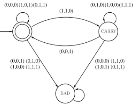
Such an automaton is called a ndd [23,65]. An example is presented in figure 2. For more detailed information on ndd and automata-theoretic representations of Pres-burger sets, the reader is referred to [23,65,67].
(1,1,0) (0,0,1) (1,1,1) (0,1,0) (0,0,0) (1,0,1) (1,1,0) (0,1,1) (0,0,1) (1,0,0) (0,1,0)(1,0,0) (0,1,1) (1,0,1) (0,0,0) (1,1,1) CARRY BAD
Fig. 2: An automaton to represent {(x, y, z)|x + y = z} (least digit first)
This approach is very fruitful since set-theoretical operations correspond to well-known operations on au-tomata (intersection for conjunction, complementation for negation, projection for quantification and so on). Presburger-definable sets and Presburger-definable rela-tions (on 2m variables (−→x , −→x′)) are canonically repre-sented (uniqueness of the minimal form w.r.t. the num-ber of nodes of the ndd). The post- and pre-operations for arbitrary ndd-definable relations are also quite straight-forward, since ndd-definable sets are closed by image of such relations.
Automata representations are well-suited for appli-cations that require a lot of boolean manipulations such as model-checking. For these applications, ndd have two crucial advantages over Presburger formula and semi-linear sets. First, a minimization procedure for automata provides a canonical representation for ndd-definable sets (a set represented by a ndd). This means that the ndd representing a given set only depends on this set and not on the way it is computed. On the other hand, Pres-burger formulas and semi-linear sets lack canonicity. As a direct consequence, a set that possesses a simple rep-resentation could unfortunately be represented in an un-duly complicated way. Second, deciding if a given vector of integers is in a given set can be performed in linear time with ndd, while it is at least NP-hard [15,45] with Presburger formula and semi-linear sets.
Remark 2. In practice, in order to decrease the number of output transitions in the ndd, the basis r is set to 2 (binary decomposition) and the alphabet {0, 1}mis
re-duced to {0, 1} thanks to a serialization [67]. This can be done without any loss of expressivity since Presburger-definable sets are exactly the sets that can be represented by ndd in any basis r of decomposition. People interested in the expressive power of ndd should consult [24].
4 Reachability Computation For Flat Counter Systems
Procedure 1 only terminates on bounded systems [7]: any configuration x ∈ post∗(X) must be reachable from a
configuration x0 ∈ X by a path x0 −→ x where |π| isπ
bounded independently of x and x0. In practice systems
are rarely bounded. For example any linear counter sys-tem (S, X0) such that post∗(X0) is infinite while X0is
fi-nite (e.g. a system with a circuit adding one to a counter) is not bounded. A notable exception is the class of mono-tonic Petri nets, considering backward computation from upward-closed sets of configurations.
Procedure 1 can be improved by using an algorithm post star that computes from a symbolic representa-tion of X and a regular language L ⊆ T∗, a symbolic
rep-resentation of post(L, X). We are interested in infinite regular languages L, simple enough so that post(L, X) can be effectively computed from any set X. Indeed, if Lis finite, then post(L, X) can be computed by proce-dure 1 and post star does not add any power to pro-cedure 1. On the other hand, post(L, X) cannot be com-puted for an arbitrary L, since post(T∗, X) is equal to
the reachability set which is not recursive. In the sequel, we consider the special case L = σ∗ where σ ∈ T∗.
It is easy to define a first syntactic restriction to counter systems such that the reachability set can be computed with an improved version of procedure 1 using post(σ∗, X) for some cycles σ ∈ T∗. We call flat counter
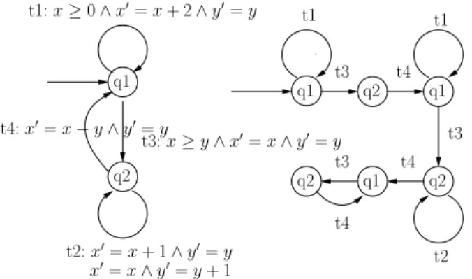
system [27,38,40] a counter system where, for each lo-cation q, there exists at most one elementary circuit in the control graph containing q (see figure 3). Intuitively a flat system has no nested loop. For example, to com-pute the reachability set of the flat counter system of figure 3, we first iterate t1, then fire t3 and finally
it-erate t2. Note that such an algorithm (if it exists) goes
beyond the standard symbolic procedure because it can discover the set of configurations that are not necessarily reachable by paths of a bounded length.
t1: x≥ 0 ∧ x′= x + 2∧ y′= y
t2: x′= x + 1∧ y′= y + 1
t3: x≥ y ∧ x′= x∧ y′= y
q1 q2
Fig. 3: A flat counter system
4.1 Presburger linear functions
The set post(σ∗, X) is not Presburger-definable in
gen-eral even if X is Presburger-definable. Indeed, this set can be non-recursive since the one-step reachability rela-tion R of a Minsky machine is Presburger-definable and can be encoded by a single loop t such that Jl(t)K = R. Nevertheless, we say that a Presburger-definable binary relation R ⊆ Zn× Zn can be accelerated if the binary
relation R∗ is Presburger-definable. In this section, we
define a subclass of Presburger-definable binary relations R, both encompassing most of the usually used binary relations R = Jl(σ)K and supporting the effective com-putation of a Presburger formula encoding R∗.
Definition 2 (Presburger linear function [37]). A Presburger linear function is a function f : Zn → Zn
such that there exists a tuple ¯f = (ϕ, M, −→v), where ϕ(−→x) is a Presburger formula over n variables, M ∈ Mn(Z) is a square matrix and −→v ∈ Zn is a vector, such
that f is defined over JϕK by f(−→x) = M.−→x + −→v. Such a tuple ¯f = (ϕ, M, −→v) is called a Presburger linear presentation of f . The formula ϕ is the guard of ¯f.
Note that the binary relation x′ = f (x) where f is
the Presburger linear function defined by f (x) = 2x for any x is not accelerable. In fact, the binary rela-tion x′ ∈ f∗(x) is not Presburger-definable. We
intro-duce the class of Presburger linear presentations with a finite monoid to enforce the accelerability property. The monoid of a Presburger linear presentation ¯f = (ϕ, M, −→v) is the multiplicative monoid M∗ of the
ma-trix M , i.e. M∗= {1
m, M, M2, . . . , Mn, . . .}.
Note that when M = Idm the Presburger
presenta-tion ¯f = (ϕ, M, −→v) has a finite monoid. In this case, the
binary relation−→x′ ∈ f∗(−→x) is encoded by the following
Presburger formula:
∃k ≥ 0, −→x′ = −→x + k−→v ∧ ∀0 ≤ l < k, ϕ(−→x + l−→v) (1) In fact, the following theorem holds.
Theorem 1 ([20, 37]). The binary relation f∗ is
ef-fectively Presburger-definable for any Presburger linear presentation ¯f with a finite monoid.
Proof. (Sketch) We reduce the proof to the straightfor-ward case M = Idm. As ¯f = (ϕ, M, −→v) has a finite
monoid, there exists an integer n ≥ 0 and an integer p ≥ 1 such that Mn+p = Mn. For any integer k ≥ 0
we denote by (ϕk, Mk, −→vk) a presentation of fk. Let us
consider the Presburger linear function g defined by the presentation ¯g = (fn(ϕ
n+p), Idm,(Mp− Idm)−→vn+ −→vp).
We observe that fp+n= g ◦fnand the following equality
provides the reduction: f∗= n−1 [ r=0 fr p−1 [ r=0 g∗◦ fn+r ⊓ ⊔
Remark 3. The finiteness of the monoid of a Presburger linear presentation is decidable in polynomial time [19]. We have proved that for a Presburger linear presenta-tion ¯f = (ϕ, M, −→v) with a finite monoid, the transition relation f∗ can be expressed as a Presburger formula.
Then computing a ndd representing f∗ can be achieved.
An upper bound for the construction of this ndd is 3-EXPTIME in the size of the ndd encoding ϕ (denoted |A(ϕ)|), the values
−→v
∞and ||M ||∞, and the number
of counters m. The algorithm is implemented in Fast and the upper bound has never been reached on case-studies, except for the TTP system (with two faults), for which we have designed a special acceleration algo-rithm that takes into account the particular form of the functions f manipulated.
For some subclasses of Presburger linear functions f with a finite monoid, a more efficient algorithm for computing f∗can be expected.
Definition 3 (Convex translation [4]). A convex trans-lation f is a Presburger linear function f = (ϕ, 1m, −→v)
where 1mis the identity matrix and ϕ is a convex
poly-hedron.
Convex translations are a subclass of Presburger lin-ear functions with finite monoid. The class encompasses for example Petri nets and Minsky machines. Actually, we can use geometrical properties of convex sets to alle-viate the transitive closure construction. In fact, in this case the Presburger formula (1) can be replaced by the following one:
parameter (magnitude) standard algo. convex algo. |A(ϕ)| (105 ) 3-EXP quadratic m (≤ 102 ) 3-EXP EXP ||v||∞ (≤ 10) 3-EXP poly. in m ||M||∞ (≤ 10) 3-EXP = 1
Table 1. Complexity of the acceleration algorithms (upper bounds)
ftaken from |A(f∗)| Time (sec.) Memory (MB) protocol Standard/Convex Standard/Convex
Dekker, 22 var 1,536 0.7/0.8 4.6/4 Mesh32, 52 var 1,614 2.1/2.5 8/7.8 Mesh32, 52 var 16,766 10.3/7.4 31/13 TTP2, 19 var 26,409 5.6/2.3 17/18 Dekker, 22 var 41,950 18/10.2 52/30 TTP2, 19 var 190,986 50/9 400/140 TTP2, 19 var 380,332 ↑↑↑/34 ↑↑↑/534
Table 2.Practical comparison of acceleration algorithms
The relation f∗ is proved in [4] to be computable in
time bounded by: |A(f∗)| ≤ |A(ϕ)|2.4.(4.m. −→v ∞+
1)3.m. The main reason for this improvement w.r.t.
the-orem 1 is that formula (2) has less quantifiers than for-mula (1), while each quantifier may introduce an expo-nential blow-up in both time and space. We call convex acceleration the algorithm described in [4] to compute the transitive closure of convex translations.
Remark 4. Since the ndd representation is canonical, the resulting ndd is the same as the one obtained with stan-dard acceleration. The difference is in the intermediate nddreached during the computation.
The complexity of the convex acceleration is quadratic in |A(ϕ)|, polynomial in −→v
∞ and exponential in the
number of counters m. This is a major improvement compared to the standard acceleration algorithm, es-pecially when considering this parameter can take val-ues greater than 105. Table 1 recalls the upper bounds
for each acceleration algorithm. These results are proved in [4]. Table 1 also provides the typical orders of magni-tude of each parameter, based on our experiments on a set of some 40 counter systems taken from the literature. See section 7 for more details about the experiments.
In practice, convex acceleration allows to compute some f∗that cannot be computed by the standard
accel-eration algorithm (see [4] and section 9). Table 2 shows a comparison of both algorithms on different transitions. The convex algorithm performs better (in both time and space) than the standard algorithm as soon as the result-ing automaton (of the computation) has approximately 10, 000 nodes. When |A(f∗)| ≥ 100, 000 nodes, the
con-vex algorithm is clearly more efficient, and it can be the case that it succeeds in computing A(f∗) while the
stan-dard algorithm fails.
4.2 Linear counter systems with a finite monoid Definition 4 (Linear counter system [37]). A m-dim counter system S = (Q, T, m) is a m-m-dim linear counter system if each transition t ∈ T is labeled by a Presburger linear presentation ¯ft = (ϕt, Mt, −→vt) such
that Jl(t)K = {(−→x , −→x′) ∈ Z2m; −→x′= f t(−→x)}.
Notation. In the following, we do not distinguish any-more a Presburger linear function f and its presentation
¯
f. There are many presentations for a single function, however ¯f is unambiguously given by the linear counter system to be analyzed.
A key notion for linear counter systems is the finite-ness of the monoid of the system. We now define the monoid of a linear counter system. We denote by M the set M = {Mt|t ∈ T }.
Definition 5. The monoid M∗ of a linear counter
sys-tem S is the multiplicative monoid generated by the set of matrices M, i.e. M∗=S
n≥0
S
M1,...,Mn∈MM1. . . Mn.
Remark 5. The finiteness of the monoid of a linear sys-tem is decidable in exponential time [59].
Many well-known subclasses of counter systems ap-pear to be linear counter systems with finite monoid. Minsky machines, Petri nets extended with reset/ in-hibitor/ transfer arcs [32,39], Ibarra’s reversal-bounded counter machines [47] and broadcast protocols of Emer-son et Namjoshi [33,34] are linear counter systems with finite monoids.
4.3 Flat linear counter systems with a finite monoid Theorem 2 ([37]). The reachability binary relation of a flat linear counter system with a finite monoid is ef-fectively Presburger-definable.
Linear counter systems with finite monoid satisfy two properties crucial for our approach. First, they encom-pass most of the interesting subclasses of counter sys-tems. As a consequence, verification techniques for lin-ear counter systems are very generic and can be applied to a large range of systems. Second, the reachability set of flat linear counter systems with finite monoid is ef-fectively computable. Compared for example to Minsky machines, they have three specific advantages:
Transitions are stable under composition, which sim-plifies the acceleration computation since a sequence of transitions σ behaves as a single transition. Transitions are more expressive than those of a Minsky
machine. Even if any linear counter system is equiv-alent w.r.t. reachability to a Minsky machine, the corresponding control structure is much more diffi-cult to handle because of the nested loops induced by the simulation.
The language of guards in transitions is closed by dis-junction and this is a central requirement for the re-duction by union described in section 5. This tech-nique is intensively used in Fast and experiments prove it is a key feature of the tool.
5 Application to Flattable Counter Systems An efficient acceleration algorithm is not sufficient to compute reachability sets. We need a way to select which circuits must be used to achieve the computation. In [7], we identify the cornerstone notions of flattable systems and flattenings of systems. We then deduce a procedure for reachability set computation, maximal in the sense that it is complete relatively to flattable systems. This procedure is generic and schematic. Generic, in the sense that it does not depend of the particular data types manipulated by the system; and schematic, since one must implement two abstract sub-procedures (Choose and Watchdog) to obtain an effective (and maximal) pro-cedure. In this section we recall some results from [7] and present the reachability set computation procedure. We then discuss the implementations of the Choose and Watchdogprocedures in Fast, and introduce specific op-timizations for circuit selection. Finally, we discuss some questions about flattable systems.
5.1 Flattenings and flattable systems
Since most systems of interest are not flat, the issue is to deal with non-flat systems. A way to do it is to consider flattenings [7] of the system under study. A flattening S′
of a system S (see figure 4) is a flat system simulated by S. Note that flattening is a generalization of unfolding, where one elementary cycle (and only one) is allowed on each location. q1 q2 t1: x≥ 0 ∧ x′= x + 2∧ y′= y t2: x′= x + 1∧ y′= y t3: x≥ y ∧ x′= x∧ y′= y t4: x′= x− y ∧ y′= y x′= x∧ y′= y + 1 q1 q1 q2 t1 t3 q2 t4 t1 t2 q1 q2 t3 t3 t4 t4
Fig. 4: A system (left) and one of its flattenings (right)
A flattening S′ of a system S defines a
subreach-ability set post∗
S′(X′) included in post∗S(X) (for some
X′ derived from X, see [7]). A system S is flattable [7]
when at least one of its flattenings S′ is equivalent to S
w.r.t. reachability, i.e. post∗S′(X′) = post∗S(X). Since S′
is flat, the set post∗
S′(X′) is computable. Then using
enu-meration of flattenings and circuit acceleration, the set post∗(X0) can be computed if (S, X0) is flattable.
Ac-tually, the reverse implication also holds [7]. Flattable systems appear to be a maximal class for reachability set computation by circuit accelerations.
5.2 A complete procedure for flattable systems
The following procedure is complete (w.r.t flattable sys-tems) for reachability set computation of (S, X0):
enu-merate a flattening S′ of S, compute post∗
S′(X0′), test if
it is a fixpoint of S: if so, return, otherwise iterate. However, such a procedure will surely consume too many resources in practice. We proposed in [7] an ap-proach which proves to be efficient in practice. A re-stricted regular linear expression (rlre) over an alphabet σ is a regular expression of the form w∗
1. . . w∗n where
wi∈ Σ∗. The fixpoint computation for flattable systems
reduces to exploring the set of rlre over T . This can be achieved by building iteratively an increasing sequence of rlre such that each w ∈ T∗ is present infinitely often in the sequence.
The key issue is to select the w ∈ T∗ to be added
to the sequence at each step, such that the fixpoint is reached quickly. Procedure 2 presents our complete heuristic. Instead of considering all sequences in T∗, we
consider only sequences of length less than or equal to some bound k. This set of sequences is denoted T≤k, and
a circuit selection where length of circuits is limited to k is said to be k-flattable. If the search fails, it is eventu-ally stopped, k is incremented and the k-flattable macro is launched again. Procedure Watchdog decides when k-flattable should be aborted, and procedure Choose se-lects at each step a sequence w ∈ T≤k.
The procedure is schematic: Choose and Watchdog are abstract. Assuming their implementations respect the fairness conditions listed in procedure 2, the proce-dure obtained is correct and complete for flattable linear counter systems with finite monoid [7].
5.3 Implementation of procedure reach2
We describe the implementations of Choose and Watch-dogin Fast. We believe that these solutions are generic enough to be used with other data types than counters. Procedure Choose. There is no monotonic relationship between the size of a region and the size of its concretiza-tion (w.r.t. ⊆). Then regions reached during intermedi-ate steps of computation may have a size much larger than the one of the final region representing the fixpoint.
procedure reach2(x0) input: a ndd x0
1: x ← x0 ; k ← 0
2: k ← k + 1
3: start
4: while post(x) 6⊆ x do /* k-flattable */
5: Choose fairly w ∈ T≤k
6: x ← post star(w, x)
7: end while /* end k-flattable */
8: with
9: whenWatchdogstops goto 2
10: return x
Fairness: we assume that along an infinite execution path of
reach2, procedure Watchdog is called infinitely often.
More-over, between two calls to Watchdog, each w ∈ T≤kis selected
at least once.
Procedure 2: Procedure reach2
Such large intermediate regions must be avoided as much as possible. Choose selects the next w ∈ T≤k, such that
|post star(w, x)| ≤ |x|. If there is no such w, then the next one is selected.
Procedure Watchdog. On the one hand, the procedure should detect as early as possible that the length of cir-cuits is not sufficient to compute the reachability set, in order to avoid useless computations. On the other hand it should keep the length of circuits tight enough to prevent |T≤k| from becoming intractable. Let us
de-note by depth the number of iterations of line 4 of Proce-dure 2 (macro k-flattable, depth is reset to 0 when exiting the macro). Our stop criterion for Watchdog is a maxi-mal limit on depth. In practice, with a value of k large enough, the fixpoint is computed within a few iterations. Completeness? These implementations of Choose and Watchdog do not fully respect the fairness conditions defined in procedure 2, thus termination is no longer guaranteed in theory. However, in practice, Fast termi-nates on many examples, as reported in section 7. 5.4 Reduction of the number of cycles
A remaining issue in procedure reach2 is the cardinal of T≤kexponential in k. We use reduction techniques [7,
37] to decrease dramatically the number of useful se-quences, so that the enumeration becomes tractable in practice. The idea underlying reduction is that all se-quences are not needed to compute the reachability set, and moreover in some cases some finite sets of sequences can safely be replaced by a single transition keeping the same reachability set.
We mainly use two reduction techniques: reduction by union [37] and reduction by commutation [7].
Reduction by union consists in merging two transitions with same Presburger linear functions and different
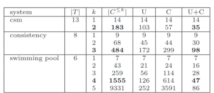
system |T | k |C≤k| U C U+C csm 13 1 14 14 14 14 2 183 103 57 35 consistency 8 1 9 9 9 9 2 68 45 44 30 3 484 172 299 98 swimming pool 6 1 7 7 7 7 2 43 21 24 16 3 259 56 114 28 4 1555 126 614 47 5 9331 252 3591 86
|C≤k| : number of valid circuits of length ≤ k
U: number of valid circuits after the reduction by union C: number of valid circuits after the reduction by commutation U+C: number of valid circuits after the reduction by union and commutation
Table 3.Effect of circuit reductions on case-studies
guards f1 = (ϕ1, M, −→v) and f2 = (ϕ2, M, −→v) into a
unique affine function f1+ f2= (ϕ1∨ ϕ2, M, −→v).
Reduction by commutation consists in removing tran-sitions g · f and f · g, where f, g ∈ T≤k for some k,
whenever f and g satisfy −−→=f·g −−→. This is soundg·f w.r.t. reachability since (−−→)f·g ∗ and (−−→)g·f ∗ are then
equal to (−→)f ∗• (−→)g ∗.
In [37], it is proven that reduction by union reduces the number of cycles of length ≤ k of linear counter systems with finite monoid to a polynomial number in k. Table 3 shows the effect of these reductions on a few examples. The bold value of k indicates the length of circuits used by Fast to compute the fixpoint.
Both reduction techniques appear to perform well in practice, and their combination leads to impressive cut-offs: |C≤k| is divided by 5 in the first two examples,
and by 30 in the last one. Reductions are definitely a key feature in Fast performances, allowing the tool to consider circuits of length 4 or 5 in some examples. Beyond flat acceleration. The reduction by union al-lows to compute some particular kinds of nested loops. Actually, when considering linear counter systems with guards defined over the full binary automata logic, the union reduction allows to compute the reachability set of non-flattable counter systems. The question is still open for standard linear counter systems.
5.5 Flattable systems almost everywhere!
The question “Given a linear counter system with fi-nite monoid S, is S flattable?” is undecidable, since the reachability problem reduces to this question [7]. How-ever many interesting subclasses of counter systems have been shown to be flattable. It is the case for 2-dim VASS [56], k-reversal counter machines, lossy VASS, Cyclic VASS and other subclasses [57].
This is interesting for at least two reasons. From a practical point of view, procedure 2 provides a unified
and efficient algorithm to decide reachability on all these subclasses of counter systems. This is an important step, since even though most of these subclasses were known to be decidable, their algorithms were totally different and very difficult to extend. From a theoretical point of view, it is interesting to note that some of the previous proofs of reachability used specific cases of circuit accel-eration and flattening. These proofs are easier to write once these concepts are clearly identified.
6 FAST: Tool description
Fast[5,9] is a tool for checking safety properties of linear counter systems. The tool is designed according to the flat acceleration framework.
6.1 Computational framework
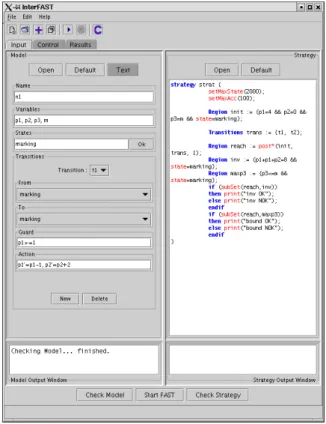
Fast is organized through a client-server architecture. The server is the computation engine as described in section 6.1. It contains a Presburger library, the accel-eration algorithm and the search heuristics. The client is a front-end which allows the user to interact with the server through a graphical user interface (GUI, figure 5). The server can also be used as a standalone tool. The server is written in C++ (7, 400 lines) while the client is written in Java. The Mona library [53,61] provides basis for automata manipulations.
6.1.1 Software architecture
Fastengine is structured according to the flat acceler-ation framework. The program is organized around four main classes: Presburger-affine functions, ndd, accelera-tion algorithms and a flattening heuristic.
ndd are encoded in basis 2, least-digit first. The class provides standard set operations like union, intersection, complementation and projection, as well as the synthesis of a ndd from a Presburger formula. This implementation is built on the Mona package. Note that for efficiency purposes, Mona restricts automata to 224nodes.
Standard acceleration and convex acceleration algo-rithms are implemented, which can be used for both forward and backward computation.
The flattening heuristic follows procedure 2. Reduction by commutation and reduction by union are both avail-able.
6.1.2 Technical issues
Procedure reach2, data structures and algorithms pre-sented in sections 3 and 4 provide the backbone of Fast. However, several practical problems are not covered by
these results. For example, locations can be encoded ex-plicitly or by counters, circuits can be computed stati-cally or on-the-fly. Here, we describe some implementa-tion choices made in Fast. Currently there is no known best solution for each of the problems mentioned here-after.
Variables in N. All the results of sections 3 and 4 hold for variables ranging over Z. However in Fast counters range over N. First, the corresponding ndd are smaller thanks to a simpler encoding, which leads to better per-formance. Second, this is not a strict restriction since we did not find any example where negative counters were required and moreover a variable x ∈ Z can always be encoded by two positive variables x+, x−∈ N such that
x= x+− x− and (x+= 0 ∨ x− = 0).
Location encoding. A stated in remark 1 (page 4), boun-ded variables (control, boolean, bounboun-ded integer vari-ables) are encoded as counter variables. On the one hand it allows for a better sharing of the reachability set struc-ture and avoids an explicit product of control strucstruc-tures for systems composed of many components. On the other hand, we do not take any advantage of the boundedness of these variables. A solution may be to extend ndd with a bdd-like structure for bounded variables, following the work done in [11].
Static computation of circuits. We compute statically circuits of length k. Practical case studies show that this approach is tractable thanks to reductions. However dis-covering circuits on-the-fly, or at least a dynamic slicing of potential circuits, would probably be useful.
6.2 Input/Output
Fasttakes as input a description of the system to be an-alyzed and a strategy specifying what to compute. Out-puts are textual messages stating if the system is safe or not. Finally, a graphical user interface is also available. 6.2.1 The input system
The linear counter system can be described directly in the Fast formalism. However since many of Fast’s case studies were extended Petri nets, we developed a tool [10] to transform a Petri net in pnml format into a Fast model. The language pnml [16] describes various exten-sions of Petri nets and is being standardized (ISO/IEC 15909-2).
6.2.2 The strategy
The strategy is a script specifying the sequence of com-putations to perform in order to prove the correctness of the system. This script language manipulates sets of con-figurations (region), sets of transitions (transition)
and booleans. All basic set-operations are available. The user can define finite sets of transitions T′ ⊆ T∗ and
primitives to compute post∗(T′, X0) and pre∗(T′, X0) are
provided. A standard forward analysis is specified us-ing only four instructions: declare the initial region X0,
compute the reachability set post∗(T′, X
0), declare the
region P describing the property to check and finally test whether post∗(T′, X
0) ⊆ P .
The language also allows the user to guide the tool more precisely. For example a system can be analyzed in an incremental way, dividing the whole system into smaller parts (cf. section 9); the user can indicate circuits to be used; choose the acceleration algorithm; or set up parameters of the heuristics.
The script language gives the user control over the se-quence of computations performed. This can prove use-ful when the use-fully automatic approach fails. Thus, Fast stands between a fully automatic approach, justified when termination is guaranteed but restrictive otherwise, and computer-aided verification.
6.2.3 User Interface
A graphical user interface [6] is available (see figure 5). It provides aided editing of systems and strategies, pretty printing, and predefined strategies. Once the computa-tion starts, the interface supplies the user with feedback on a number of parameters (memory consumption, time elapsed, etc.).
6.3 FAST Extended Release
An extended version of Fast has been presented in [9]. This new release offers mainly an open architecture al-lowing to plug easily any Presburger package to the tool. Open architecture. The architecture has been slightly redesigned and is now divided into two parts: on the one side, a counter system analysis engine built upon a generic Presburger API (instead of a ndd package); on the other side, various implementations of this API. The generic Presburger programming interface (Genepi) re-quires only basic set-theoretic operations on Presburger-definable sets. We provide three implementations of the API based on standard packages Lash [55], Mona [61] and Omega [62]. The first two packages are automata-based while Omega is formula-automata-based. The Mona imple-mentation corresponds to the original version of Fast. All experiments carried out in this paper use the Mona implementation.
The shared automata package. An implementation of the API using shared automata introduced by Couvreur in [28] has been developped by J´erˆome Leroux and G´erald Point. These automata share their strongly connected
Fig. 5: Fast graphical user interface
components in a bdd-like manner, allowing to implement important features for intensive computation, such as cache computation and constant-time equality testing. The library is functional, but the computation cache is not sufficiently optimized yet. The shared automata package is called PresTaf.
Experimental comparisons performed in [9] demonstrate that the three automata-based implementations of the generic Presburger API largely outperform the formula-based implementation. Indeed Omega appears to com-pute unduly complicated Presburger formulas (even with the simplification method provided by the package), while Lash, Mona and PresTaf benefit from canonical rep-resentations of automata.
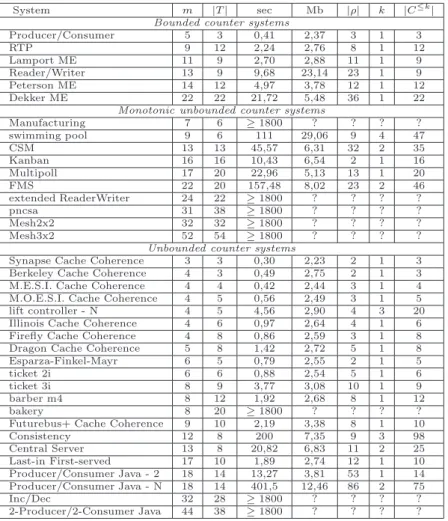
7 Experiments
This section reports some experiments made with Fast. 7.1 About tests
We use a large pool of counter systems and case studies
analyzed by tools Alv, Babylon3, Brain, Lash and
TReXto evaluate Fast. These 37 systems are available on Fast web pages [35].
3
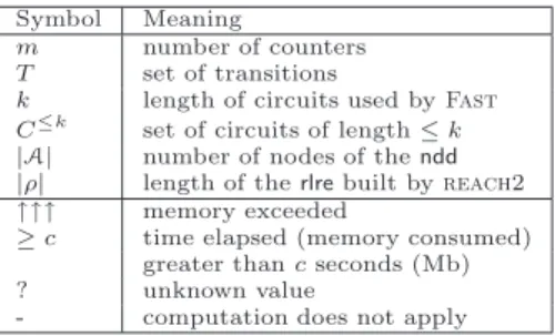
Symbol Meaning
m number of counters T set of transitions
k length of circuits used by Fast C≤k set of circuits of length ≤ k
|A| number of nodes of the ndd |ρ| length of the rlre built by reach2 ↑↑↑ memory exceeded
≥ c time elapsed (memory consumed) greater than c seconds (Mb) ? unknown value
- computation does not apply
Table 4.Symbols used in test reports
These systems range from tricky academic puzzles like the swimming pool protocol [42] to industrial case stud-ies like the cache coherence protocol for the Futurebus+. We distinguish three categories of systems: counter sys-tems with a finite reachability set, monotonic counter systems with an infinite reachability set and linear counter systems with an infinite reachability set.
All experiments have been performed on an Intel Pen-tium III 933Mhz equipped with 512 Mbytes of memory. Time is in seconds and memory in Mbytes. Fast is used with the following settings: standard acceleration, basic strategy (no human guidance), Mona-based implemen-tation of the Presburger API.
7.2 Results
Table 5 reports Fast behavior on the examples, us-ing forward computation. The number of cycles |C≤k| is
given after reductions (union and commutation). Fastcomputes successfully the reachability set of 78% of the systems considered. This ratio is 74% when con-sidering only unbounded systems. We show in section 8 that Fast performs better than similar tools.
These good results validate the design of Fast. First, all examples are expressed straightforwardly by means of counter systems. Second, the monoid is always finite. At least 78% of the systems are flattable and have a Presburger-definable reachability set. Finally in 19% of the tests, the length of circuits used is strictly greater than 1. This number increases to 22% when considering only unbounded counter systems. This proves that con-sidering circuits and not only loops is a major feature.
Fastlimitations are likely to be more practical (mem-ory consumption, time elapsed) than theoretical. Crucial points are not only the number of variables, but also (and mainly!) the structure of the reachability set and the length k of the circuits used. Indeed, when k is too large, the static computation of circuits consumes too many resources.
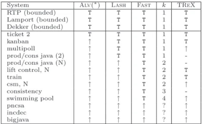
8 Comparison with other tools
In this section, we compare Fast with other tools, namely Alv, Lash and TReX, to evaluate their performance on exact forward reachability set computation. Let us pin-point that the goal here is not to find out which tool is the best for counter system validation. Actually, it would be unfair for TReX which is mostly designed for timed automata extended with integer variables, and for Alv which offers full CTL model checking, backward compu-tation, over-approximation and different symbolic repre-sentations. These experiments are rather used to evalu-ate the contribution of each particular feature of Fast. 8.1 The tools
First, we present the tools Alv, Lash and TReX, and compare them with Fast through the flat acceleration framework.
Alv [25,68] is designed to check any CTL formula on full counter systems. Alv also offers different sym-bolic representations for integer vectors (automata or Presburger formula) and a wide range of options, like backward computation, over-approximation [12] for the automata-based representation and accelera-tion [50] for the formula-based representaaccelera-tion. This acceleration algorithm is designed for the following class of operations: there is no guard and actions are mostly relations of the form x′
i#xi + c where
# ∈ {≤, =, ≥} and x′
iis the value of variable xiafter
the transition occurs. Typically Alv uses approxi-mate forward fixpoint computation to prune the state space during the backward fixpoint computations. In the rest of the paper, we use the following config-uration: automata-based representation (then no ac-celeration), forward computation, no over-approximation. In this configuration, the main differences with Fast are that no acceleration algorithm is available, the heuristic is similar to reach1 and bounded variables are encoded by bdd [11].
Lash [55] works on linear counter systems. Regions are encoded by automata and standard acceleration is implemented for functions with a finite monoid. Without user guidance, Lash is restricted to loop acceleration (i.e. the heuristic considers only words w∈ T instead of sequences in T∗) because no circuit
search is supplied.
TReX [3] manipulates counter systems restricted to timed automata-like operations4: guards are
conjunc-tions of constraints xi− xj≤ c and actions are of the
form x′
i= xj+c where xiis a variable, c is a constant
and xj is a variable or the constant 0. Regions are
en-coded by pdbm, an extension of dbm with additional 4
Actually TReX is designed to check systems with clocks and counters. We consider here the restriction to counter systems.
System m |T | sec Mb |ρ| k |C≤k| Bounded counter systems
Producer/Consumer 5 3 0,41 2,37 3 1 3 RTP 9 12 2,24 2,76 8 1 12 Lamport ME 11 9 2,70 2,88 11 1 9 Reader/Writer 13 9 9,68 23,14 23 1 9 Peterson ME 14 12 4,97 3,78 12 1 12 Dekker ME 22 22 21,72 5,48 36 1 22
Monotonic unbounded counter systems
Manufacturing 7 6 ≥ 1800 ? ? ? ? swimming pool 9 6 111 29,06 9 4 47 CSM 13 13 45,57 6,31 32 2 35 Kanban 16 16 10,43 6,54 2 1 16 Multipoll 17 20 22,96 5,13 13 1 20 FMS 22 20 157,48 8,02 23 2 46 extended ReaderWriter 24 22 ≥ 1800 ? ? ? ? pncsa 31 38 ≥ 1800 ? ? ? ? Mesh2x2 32 32 ≥ 1800 ? ? ? ? Mesh3x2 52 54 ≥ 1800 ? ? ? ?
Unbounded counter systems
Synapse Cache Coherence 3 3 0,30 2,23 2 1 3
Berkeley Cache Coherence 4 3 0,49 2,75 2 1 3
M.E.S.I. Cache Coherence 4 4 0,42 2,44 3 1 4
M.O.E.S.I. Cache Coherence 4 5 0,56 2,49 3 1 5
lift controller - N 4 5 4,56 2,90 4 3 20
Illinois Cache Coherence 4 6 0,97 2,64 4 1 6
Firefly Cache Coherence 4 8 0,86 2,59 3 1 8
Dragon Cache Coherence 5 8 1,42 2,72 5 1 8
Esparza-Finkel-Mayr 6 5 0,79 2,55 2 1 5
ticket 2i 6 6 0,88 2,54 5 1 6
ticket 3i 8 9 3,77 3,08 10 1 9
barber m4 8 12 1,92 2,68 8 1 12
bakery 8 20 ≥ 1800 ? ? ? ?
Futurebus+ Cache Coherence 9 10 2,19 3,38 8 1 10
Consistency 12 8 200 7,35 9 3 98 Central Server 13 8 20,82 6,83 11 2 25 Last-in First-served 17 10 1,89 2,74 12 1 10 Producer/Consumer Java - 2 18 14 13,27 3,81 53 1 14 Producer/Consumer Java - N 18 14 401,5 12,46 86 2 75 Inc/Dec 32 28 ≥ 1800 ? ? ? ? 2-Producer/2-Consumer Java 44 38 ≥ 1800 ? ? ? ?
Table 5.Fastin practice
parameters constrained by an arithmetic formula. An acceleration procedure is implemented, which allows at least all accelerations of Fast and Lash. However this procedure produces unrestricted arithmetic for-mulas and then inclusion becomes undecidable. The heuristic is restricted to C≤k, for a value of k
stat-ically defined by the user. Finally, TReX does not compute circuits statically but discovers them on-the-fly. A more in-depth comparison of Fast and TReXis presented in [29].
Table 6 compares the different tools through the flat acceleration framework. Column “termination” indicates the class of systems for which the tool terminates (F: flattable, k-F: k-flattable, Unif-b: uniformly bounded).
8.2 Comparison on forward computation
We now compare the capabilities of Alv, Lash, Fast and TReX in exact forward computation of reachability sets. The counter systems chosen for tests all have an infinite reachability set, except systems RTP, Lamport and Dekker. Results are summarized in table 7.
sy st e m sy m b . re p . a c c e le ra ti o n te rm in a ti o n
Alv full ndd no Unif-b
Fast linear ndd flat F
Lash linear ndd loop 1-F
TReX restricted pdbm interpolation k-F (∗)
(∗) Termination modulo an oracle to decide inclusion.
Table 6.Different tools for the verification of counter systems.
Experimental results show a drop in performance of Alvand Lash when k increases. Fast completely sup-ports the flat acceleration framework and obtains the best results. On the other side, Alv does not supply any acceleration mechanism and the tool does not succeed in computing these complex reachability sets. Between Alv and Fast, the tool Lash is restricted to loop accelera-tion and it terminates only on simple examples (k ≤ 1). Note that when Lash is provided with the circuits to use, its performance is similar to that of Fast. The dif-ference between Fast and Lash is primarily the length of circuits, not the ndd implementation. Finally, TReX performance is less correlated with k, since the tool
ter-System Alv(∗) Lash Fast k TReX RTP (bounded) T T T 1 T Lamport (bounded) T T T 1 T Dekker (bounded) T T T 1 T ticket 2 T T T 1 T kanban ↑ T T 1 T multipoll ↑ T T 1 ↑ prod/cons java (2) ↑ T T 1 -prod/cons java (N) ↑ ↑ T 2 -lift control, N ↑ ↑ T 2 T train ↑ ↑ T 2 T csm, N ↑ ↑ T 2 ↑ consistency ↑ ↑ T 3 -swimming pool ↑ ↑ T 4 ↑ pncsa ↑ ↑ ↑ ? ↑ incdec ↑ ↑ ↑ ? ↑ bigjava ↑ ↑ ↑ ? ↑
T: computation of the reachability set in less than 20 minutes ↑: no termination in less than 20 minutes
- : the systems cannot be modeled in TReX
(∗) These results are consistent with those reported by Bultan and
Bartzis in [12].
Table 7.Comparison of different tools
minates for the lift system (k = 2) and fails on multipoll (k = 1).
These results demonstrate a strong correlation between the flat acceleration framework and practical termina-tion. Comparison between Alv and Lash shows the ben-efits of acceleration, while comparison between Lash and Fasthighlights the necessity of selecting circuits and not only loops.
TReXresults show that pdbm is not a good symbolic framework for counter systems, since many systems can-not be modeled this way and moreover, despite acceler-ation, termination occurs less frequently. Again, recall that TReX is primarily designed to handle parametric timed systems.
8.3 Comments
Fastappears to be a very efficient tool for the forward computation of reachability sets of counter systems. In experiments, Fast performance is clearly superior to that of similar tools Alv, Lash and TReX.
Again, recall that it does not necessarily imply that Fastis better then the other tools for counter systems validation since we restricted the experiments to exact forward computation while other approaches exist. More-over, recall that we use restrictions of Alv and TReX which are primarily designed to handle different systems (TReX) or richer properties (Alv). Yet, we believe that the computation of the exact reachability set of a linear counter system is an important issue and in this setting, technologies implemented in Fast are clearly superior.
9 The TTP protocol
This section describes the verification of the TTP pro-tocol with the tool Fast. In prior work the propro-tocol was verified correct by hand (for an arbitrary number of faults) or in a computer-aided manner (for one fault) with Lash and Alv. These tools could not verify cor-rectness for two faults. Fast checks automatically the correctness of the protocol for one fault, and correctness is proved for two faults, using abstractions.
9.1 Protocol description
The TTP protocol [54] is supported by the transport industry (Airbus, Audi, EADS, PSA and others) and aims at managing embedded microprocessors. We focus here on the group membership algorithm of the TTP. It is a fault-tolerant algorithm, preventing the partitioning of valid microprocessors (stations) after a failure.
A clique is a subset of stations communicating only with stations of the same clique. In normal behavior, there is only one clique containing all the valid stations. The protocol ensures that when a fault occurs and cre-ates different cliques among the stations, after a while valid stations belong to a unique clique.
Description. Time5 is divided into rounds. Each round
is divided into as many slots as stations. The protocol behaves as follows (a more complete description can be found in [54,22]):
1. Each station si keeps the following information: a
list li of boolean values stating, for each station sj,
whether si considers sj as valid or not; two counters
CAcki and Ci F ail.
2. During a slot, only one station broadcasts a message and the others receive it. The message is the list li.
3. When a station sj receives a message from a station
si: if li 6= lj, or if no message is received, then sj
considers si as faulty; lj is updated and CF ailj is
in-cremented. Otherwise CAckj is incremented.
4. When a station si is about to broadcast a message:
if Ci
Ack≤ CF aili then siconsiders itself as invalid and
becomes inactive (no emission). Otherwise Ci Ackand
Ci
F ailare reset to 0, and liis broadcasted to all other
stations. 9.2 Modeling
We use the modeling proposed by Merceron and Boua-jjani in [22]. This modeling is based on counter systems. It captures an arbitrary number N of stations but only
5
Clocks are synchronized by other mechanisms of the TTP pro-tocol.
a fixed number of faults. Merceron and Bouajjani actu-ally provide an infinite family of counter systems, each modeling the behavior of the protocol for some number f of faults.
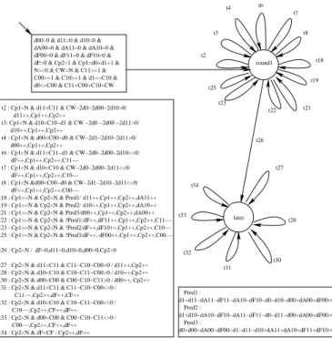
The counter system for f = 1 is given in figure 6. Vari-able Cw(resp. CF) denotes the number of active stations
(resp. inactive stations). Variable Cp counts the number
of slots elapsed during the round. Since a round is di-vided into N slots, when Cp = N , variable Cp is reset
to 0 and a new round begins. Location normal models the normal behavior of the protocol. When a fault oc-curs, the protocol enters abnormal behavior. Location Round1 is the first round following the error. Location later represents the other rounds. A fault divides ar-bitrarily active stations into two cliques C1and C0. We
denote by C1 and C0 the number of stations of cliques
C1and C0. Variable d (resp. d0, d1, dF) counts the
num-ber of active stations (resp. from C0, from C1, inactive)
which have emitted during the round.
/ CF=0,CW=N,Cp=0 d=0,dF=0 / C1>=0, C0>=0, C1+C0=CW, d1=1,d0=0, dF=0,Cp=1 later round1 normal init d=0,dF=0 Cp=N / CW=C1+C0,Cp=0, Cp=0,d=0,dF=0 Cp=N / dF<CF / dF++, Cp++ d1<C1 & C1+C0−2d0>0 / d1++, Cp++ C1−−,dF++,CF++,Cp++ d1<C1 & C1+C0−2d0<=0/ d0<C0 & C1+C0−2d1>0 / d0++, Cp++ d0<C0 & C1+C0−2d1<=0 / C0−−,dF++,CF++,Cp++ dF<CF / dF++,Cp++ d1++,Cp++ d1<C1 & C1>C0 / d1<C1 & C1<=C0 / C1−−,CF++,dF++,Cp++ d0<C0 & C0>C1 / d0++,Cp++ d0<C0 & C0<=C1 / C0−−, CF++, dF++,Cp++ Cp=N & !(C1=0) & !(C0=0) / d1=0,d0=0,dF=0,Cp=0 d<CW / d++,Cp++ dF<CF / dF++,Cp++ Cp=N / d1=0,d0=0,dF=0,Cp=0
Fig. 6: Model for the TTP, 1 fault
The safety property to check is that, at most two rounds after the fault occurs, there is only one clique left. It is expressed in this model by the following property (P1) : location = later ∧ Cp = N ⇒ (C1= 0 ∨ C0= 0).
Remark 6. This specification is actually incomplete, and we should check: For all paths, if a fault occurs then lo-cation later is reached and property P1 holds. However
this property is not a safety property. Model checking tools for infinite state systems such as Alv can han-dle these type of properties which cannot be hanhan-dled by reachability tools such as Fast.
Interests of this case study. The number of counters is not large (9), and actions are standard. However guards are complex linear inequalities involving many variables.
The counter system is not an extended VASS nor a re-stricted counter system manipulated by TReX. More-over, because of the strong connection between variables, the reachability set has a very complex structure. How-ever, it is Presburger-definable.
9.3 Automatic verification for 1 fault
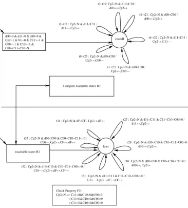
The counter system of figure 6 is not linear because of the non-deterministic assignment of the transition be-tween location normal and location Round1. Hopefully, since the transition between later and normal models returning back to the normal mode, property P1 is only
concerned with what happens in later, and variables af-fected non deterministically are not used in normal, we can remove this transition. Then the non deterministic assignment can be encoded into the initial region.
The resulting linear counter system is presented in fig-ure 7. This system has a finite monoid.
later round1 normal init Cp=0,d=0,dF=0 Cp=N / dF<CF / dF++, Cp++ d1<C1 & C1+C0−2d0>0 / d1++, Cp++ C1−−,dF++,CF++,Cp++ d1<C1 & C1+C0−2d0<=0/ d0<C0 & C1+C0−2d1>0 / d0++, Cp++ d0<C0 & C1+C0−2d1<=0 / C0−−,dF++,CF++,Cp++ dF<CF / dF++,Cp++ d1++,Cp++ d1<C1 & C1>C0 / d1<C1 & C1<=C0 / C1−−,CF++,dF++,Cp++ d0<C0 & C0>C1 / d0++,Cp++ d0<C0 & C0<=C1 / C0−−, CF++, dF++,Cp++ Cp=N & !(C1=0) & !(C0=0) / d1=0,d0=0,dF=0,Cp=0 / C1>=0, C0>=0, C1+C0=CW, d1=1,d0=0, dF=0,Cp=1 CF=0,CW=N,Cp=0 d=0,dF=0 d<CW / d++,Cp++ Cp=N / d1=0,d0=0,dF=0,Cp=0 dF<CF / dF++,Cp++
Fig. 7: Linear counter system for the TTP, 1 fault
Results. Fast checks automatically that property P1is
satisfied. The computation of the reachability set re-quires only cycles of length 1, and the minimal ndd com-puted has 27, 932 nodes. Computation takes 1, 880 sec-onds and 73 Mb of memory.
Incremental analysis. The computation time can be re-duced via a better script strategy. Indeed, Fast heuristic does not take into account the particular aspect of the control graph of the protocol. Since there is no return-ing back in the graph, we can first compute the set of all configurations reachable on location normal, then fire the transition to reach location Round1, and iterate the process. This decomposition is made explicit in figure 8.