Cooling system early-stage design tool for naval applications

Cooling System Early-Stage Design Tool

For Naval Applications

By

Ethan R. Fiedel

Bachelor of Science in Naval Architecture

United States Naval Academy, 2001

MASSAHUSETTS INSTITUTE OF TECHNOLCGY

J1JL 2~

2011

L BRA RIE S

ARCHNVES

Submitted to the Department of Mechanical Engineering

In Partial Fulfillment of the Requirements for the Degrees of

Naval Engineer

and

Master of Science in Mechanical Engineering

at the

Massachusetts Institute of Technology

June 2011

C 2011 Ethan Fiedel. All rights reserved.

The author hereby grants to MIT permission to reproduce and to distribute publicly paper and electronic copies of this thesis document in whole or in part in any medium now known or hereafter created.

Signature of Author

Ethan R. Fiedel Department of Mechanical Engineering May 6, 2011

-

t

Certified by

Chryssostomos Chryssostomidis Thesis Supervisor Professor of Mechanical and Ocean Engineering

Accepted by 1% V dt

-01 1, P17David Hardt

Chairman, Committee for Graduate Students Department of Mechanical Engineering %.. W --VI _

(THIS PAGE INTENTIONALLY LEFT BLANK)

Cooling System Early-Stage Design Tool

For Naval Applications

Ethan R. Fiedel

Submitted to the Department of Mechanical Engineering in Partial Fulfillment of the Requirements for the Degrees of

Naval Engineer

and

Master of Science in Mechanical Engineering

Abstract

This thesis utilizes concepts taken from the NAVSEA Design Practices and Criteria Manualfor Surface

Ship Freshwater Systems and other references to create a Cooling System Design Tool (CSDT). With the

development of new radars and combat system equipment on warships comes the increased demand for the means to remove the heat generated by these power-hungry systems. Whereas in the past, the relatively compact Chilled Water system could be tucked away where space was available, the higher demand for chilled water has resulted in a potentially exponential growth in size and weight of the components which make up this system; as a result, the design of the cooling systems must be considered earlier in the design process. The CSDT was developed to enable naval architects and engineers to better illustrate, early in the design process, the requirements and characteristics for the Chilled Water system components. Utilizing both Excel and Paramarine software, the CSDT rapidly creates a visual model of a Chilled Water system and conducts pump, damage, cost, weight, and volume analyses to assist in further development and design of the system.

Several case studies were run to show the capability and flexibility of the tool, as well as how new electronic and mechnical systems can affect the parameters of the Chilled Water system.

Thesis Supervisor: Chryssostomos Chryssostomidis Title: Professor of Mechanical and Ocean Engineering

(THIS PAGE INTENTIONALLY LEFT BLANK)

Table of Contents

Executive Sum m ary...13

1.0 Introduction ... 15

1.1 Organization of Thesis... 15

1.2 Topic M otivation...15

1.3 Background ... 16

1.4 Thesis Intent ... 22

2.0 Design Tool Concepts... 23

2.1 Pipe and Valve Characteristics ... 23

2.2 Air Conditioning Plant Sizing ... 27

2.3 Pum p Powering Com parison... 29

2.4 Expansion Tank Design... 37

2.5 Dam age Analysis ... 40

2.6 Cost Analysis ... 44

3.0 Design Tool Explanation... 46

3.1 Program Requirem ents and Lim itations ... 46

3.2 Program Operations... 49

4.0 Case Studies and Tradeoffs... 55

4.1 Com parison of the CSDT Results Against Existing Ship Data ... 55

4.2 Zone Com parison Analysis ... 58

4.3 AC Plant Type Com parison ... 60

4.4 AC Plant Size Com parison ... 61

5.0 Conclusions ... 63

5.1 General Conclusions... 63

5.2 Areas of Future Study... 63

R e fe re n ce s ... 6 5 Appendix A: Program Instruction M anual ... 67

Appendix B: CSDT Entry, Analysis, and Output W orksheets... 76

B-1: "Procedure" W orksheet ... 77 B-2: "ZonalData" W orksheet... 83 B-3: "LoadData" W orksheet... 85 B-4: "Sheetla" W orksheet ... 91 B-5: "AC H X" W orksheet ... 95 B-6: "Sheetib" W orksheet... 98

B-7: "Dam age" W orksheet... 101

B-8: "Sheet1" W orksheet ... 104

B-9: "Pum p" W orksheet... 106

B-10: "Cost Analysis" W orksheet ... 109

Appendix C: CSDT Code... 110

List of Figures

Figure 1: Typical marine AC plant refrigerant cycle. (Taylor, 1990)... 17

Figure 2: Design Spiral. (Society of Naval Architects and Marine Engineers, 2003)...19

Figure 3: a) and b) ASSET plan and profile view of destroyer; c) and d) ASSET plan and profile view of M M R 2 ... 2 1 Figure 4: Non-dimensionalized plots detailing how the AC plant parametrics, for the two types of plants, w e re d ete rm ined . ... 28

Figure 5: Sam ple pum p characteristic curve (Franzini, 1997)... 29

Figure 6: Moody chart for pipe friction factor (Franzini, 1997)... 32

Figure 7: Plots obtained from pulling points from the Moody Diagram at a) 12 fps and b) 9 fps...32

Figure 8: Entrance loss coefficients (Franzini, 1997) ... 34

Figure 9, a) Pump head and capacity as a function of speed: Top = 1750 RPM, Middle = 1150 RPM, Bottom = 3500 RPM; b) Expanded 1750 RPM plot with the provided conditions highlighted in red; c) expanded plot of the pump which meets the needs of the system. (ITT Industries: Bell & Gossett, 1998) ... 3 5 Figure 10, Pump curves for the 1510 Series 5E pump at 1750 RPM. The red lines indicate the requirements for the designed condition (ITT Industries: Bell & Gossett, 1998)... 35

Figure 11, Pum p efficiency chart ... 37

Figure 12, An example of the increased durability cabinets and the rigorous testing they undergo. (G lobal Technical System s (GTS), 2010)... 41

Figure 13: Damage analysis data entry section of the CSDT... 42

Figure 14: CSDT dam age analysis output... 42

Figure 15, Excel output for input to MATLAB damage analysis code ... 44

Figure 16: a) Cross connect piping within a zone; b) Cross connect piping across zones ... 48

Figure 17: Piping/Electrical service highway for a notional frigate ... 49

Figure 18: a) Data entry cell unselected; b) data entry cell selected; c) data entry cell with menu button se le cte d ... 5 2 Figure 19: a) Default value settings (top); b) manual data entry values (bottom)... 52

Figure 20: Sample Paramarine piping visualization generated by the CSDT. ... 53

Figure 21: Sample Paramarine system characteristic table generated by the CSDT... 53

Figure 22: Illustration of the initial placement of the chilled water piping (green) external to the hull.... 54

Figure 23, Visual output from Param arine ... 57

Figure 24, Paramarine visual outputs for the a) Type "A" AC plant and b) Type "B" AC plant ... 61

Figure 25: Minimum Paramarine setup requirements. The image on the right shows the major folders exp a n d e d. ... 67

Figure 26: Paramarine setup as created in the aforementioned tutorial ... 68

Figure 27: Illustration of Step 2... 68

Figure 28: Step 5 W arning box... 69

Figure 29: a) (Left) Cooling Loop with Ends at the bow and stern, b) (Right) Cooling Loop with branches running to the bow and stern ... 69

Figure 30: Cooling system loading for each of the four operational conditions. Also shown is the data entry highlighted cell referenced in sub-step "b"... 71

Figure 31: a) (Left) Resulting image in data entry area of AC-HX tab if 11.b is set to 3 and 11.d is set to 2; b) (Right) Resulting image of data entry are of AC-HX tab if 11.b is set to 2 and 11.d is set to 1...72

Figure 32, Step 7 output sam ple ... 73

Figure 33: Example of the folder setup and piping layout generated within/by Paramarine...74

Figure 34: Example of the folder setup and weight output generated within/by Paramarine...74

Figure 35: File folder to control positions and locations of the chilled water zones and headers...75

Figure 36, Procedure W orksheet layout ... 77

Figure 37, LoadData W orksheet layout ... 85

Figure 38: Sheetla W orksheet layout... 91

Figure 39: AC_ HX W orksheet layout... 95

Figure 40: Sheet1b W orksheet layout ... 98

Figure 41: Dam age W orksheet layout ... 101

List of Tables

Table 1: Dimensions and weights of copper-alloy number 715 (MIL-T-16420K-1, 1978) ... 24

Table 2: Span between supports. (Anvil International, 2007) ... 25

Table 3, Dimensions and weight characteristics for RAKO Valves' WJ41-150LB model valve (RAKO Valve) ... _{2 6} Table 4: Various configurations of AC plant capacities and numbers of plants ... 27

Table 5: Values of loss factors for pipe fittings (Franzini, 1997)... 33

Table 6, Weights for the Series 1510 5E pump (ITT Industries: Bell & Gossett, 1998)... 36

Table 7: Volume and expansion of water in piping (32*F to 120*F) (NAVSEA, 1987)... 39

Table 8, Chilled water plant costs estimated (Trane, 2000)... 44

Table 9: Sum m ary of CSDT input and output tabs... 51

Table 10, Entering factors for the first case study ... 56

Table 11, Weight comparison between CSDT and SWBS data ... 56

Table 12, Volume comparison between ASSET derived system volume and CSDT system volume ... 57

Table 13, Input data for zonal case study ... 58

Table 14, Zone case study results ... 59

Table 15, AC plant com parison case study ... 60

Table 16, Plant size com parison case study results ... 62

Acronym List

ASSET Advanced Surface Ship Evaluation Tool

ASW Auxiliary Sea Water

CFC Chlorofluorocarbons

CSDT Cooling System Design Tool

ESRDC Electric Ship Research and Design Consortium

HFC Hydrofluorocarbon

LBP Length Between Perpendiculars

LOA Length Overall

LT Long Tons

MIT Massachusetts Institute of Technology

MSW Main Sea Water

NAVSEA Naval Sea Systems Command

NARC Naval Architect

NPSH Net Positive Suction Head

OS Operating System

P&A Payload and Adjustments

POSSE Program Of Ship Salvage Engineering

SWBS Ships Work Breakdown Structure

Te Metric Tons

Biographical Note

Ethan Fiedel is an active duty Navy Lieutenant currently pursuing a degree in Naval Engineering,

Mechanical Engineering, and Engineering and Management as prerequisites for subsequent assignment as an Engineering Duty Officer. His past assignments include sea and shore assignments attached to USS

PROVIDENCE (SSN-719), Commander Submarine Squadron (COMSUBRON) 22, and Commander Task

Force (CTF) 69.

Lieutenant Fiedel's most recent assignments include Submarine Watch Officer for SIXTH FLEET. Previously, he was assigned as the Operations Officer for COMSUBRON 22. Other assignments include Communications Officer, Damage Control/Auxiliary Division Officer, Main Propulsion Assistant, and Electrical Officer onboard a nuclear powered submarine.

Lieutenant Fiedel is a graduate of the Prospective Nuclear Engineer Officer Course, Submarine Officer Basic Course, and the Naval Nuclear Propulsion Course. His awards and decorations include the Navy Commendation Medal, four Navy Achievement Medals, and the Submarine Warfare Qualification.

Lieutenant Fiedel graduated from the United States Naval Academy in 2001 with a Bachelor of Science Degree with Merit in Naval Architecture. This work completes the requirements for his Naval Engineers Degree and Masters of Science in Mechanical Engineering at the Massachusetts Institute of Technology.

Acknowledgements

I would like to first thank my wife, Jennifer, who has endured the highs and lows of life by my

side and brought me joy when I needed it the most; no person could continue to give more (as this is the second thesis) and ask for less as she put her career second, withstood the late night returns and early

morning departures.

I also would like to thank my parents, Robert and Susan, who have supported me throughout

this and all of my endeavors.

This project would not have been remotely possible without the support, kindness, and donation of time by several of the staff members of NAVSEA engineering branches and Alion Science and Technology.

Finally, I could not have completed this project without the support and guidance of my advisors, Professor Chryssostomos Chryssostomidis and Julie Chalfant. Their guidance and patience enabled me to complete this work, without beating my head against the wall too hard.

(THIS PAGE INTENTIONALLY LEFT BLANK)

Cooling System Early-Stage Design Tool

For Naval Applications

Ethan R. Fiedel

Submitted to the Department of Mechanical Engineering

In Partial Fulfillment of the Requirements for the Degrees of

Naval Engineer

and

Master of Science in Mechanical Engineering

Executive Summary

Available to the general public are guidebooks and references for designing cooling water systems for naval warships; key among these resources is the Naval Sea Systems Command (NAVSEA)

Design Practices and Criteria Manualfor Surface Ship Freshwater Systems. While this manual lists the

steps required and provides selected equations and thumbrules for selecting components in cooling water systems, it does not design an overall system nor does it define the overall characteristics of a system (i.e. weight, volume, cost, etc.); with the development of new, higher heat generating radars and combat system equipment, there is an increased demand for chilled water, which implies a larger (both weight and volume) Chilled Water system. Having an understanding and a good estimate of the characteristics of these larger Chilled Water systems at the early stages of design are necessary to the

naval architect in desigining a ship. For this reason, and due to the lack of a commonly available design tool for Chilled Water systems, the Cooling System Design Tool (CSDT) was developed.

The CSDT is a VBA based program which interacts with both Excel and Paramarine software to generate and analyze cooling systems. The data entry portion of the program is accomplished in Excel. The user manually enters data on the loads (equipment) to be cooled by the system and some basic

system concepts such as types of AC plants, ship dimensions, and number of Chilled Water zones; other default values, such as NAVSEA thumb rules and flow resistance constants are pre-entered; however, the user has the ability to change these values, if desired. The tool is executed in two stages: the first stage generates the visual and characteristic model in Paramarine, and the second stage conducts the analytical analysis in Excel. Within an existing Paramarine hull form, the CSDT 1) generates the

and 3) tabulates system weight, centroid, and volume. Within Excel, component sizing and characteristic development, as well as damage analysis, is conducted.

Each of the individual component's dimensions and characteristics were determined either from equations provided by references or parametrics from actual equipment. The AC plant characteristics were parametrically derived from AC plants currently employed on US naval vessels; expansion tanks were generated using equations from the NAVSEA design manual. Pipe characteristics were determined using various references to account for flow velocity, frictional losses, and supporting structures (pipe hanger and valve characteristics). Pump characteristics were derived from available data on commercial and military grade pumps.

To show the reliability and capability of the tool, four case studies were run. The first case study compared the output of the CSDT Chilled Water system to that of an in-service warship: the Arleigh

Burke class destroyer. The CSDT weight estimate differed from the actual value by less than 12%. Wlth

no actual volume data available, the CSDT volume estimate (converted to an approximate area) was compared to the Advanced Surface Ship Evaluation Tool's (ASSET) AC system area. While the area for the ASSET calculation was 17% greater, the ASSET calculation accounts for components not developed

by the CSDT; therefore, it was decided that the 17% was acceptable. The second case study showed

how the variation in number and location of zonal boundaries could affect the weight, volume, cost, power requirements, and survivability of the ship. The case study showed that more or less zones doesn't necessarily determine the better design; having the ability to rapidly and easily change the size and location of the zones (which the CSDT can do), can have the greatest impact on design. The third case study compared the types of AC plants against each other; with new AC plant technologies being investigated, the CSDT allows for rapid tradeoff studies between existing and prototypical designs. One key feature brought out by this case study was the ability to change existing thumb rules. One thumb rule in particular was the 4.5gpm/ton thumb rule used for standard AC plants. By considering AC plants which produce colder chilled water, this thumb rule could be modified; the repercussions of that included reduced chilled water flow rates and reduced pipe diameters (which affects system weight). The final case study compares systems with similar total capacities, but varying individual component capacities; this case study illustrated the tradeoffs between fewer larger AC plants or a higher number of smaller AC plants.

In conclusion, the CSDT showed its merit as a tool for naval architects and cooling system engineers to begin planning for Chilled Water systems at the early stages of ship design.

1.0 Introduction

This research applies the principles of Naval Architecture and Mechanical Engineering to the early stage design of cooling systems on surface warships. The primary research objective was to build a Cooling System Design Tool (CSDT) for Naval ARChitects (NARCs) that can rapidly generate system visualizations and model the characteristics and survivability of warship cooling systems.

1.1 Organization of Thesis

This thesis contains five chapters (Introduction, Design Tool Concepts, Design Tool Explanation, Case Studies and Tradeoffs, and Conclusions) and four appendices. The Introduction provides

background on the hypothesis and motivations behind the topic. The Design Tool Concepts chapter discusses the sources of documentation and the bases for many of the calculations and parametrics utilized. The Design Tool Explanation chapter details the user pre-requisites and program requirements, as well as the assumptions made for the developed system design tool. The Case Studies and Tradeoffs chapter runs through several comparison scenarios modeled by the CSDT. The final chapter,

Conclusions, highlights the results of the case studies, utility of the tool, and points out areas for future research. The attached appendices contain the CSDT instruction manual, sample images of the input and output pages, and the code for the tool.

1.2 Topic Motivation

My interest in the area of warship cooling systems began on a 2009 "field trip" to the NAVSEA

Research Center in Philadelphia, PA. Over a two-day period, we toured mock-ups of power plants, gas turbines, motors, batteries, etc. at the center's facilities. One of the sub-facilities visited was the testing site for new Air Conditioning (AC) plant concepts. The staff explained that no real advancements had

been made in warship AC and Chilled Water system design since their installation on ships over 50 years ago; while different refrigerants had been tested, the conceptual development of cooling systems had stagnated. Upon returning to MIT and checking our own design tools, I realized that none of the readily accessible tools were able to show how varying the cooling system components or configurations could affect and possibly drive the overall design of a ship. While NARCs may not be responsible for selecting the components that make up the cooling systems, I felt it would be beneficial if they could quickly see

what impacts on design those components could make; conversely, for the cooling system engineers, it would be beneficial if they could easily see, and therefore more rapidly understand, the impacts and effects on ship design their systems have.

Additionally, with heat dissipation being a key concern for the Electric Ship Research and Design Consortium (ESRDC), teams, such as Sea Grant at MIT, were starting to look at designs and setups for cooling systems capable of addressing the concern.

For these reasons, I chose to do my thesis on developing a tool which could benefit both NARCs and cooling system engineers.

1.3 Background

With increasing importance to ship operations over time, cooling systems have become vital to the survival, endurance, capability, and comfort of a warship. Because of the space and weight

constraints onboard naval vessels and the ever increasing demand for chilled water, a tool needed to be developed to assist ship and systems engineers create Chilled Water systems for the future.

1.3.1 The History Behind AC Plants and Chilled Water Systems

In 1902, the world saw the first use of the modern AC plant: a 300-ton cooling system installed at the New York Stock Exchange; the first example of a cooling system turned out to be an innovative

marvel, operating successfully for 20 years. Advancements over the next 30 years (such as the

centrifugal chiller, coolants other than ammonia, and centralized compressors) led to the reduction in size and weight of the AC plants, thus enabling them to be installed in both trains and passenger planes. (National Academy of Engineering, 2010) (Malcom, 1997)

The installation of air conditioning plants in surface warships and submarines also commenced in the early 1930's, but unlike the New York Stock Exchange, not for personnel comfort. The United States' P-Class submarine, commissioned from 1933-1938, was the first submarine to have an AC plant installed. (Hondo, 2002) Many other navies followed suit, installing AC plants over the next decade; for instance, the I.J.N. _{YAMA TO, commissioned in 1940, "was the first Japanese warship to be equipped} with an air conditioning system." (Skulski, 1989) These early systems were first installed to increase the lifespan of stores on board; "thousands of walk in coolers were manufactured for and used by the Navy to keep food and other perishables fresh." (Ra-Jac, 2010) Post WWII, the purposes of shipboard AC systems expanded to support crew comfort and, later, provide cooling to higher temperature

machinery.

Since the first half of the twentieth century, every new class of U.S. ship has boasted about the advancements of AC units onboard; however, the principles of the operating systems haven't changed. In 1996, Bath Iron Works announced it was manufacturing the DDG-51 Flight IIA's with new 200 ton

HFC-134a AC plants (Global Security, 2000-2010); U.S.S. SAN ANTONIO (LPD-17), launched in 2006 is the first vessel to have all of its AC systems free of CFC's, (Naval Station Ingleside, 2006) and the U.S.S.

RONALD REAGAN boasted its "six, 800-ton air condition units vice the eight 360-ton units on other

aircraft carriers." (Global Security, 2000-2010) Despite the size, and refrigerant variants, the AC units still operate by producing chilled water with outlet temperatures ranging from 44 to 470F.

The AC and Chilled Water systems operate under the same basic principles of thermodynamics that household AC units operate with: heat is transferred from a high temperature source to a low

temperature sink. In the first heat transfer cycle, the heat sources are the individual equipment loads and the heat sink is the chilled water from the supply header. Upon receiving the heat, the chilled water returns to the AC plant via a return header; the separation of the supply and return headers prevents heat transfer from the low temperature supply and the higher temperature return. Flow through the Chilled Water system is driven by the (traditionally centrifugal) chilled water pumps. Unlike the lightweight, compact AC units mounted outside windows or homes, because of the magnitude of heat generated, shock constraints, and variance of operating conditions, the AC plants onboard marine vessels can range from 10 to 40 LT and exceed 2,200 ft3

.

Within the AC plant's evaporator, the hot chilled water gives up its heat to the low temperature refrigerant, which subsequently boils and evaporates. Within the compressor, the now medium temperature refrigerant gas is compressed and subsequently further elevates in temperature. The high temperature, high pressure gas then flows to the condenser, where its heat is transferred to the final heat sink (generally seawater pumped though the AC plant by the Auxiliary Sea Water (ASW) system) and condenses back to its liquid, low pressure form. To complete the cycle, this liquid is then piped back to the evaporator (Taylor, 1990); Figure 1 below illustrates this cycle.

Expanwon

regultor

For the refrigerant, the earliest marine AC units used ammonia or methyl chloride (highly toxic and explosive chemicals); over time, research was conducted to develop refrigerants which had better properties for shipboard use. In 1928 the first CFC's were synthesized by Frigidaire, and within two years, Freon was trademarked and publically introduced; these CFC's marked the first nontoxic and nonflammable refrigerating fluids. Further research revealed that while these CFC's were nontoxic and nonflammable, they had a deleterious effect on the atmospheric ozone layer; to reduce/minimize the effect of the CFC's, global agreements (the Montreal Protocol) were signed to begin phasing out CFC refrigerants. (National Academy of Engineering, 2010) Within the United States, President Bush pushed to ban the use of CFCs aboard military vessels by 1995; this posed a significant challenge for the Navy as, in 1990, "approximately 2 million pounds of CFC-12 12), 415 thousand pounds of CFC-114 (R-114), and 111 thousand pounds of CFC-11 (R-11)" were in use onboard warships. To replace the CFCs, the Navy began looking at older refrigerants like HFC-134a (actually developed in the mid-1930s) and newer refrigerants like HFC-236fa; by 1998, 50% of the 12 AC plants had been converted from CFC-12 to HFC-134a and the first HFC-236fa plants were being tested on cruiser type warships. (Frank, 2000) (Nickens, 1992) For conditions where a replacement of the CFC type refrigerant wasn't possible due to the need for specific physical properties, CFCs were mixed with HFCs to reduce the concentration of CFCs used in AC plants (R-500 series refrigerants). (Chirkis, 1998) Today, the Navy has continued to strive to remove all CFCs from its ships, like the aforementioned U.S.S. SAN ANTONIO and the U.S.S.

CARL VINSON (CVN-70), the last in-service aircraft carrier to use CFCs.

Currently, the Armed Forces continue to conduct research on AC plants and are looking to improve systems in areas other than just refrigerants. Because of the high temperatures of desert operations, the Army is "investigating additional cooling technologies in the hopes of being able to field a lighter and more mobile [air conditioned] platform." Some of these technologies, such as the

SprayCooTM system may be useful for shipboard environments as well. (Johnston A. D., 2007), (Johnston

A. D., 2008). The Navy has been investigating different piping configurations within the evaporators to

improve the heat transfer rate between the chilled water and refrigerant. Additionally, some benefits have been obtained by using a Chilled Water medium other than freshwater (i.e. glycol).

The key area where new research is being conducted is on building AC plants which produce chilled water at temperatures below the traditional 44-47"F band; a reduction of chilled water outlet temperature by 1*F "equates to 30 tons difference in plant size." (Little, 2010)

1.3.2 Complexity of Naval Architecture

While the chilled water system and associated components may not be complicated, integrating the system onto a ship is not necessarily easy. When designing a structure on land, there's always a starting point or reference: the ground. When designing a structure for operating at sea, where should a NARC begin? The structure has no firm roots (i.e. basement), and, as such can be as wide or as deep as the water it is designed to operate in. However, the bigger you build it, the more power will be required to move it, and subsequently the more fuel that will need to be stored. Therefore more space will be required for the engine and fuel spaces resulting in a larger ship, which then becomes less efficient. This briefly described loop is part of the NARC's larger "design spiral" illustrated below.

Figure 2: Design Spiral. (Society of Naval Architects and Marine Engineers, 2003)

"Ship design is an iterative process, especially in the early stages... The reason for iteration is that ship design has so far proven to be too complex to be described by a set of equations, which can be solved directly. Instead, educated guesses are made as to hull size, displacement, etc. to get the process started and then the initial guesses are modified." (Society of Naval Architects and Marine Engineers,

2003). The CSDT not only gives "educated guesses" about the parameters of the chilled water system,

but it also gives the NARC the ability to see what effects on the overall design those "educated guesses" have.

1.3.3 Need for a tool

In discussing cooling system concepts with the NAVSEA Technical Warrant Holders (TWH), they brought to light several concerns and concepts. For example, equipment manufacturers often provide equipment specifications which "fail safe;" as the manufacturers might be in the early stages of their

own equipment design, they tend to over-estimate the amount of cooling required to ensure that an adequate cooling water supply will be made available. While a 10% or 20% cooling water margin on 10-20 kW piece of equipment might not significantly impact the overall cooling water capacity

requirements, a 50% margin on a 4 MW SPY-1 radar system (Federation of American Scientists, 1998) will. Also, with newer, increasingly power-hungry (and subsequently heat generating) systems being developed across the board, overall demands on the cooling systems are also increasing.

In searching the available resources, there weren't any tools which could visibly show the effect this over-estimation or increased demand could have on ship design; simply saying that demand will increase by a given percentage doesn't illustrate the problem NARCs have in trying to fit that additional capacity into an already space constrained hull. Along the same lines, there were no tools readily available which could rapidly map out a cooling system. The functions of tools like Paramarine allow systems to be modeled; however, building equipment such as AC plants, representing the loads and their locations, and building and connecting all of the individually sized piping in Paramarine can cost days of labor.

In addition to trying to solve the aforementioned cooling system dilemmas with existing technology, the TWHs are also studying new cooling system concepts; these concepts which include better refrigerants for the AC plants and AC plants which produce lower temperature chilled water will most likely have different dimensional and physical characteristics than current AC plants. As stated above, building these items in the ship design programs can take up valuable time.

A second concern raised by the TWH's was that non-engineers often fail to understand the

importance of cooling systems in ships. When people imagine electronics, they think of their laptops, radios, computers, etc. Most people don't understand that, to higher power electronics, chilled water systems are as important as coolant is to a car; without coolant, the car overheats and fails to operate. Despite the fact that damage to the cooling systems can greatly impact ship survivability, very few programs have been developed, and publically released, to analyze damage to the cooling systems.

The lack of an available tool to easily address the concerns above paved the way for the CSDT: a tool which could rapidly produce a visual representation of the cooling system and its components coupled with a rapid damage analysis algorithm that would help to illustrate the benefits or drawbacks of a chosen design.

1.3.4 Present Design and Damage Assessment Tools Available

For the U.S. Navy, the premier early stage design tool is the Advanced Surface Ship Evaluation Tool (ASSET). (NAVSEA, 2010) By stepping the user through a series of modules, ASSET produces a synthesized ship design with decks, compartments, and propulsion machinery layouts.

a) c)

b) d)

Figure 3: a) and b) ASSET plan and profile view of destroyer; c) and d) ASSET plan and profile view of MMR2

Beyond these basic components, to develop a fully feasible model, ASSET makes use of numerous parametric models to estimate the sizes and weights of the remaining machinery and loads throughout the ship. In the case of sizing the AC plants and the Chilled Water system, the determination

of required capacity is based on numerical factors multiplied primarily by volumes of compartments throughout the ship and secondarily by system loads; the number of AC plants is also determined by a

mathematical equation. In summing up all of the parametrically determined volumes, ASSET then runs checks to determine if adequate volume exists in the main and auxiliary spaces to support this

equipment.

With the addition of new technology and equipment which generates a significant amount of heat, these parametrics may not be applicable for future warships. Additionally, ASSET does not have the capability to perform any type of damage analysis to systems.

Late stage, detailed design tools are also available. Programs like CATIA@, ShipConstructor@, etc. are amazingly powerful and complex design tools capable of conducting ergonomic and finite element analyses; however, use of these programs requires extensive training and a significant labor investment. Discussions with the Zumwalt class destroyer program managers stated that it took a sizable staff almost a year to build a model of the destroyer in one of these advanced programs.

Paramarine can also serve as an early stage design tool, but is more useful as a mid-stage design tool. Unlike ASSET, Paramarine starts the user with a blank sheet; there are no templates, parametrics,

or guidelines for starting a ship design. Once the basics have been developed, they can be entered in Paramarine and the user can start with some detailed design. The user can enter specific items and equipment into the ship. The user can also better draw and define objects and systems within the ship.

Like ASSET, many of Paramarine's damage analysis functions are limited to structural damage.

Programs like SURVIVE@ and SURVIVE LITE@ "offer the opportunity to analyze the effect of an attack or accident, not only on the structure, but more importantly on the systems and crew." (Qinetiq, 2010) These programs, however, require a detailed model to understand how systems will be affected;

later in the design stage, these tools can show vulnerabilities, but at the early stage, it will not be as helpful.

As stated above, Paramarine can produce the systems, but takes time; Excel can do the analysis but lacks the ability to produce a visual output. The CSDT merges both programs to aid in resolving the problems faced by NARCs and engineers.

1.4 Thesis Intent

The intent of this thesis is to create a tool which can show potential solutions to the issues of section 1.3.3 without requiring the manpower and time that the tools of section 1.3.4 need. The developed program should 1) be easy to use with simple interfaces and 2) develop the visualization and system characteristics rapidly. This will allow the users (TWHs, NARCs, and engineers) to illustrate the pros/cons or practicality/impracticality of present or future systems.

2.0 Design Tool Concepts

This chapter highlights the background documentation and discusses the bases for many of the calculations and parametrics utilized. There are six main analytical components to the Excel portion of the CSDT: Piping Creation, AC Plant Creation, Chilled Water Expansion Tank Creation, Pump Analysis, Damage Analysis, and Cost Estimation.

2.1 Pipe and Valve Characteristics

For the Chilled Water system, there were considered to be two types of pipe whose characteristics needed to be defined: 1) the header piping and 2) the branch piping for each load; despite the variations between the types (and for the branch piping, the variation in diameter within the type) their means of determination were similar. As more deeply discussed in Section 2.3, header, cross-connection, and riser piping have a maximum fluid velocity of 12ft/s (and were subsequently lumped into the header piping type) and all branch piping has a maximum velocity of 9ft/s (NAVSEA,

1987). Without knowing the chilled water volumetric flow rate required for each load (specified by the

equipment's manufacturer), the Navy standard of 4.5 gpm/ton' (NAVSEA, 1987) was used to back-solve for the individual branch diameters and subsequently flow velocities as follows:

V= Axsect * V V = KQ

rcD2

Axsect =

V = c, 5

where V is the volumetric flow rate required by the load, Axsect is the pipe's cross-sectional area based on the inner diameter, V is the fluid velocity, Q is the heat produced by each load, K is the

aforementioned constant of 4.5 gpm/ton, D is the pipe's inner diameter, and C is a constant equal to 4 ft/(sec-iny) from a thumbrule by (Harrington, 1992) used to obtain a reasonable diameter. When combined, the following equation is derived:

1 _{The default value of 4.5 gpm/ton was provided by the NAVSEA Design Practices and Criteria Manualfor Surface}

Ship Freshwater Systems as the required capacity for the pumps in the chilled water system; the option is provided

D

Under the "LoadData" tab of the design tool, the user enters in the names, locations, power outputs at various operating conditions, etc. for each of the loads to be cooled by this particular cooling system (Chilled Water). Regardless of the selected operating condition for which the system is

designed, the tool sought out the operating condition with the maximum heat generated by the load and entered that value as the "load heat produced (kW)." In general, the manufacturers detail the cooling requirements by specifying the amount of heat produced as a fraction of the total power required; rather than making the user convert this power to tons (the units by which AC plants measure capacity), the user enters the kW heat loading and the tool converts the load.

To determine the outer radius of the pipe, the wall thickness also had to be accounted for. Using Table 1 below, the wall thickness was factored in.

cass29-/Cls a

mail Wt.1ft. wall wt./ft.

Outside tickness ealeu- thickess

Getca-diameter (min.) ileS (ml.) lated

zanches Inch Pound. zach PoundS

0.125 --- -... ... .250 2 .035 0.092 .31S .405 ---- -.500 .035 .193 0.065 0.344 .540 .05 .376 .055 .376 .475 .065 .483 .072 .529 .750 - - - -. ... .840 .065 .614 .072 .673 1.000 ---- --- ----1.050 .065 .780 .033 .977 1.250 --- --1.315 .065 .990 .095 1.41 1. 650 .072 1.3 .095 X.3U 1.900 .072 1.50 .109 2.3. 2.000 ---- -2.375 .003 2.32 .120 3.30 2.500 --- -- --2.375 .063 2.32 .134 4.47 3.500 .095 3.94 .165 6.70 4.000 .095 4.52 .130 3.37 4.500 .109 5.03 .203 10.6 5.000 .120 7.13 .203 11.9 5.563 .125 8.23 .220 14.1 6.525 .134 13.6 .259 20.1 7.625 .134 12.2 .304 25.4 9.525 .143 15.3 .340 34.3 925 .137 21.5 .340 33.4 0.750 .137 24.1 .330 43.0 2.750 .250 36.1 .454 68.0

Table 1: Dimensions and weights of copper-alloy number

715 (MIL-T-16420K-1, 1978)

If the final outer diameter of the branch pipe was calculated to be less than 15mm, the diameter

was automatically set to 15mm; required flow was then determined using V = CNID. In reviewing recently constructed ships, 15mm was found to be the minimum diameter pipe for the Chilled Water system.

For the header piping, zonal heat produced was used in place of individual load heat. Based on the zonal boundaries, the total heat load per zone varied; the highest heat load among the zones was used as the value for the heat produced (Q in the equations above).

Paramarine has the capability to calculate the length of piping used and can therefore calculate the weight of the piping system if provided with a weight-per-length measurement for the piping. Determination of that weight-per-length characteristic presented a difficult challenge. While the density of the nickel-copper (70-30 or 90-10) alloy was easily found, 0.323lbs/in3 _(8.940te/m3_{) (MIL-T-16420K-1,}

1978), the pipe wasn't the only material to be accounted for; the water in the pipe, the lagging, and the

supporting brackets are also significant contributing factors in the weight of the system.

Since the thickness of the piping was known, the cross sectional area of the nickel-copper could be calculated; this area, when multiplied by 8.940te/m3 gave the weight-per-length. Additionally, since the flow cross-sectional area was known, this area could be multiplied by the density of fresh water (taken to be 1.000te/m3) to find the water weight-per-length.

Brackets posed an interesting system problem as they do not represent a constant weight down the length of the piping; the spacing of the brackets is a function of the pipe diameter as illustrated by Table 2. From this table, and the assumption that a bracket weighed 10 kg,2 _{a weight-per-length value} for the brackets was added.

Spa 7 9 10, 12 14 92 2 16 17 5 22 032 3

Wt fn.

GassAirFBase9

1213

00323ue7139b42o44

The last factor was the weight-per-length of the pipe lagging. For chilled water pipe lagging, two different kinds of lagging were found: 1) fiberglass and 2) Aramacell's Aramaflex insulation. The

fiberglass density varied from 3.5bs/ft3 (Bruno, 2005) to 5.51bs/ft3 (University of Manitoba). The Aramaflex'o insulation which is "specified for use on US Navy vessels" also had a density range of 3 to

6|bs/ft3 . Based on the two materials, an average density of 51bs/ft3 (0.016te/m3) was used. As both

materials were available in Y2", %", and 1" thicknesses, the %" thickness was selected.

2 The 10kg was an assumption based on the weight report weights of pipe hangers varying from 4kg to 60kg. Representatives from Alion Sciences (Miller-ihli, Kevin) and NAVSEA (Hellman, Todd) provided the five digit SWBS Group 514, 532, and 598 weight breakdowns.

Combining all of these factors gave the weight-per-length dimensions for each piping section (header, branch, etc.) which could be imported into Paramarine.

2.1.2 Valve Characteristic Definition

The following assumptions about the Chilled Water valves were made which simplified the overall design process:

e _{All modeled Chilled Water valves were globe valves. While there will be check valves at the}

outlets of the pumps, and perhaps automated gate valves, for simplicity's sake, only globe valves were assumed. This assumption also has the added effect of significantly increasing head loss (discussed in Section 2.3), thus making our estimate more conservative.

e _{The weights of the globe valves associated with the AC plant and Chilled Water pumps are}

accounted for within the weights of the AC plant and Chilled Water pumps. As the weight of the

AC plant accounts for the auxiliary equipment and the weight for the pumps is a generalized

average, the weights of the valves associated with this equipment is assumed to be included. * _{Each header (supply and return, port and starboard) has an isolation valve at either end of a}

Chilled Water zone.

* _{Each load has an isolation valve for its connection to the supply and return headers.}

As the weight of the valve will vary with the diameter of the pipe to which it is attached, Table 3, provided by RAKO Valve, was used to determine the weight each valve contributed.

Model WJ41-150LB Pressure 150LB mm 15 20 25 32 40 50 65 80 100 125 150 200 250 300 350 in 1/2 3/4 1 5/4 3/2 2 5/2 3 4 5 6 8 10 12 14 L 108 117 127 140 165 203 216 241 292 356 406 495 622 698 787 H 241 241 241 280 286 368 387 400 457 520 609 698 762 876 990 W 120 140 140 180 200 220 260 280 300 320 340 400 450 450 450 (kg)Weight 4 5 6 10 13 18 30 35 55 75 104 200 300 390 610

Table 3, Dimensions and weight characteristics for RAKO Valves' WJ41-15OLB model valve (RAKO Valve)

This particular weight table was chosen because the CSDT's minimum allowed pipe diameter matched the minimum diameter in the table.

2.2 Air Conditioning Plant Sizing

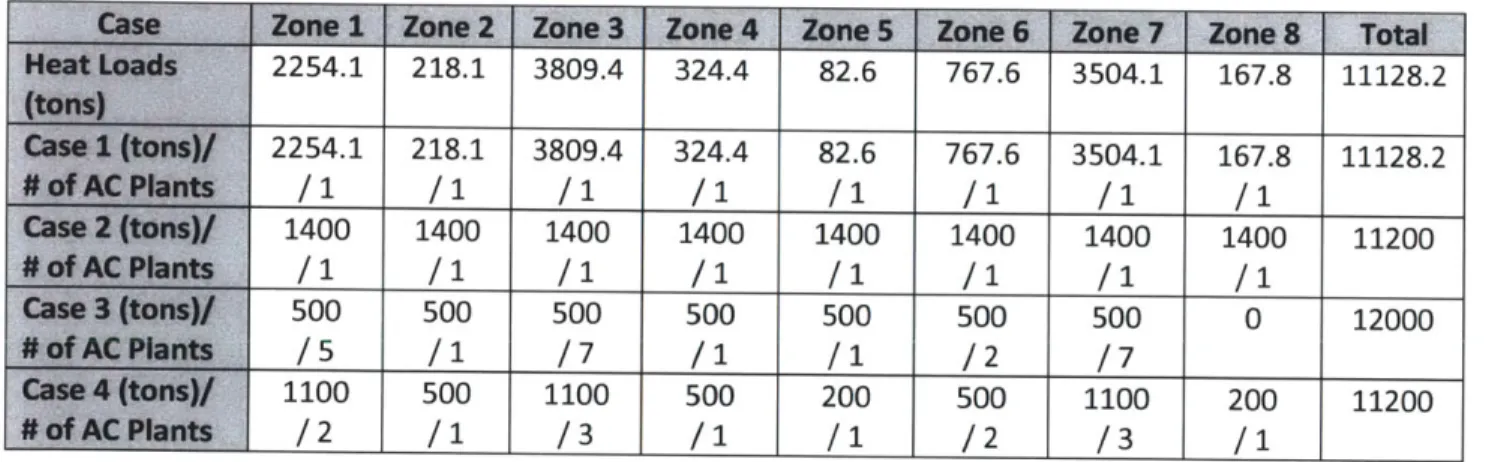
Within the design tool, the user has the ability to choose one of four different AC plant configurations:

1) have each zone create a custom size AC plant to match the heat loads produced within that

zone;

2) divide the total heat load by the number of zones and place one AC unit of that size in each zone;

3) create a standard size AC plant and place multiple numbers of that plant in each zone; and

4) manually enter AC plant capacities and number of coolers. An example of each of these cases is illustrated in Table 4 below.

2254.1 218.1 3809.4 324.4 82.6 767.6 3504.1 167.8 111Z8.Z 2254.1 218.1 3809.4 324.4 82.6 767.6 3504.1 167.8 11128.2 1400 1400 1400 1400 1400 1400 1400 1400 11200 500 500 500 500 500 500 500 0 12000 /5 /1 /7 /1 /1 /2 /7 1100 500 1100 500 200 500 1100 200 11200

A,

Table 4: Various configurations of AC plant capacities and numbers of plants

Since the plants can come in various and irregular sizes (especially with case 1), it was decided to use parametric scaling for the weights and dimensions of the plants. Additionally, since there is more than one type of AC plant, the dimensions and weights will vary based on the type of plant. The graphs below show the developed curves for the weights and dimensions of the two types of AC plants studied; "Type A" is based on current technology installed in Navy ships and "Type B" is a higher-efficiency model under development.

Weight vs. Capacity Type A

12

Length vs. Capacity Type A

14 13 -1 22 1 0.9 1 Caspsty Lttn/toni 1.4-1.4 -- tngth vs, Capacity Type A 0.407& 0 jitngh vv Cpadty Type A 0.7 0.9 1.1 Cap"1y t:oW/t0on

Width vs. Capacity

Type A

Width vs. Capacity Type B

1 00 -0 99 09 095 = -0.0264al -

0M-

Height vs. Capacity Type A

1 20 1.10 105 -1,00 1 00 0 261x 03518fm 1,2904 0.90 0.85 0.80 0.5 1 1 5 Casadty tmn/toi -eight capacity TypeA) 0698 0.696 0694 0.692 0690 0.682 0.684 0.682 0.680 0-671 y ~O.5075~.- 0A5SA it, I * 0.023~ta .0 6624 pL~ 05 07 0.9 11 1.3 15

Figure 4: Non-dimensionalized plots detailing how the AC plant parametrics, for the two types of plants, were determined

3 Values and types of plants were non-dimensionalized to ensure protection of proprietary data.

Page | 28

Weight vs. Capacity Type B

Weight Capadtv Type a -- *wnar woYght I(Apad"t 1A 15

Length vs. Capacity Type B

- ength Capadty Typea -thnear {langwth Capactv Type s) 13 1.5 -WIdthV-. Capacity Types Opadity Type s) 0.7 0.9 11 13 1.5

Height vs. Capacity Type B

- HeigWtvs

Capaity

The dimensions for the AC plants (determined from the Excel-created, trend-line equations above) can be exported to the Paramarine model in order to generate the visualizations and then assign those visualizations specific characteristics like weight with Paramarine's "char weight" variables.

The actual model currently only has "Type A" and "Type B" data; however, the model was built with the capacity to increase the number of types of AC plants up to 5; Appendix A has the directions on how to add in the data for the new types.

2.3 Pump Powering Comparison

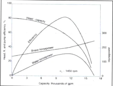
To select a pump for a system, there are three key characteristics which have to be decided on: pump capacity, pump head, and pump operating speed. Once these three characteristics are known, the system designer can use the series of pump curves (example seen in Figure 5) to choose the pump which operates most efficiently under that condition and determine how much power will be required to operate the pump.

fj*~ 300

1450

0 3' 6 9 12 18

Caaolf "oXsand of pm

Figure 5: Sample pump characteristic curve (Franzini, 1997)

While the tool was not designed to determine the optimal pump, it can help the user select a pump for the system.

As explained in section 2.2, the capacity for the pump can be calculated using the equation from the reference in section 2.1:

Qpm = 4.5 * T

where Qpm is the pump capacity (gpm) and T is the plant capacity (tons). (NAVSEA, 1987)

By the user entering in the locations of the loads and the locations of the zones, the tool will determine

identical," (NAVSEA, 1987) the zone with the highest heat load (and therefore highest capacity requirement) will drive the pump capacity characteristic. By utilizing the same pump across the ship, one pump will not overpower another "dead-heading" the flow, purchasing and maintenance costs can

be reduced, the number of repair parts maintained on board can be lessened, and training for the pumps can be standardized.

The second characteristic to be calculated is the amount of head loss (hL) that the pump has to overcome; hL is the fluid-friction energy loss per unit weight of fluid. The sources of this "fluid-friction" come not only from the resistance of flow as it travels down the length of pipe, but also from the resistance caused by direction changes, transition to different pipe sizes, etc. The determination of the total hL can be calculated from Bernoulli's equation (Franzini, 1997):

P1 V71

P

V2

-+ z1+-= -+ z2 +-+ hL

y 2g y 2g

where P is pressure, y is specific weight, z is the vertical height, V is fluid velocity, g is acceleration due to gravity, and hL is the total head loss which can be calculated by summing up the individual sources of hL:

hL = _X hL(X)

where hL(x) is each of the individual sources. The derivation of the values for the individual sources will be discussed below.

The first contributor to the total head loss was the head loss due to friction along the length of the pipe. To calculate this value, the following equation was utilized (Crane Co, 1982):

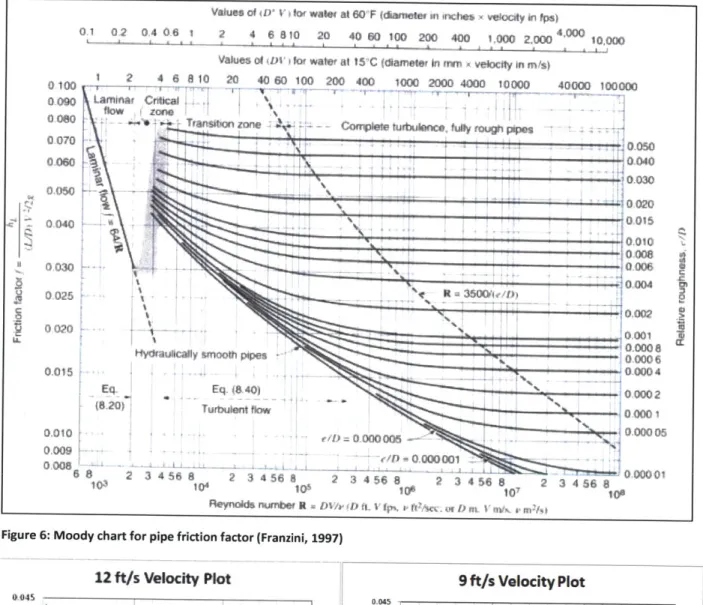
L * V2

hL (1)* _2g

where hL(1) is the head loss due to friction along the length of the pipe,

f

Thef value can be determined by one of the two primary means: mathematically or via extraction from the Moody diagram shown in Figure 6. Assuming turbulent flow through the pipe, the following equation derived from E. Haaland's equation can be used to solve forf (Franzini, 1997):

1.63639

(

inR - 1.45 225)

where e is the absolute roughness factor and R is the Reynolds number:

LV

R

Due to the complexity of this equation, for the standardized maximum velocity cases of 9 fps and 12 fps, thef value was determined using the Moody chart.

Several decisions had to be made about the pipes and flows to obtain the friction factor,

regardless of using the equation or the chart. The first was deciding on a value for e. The value selected was 0.046mm, as this is the absolute roughness for welded-steel pipe. While the Navy uses Ni-Cu piping

(e = .0015mm for drawn tubing and copper), the piping segments are welded together, hence the use of

the higher value. To calculate the R, pipe diameter, flow velocity, and viscosity have to be identified. As further discussed in section 3.1.4, the program is currently designed for freshwater, so kinematic

viscosity is taken to be 1.00E-06 m2_{/s; the diameters for the headers and branches were calculated per} section 2.1.

Per the NAVSEA design criteria manual, "All chilled water piping is to be designed so that the water velocity does not exceed 12 feet per second in the mains, cross connections, and risers, and 9 feet per second in the branches." (NAVSEA, 1987). The equations for the values off are a curve fit of the data in Figure 7, extracted from Figure 6 for the specific design problem:

Values of 4D' * ior wate& at60'F (darnter Kn nches . velocty in ps)

01 0 2 OA 0 6 1 2 4 6 810 20 40 60 100 200 400 1,000 2,000 4,000 10,000

I,

-. - I .--

-Values of 01X for water at 5"C (diameter In mm . welocity In m/s)

1 2 4 6 8 10 20 40 60 100 20)0 400 1000 2000 4000 10000 40000 100000 0 100

0- Lamiorlf Crtic-al

080 - sasor ine4kspe turbt*Ac tilty mogh 11p0"

0 000ct sot pps- 00 000004 00 0050 Eq E. 0440 0000 0.010 0.010 0.000 58 2 3468 10 2 34 680 2 456800 20 4568 200 40000

car ie fraon f facon ztinfu9g7)CFrno

10 0-000 Eq- Eq ($,40)0 006 Turbulnt no 0040 R~ 355 .00 0.010 e/ 0.0.001 D.009 0,0.000 0008~ 0000 10 1041101%0 1000100110

0knoi 006r = Aft Vpv r k 1fi - i 000

Fiur 6: 2od 3hr 45o 8 2ip 3rcto 45cto 8F i 219 469734) 8 234

12 ft/s Velocity Plot 9 ft/s Ve 4)045 0.045 oeas -S0.0s 004s 0.03 0025 0 0e00 0 022 1015 0.01 ocese0.00s 0005 0 0 000 0.OOE+00 2.OOE+05

000-00 50E+5 iO00&04 S 50-06 Reyn

Reyn.SA Number 1)

Figure 7: Plots obtained from pulling points from the Moody Diagram at a) 12 fps and b) 9 fps.

locity Plot

4.00E+05

olds Number (R)

f

f9ft/s = .4025 * -. 247

To determine the L value, several assumptions had to be made. It was assumed that the length was broken up into the X, Y, and Z directions. The length in the X direction is the distance from the

Page 1 32

center of the HX to the X location of the load. It was also assumed that the length the fluid travels down in this direction is all in the main header. The length in the Y direction is the distance from the header to the Y location of the load; the length in the z direction is the distance from the header height to which the load is connected (port or stbd) to the z location of the load. As the distances traveled in the Y and Z directions were taken to be in the branch piping, their lengths could be combined and were paired with the same

f

The flow velocity value and diameter were calculated via the equations discussed in section 2.1.1.

The remaining contributing factors to hL were determined using the following equation (Franzini,

1997):

hL (X) -

k7V

where k was selected from Table 5 or selected as discussed below. The following assumptions were made to determine how much head loss the remaining contributing factors would contribute:

1) Isolation valves: the assumptions were made that there were 6 isolation globe valves (one at the

inlet and outlet of the AC plant, one at the inlet and outlet of the pump, and one at the inlet and outlet of the supply and return branch lines to the applicable load).

Fiting k

Gilohe Valve. wide open 1if

Angle salve. wide open

(lose-iretum end 2.

T, through side outlet 1.8

Short-radius elbow 0

Medtum radmau eihow 0.75

Long-radius elbow 0.60

4Y clbow 0.42

Gate valve, wide open 0.19

half open ).06

Table 5: Values of loss factors for pipe fittings (Franzini, 1997)

2) Entrance loss coefficient: in transitioning from the header to the branch line (square edged mating), a k value of 0.5 was selected (from Figure 8).

Figure 8: Entrance loss coefficients (Franzini, 1997)

3) Bends in the piping: short-radius elbows were assumed to exist as the branch piping

transitioned from the y direction to the z direction; if the load was at the same height as the header, no bend was considered to exist.

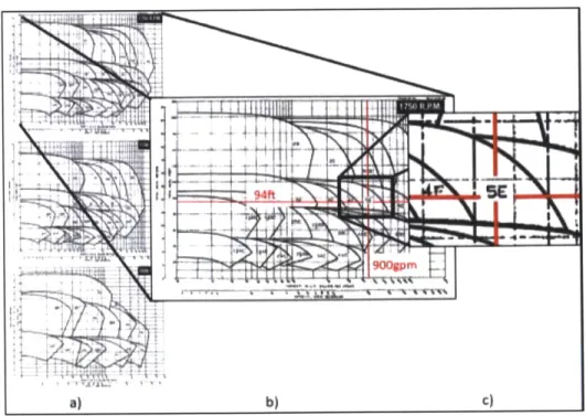
With uncertainty as to the value of the third factor (pump speed), and the unlimited variability in head and capacity combinations as zone size varies, it was decided to end the program's search for pumps at this point. A specific example of why is detailed as follows: for one specific zonal configuration (four zones), it was determined that required pump capacity was 900gpm and head to be overcome was 94ft. To select a pump and determine its characteristics, the following process was worked through:

1) Identify a specific pump meeting these requirements. Fortunately, Bell and Gossett provided

the following charts for their 1510 Series pumps, which made this possible:

Figure 9, a) Pump head and capacity as a function of speed: Top = 1750 RPM, Middle = 1150 RPM, Bottom = 3500 RPM; b) Expanded 1750 RPM plot with the provided conditions highlighted in red; c) expanded plot of the pump which meets the needs of the system. (ITT Industries: Bell & Gossett, 1998)

2) Determine the specifications of the pump chosen. As illustrated below, there are variations of the Series 1510 5E based on the impeller diameter.

MCARTY IN U.9, QALLONS PEA MINUTE

Figure 10, Pump curves for the 1510 Series 5E pump at 1750 RPM. The red lines indicate the requirements for the designed condition (ITT Industries: Bell & Gossett,

1998)

To ensure the requirements can be met, the 10.5" diameter pump is selected.

3) Extract the data for the given pump. Once the pump has been selected, power and efficiency

can be obtained from the curve. One key note is that weight data is not provided; to obtain weight data, the manufacturer must be contacted. Weight was provided as a function of the power required for the

pump and is given in two separate components: 1) weight of the pump structure and impeller and 2) weight of the motor. The table detailing this is shown below.

Tb 425 225 650 20 240 665 25 45 260 695 30 -42075 40 445 510 955 50 520 965

Table 6, Weights for the Series 1510 5E pump (ITT Industries: Bell & Gossett, 1998)

An automated system was set up within the CSDT to determine the impeller diameter, power, efficiency, and weight for the Series 1510 5E pump. However, if the zonal configuration is changed to five smaller zones (from the four in the example above): 1) required pump capacity will decrease as chilled water capacity per zone decreases and 2) required head will decrease as a function of speed (which is a function of capacity) squared. Therefore, the new requirements will most likely be outside of the boundaries of the 5E pump.

To try and account for all reasonable capacity and head variations (for the Series 1510 pumps alone) would require the tabular conversion of over 1000 plots; as an alternative to selecting a specific pump, the following assumptions and analyses were developed:

* The head loss and capacity can be translated into the amount of brake power (kW) the pump requires by using the following equation (Franzini, 1997):

Power (kW) = y

Q

1000 *

where y is the unit weight of the fluid, Q is the CSDT determined rate of flow, and h is the CSDT determined head loss. An assumed value of 80% efficiency, j7, was selected. While efficiency will vary based on the pump's characteristics, it was assumed that an optimum pump would be selected for the given plant; from Figure 11 and using data from the Series 1510 pumps, the