HAL Id: hal-02383505
https://hal.archives-ouvertes.fr/hal-02383505
Submitted on 27 Nov 2019HAL is a multi-disciplinary open access archive for the deposit and dissemination of sci-entific research documents, whether they are pub-lished or not. The documents may come from teaching and research institutions in France or abroad, or from public or private research centers.
L’archive ouverte pluridisciplinaire HAL, est destinée au dépôt et à la diffusion de documents scientifiques de niveau recherche, publiés ou non, émanant des établissements d’enseignement et de recherche français ou étrangers, des laboratoires publics ou privés.
Energy efficiency drives the global seasonal distribution
of birds
Marius Somveille, Ana S.L. Rodrigues, Andrea Manica
To cite this version:
Marius Somveille, Ana S.L. Rodrigues, Andrea Manica. Energy efficiency drives the global seasonal distribution of birds. Nature Ecology & Evolution, Nature, 2018, 2 (6), pp.962-969. �10.1038/s41559-018-0556-9�. �hal-02383505�
Energy efficiency drives the global seasonal distribution of birds
Marius Somveille1,2,3*, Ana S. L. Rodrigues3, Andrea Manica2
1Edward Grey Institute, Department of Zoology, University of Oxford, United Kingdom
2Department of Zoology, University of Cambridge, United Kingdom
3Centre d’Ecologie Fonctionnelle et Evolutive CEFE UMR 5175, CNRS - Université de
Montpellier - Université Paul-Valéry Montpellier – EPHE, France *Correspondence to: [email protected]
The uneven distribution of biodiversity on Earth is one of the most general and puzzling patterns in ecology. Many hypotheses have been proposed to explain it, based for example on evolutionary processes or constraints related to geography and energy. However, previous studies investigating these hypotheses have been mainly descriptive as controlled experiments are hardly feasible at such large geographical scale. Here, we use bird migration – the seasonal redistribution of about 15% of bird species across the world – as a natural experiment for testing the species-energy relationship, the hypothesis that animal diversity is driven by energetic constraints. We develop a mechanistic model of bird distributions across the world and across seasons based on simple ecological and energetic principles. Using this model, we show that bird species distribute as to optimise the balance between energy acquisition and energy expenditure while taking into account competition with other species. These findings support, and provide a mechanistic explanation for, the species-energy relationship. They also provide a general explanation of migration as a mechanism allowing birds to optimise their energy budget in the face of seasonality and competition. Finally, our mechanistic model provides a tool for predicting how ecosystems will respond to global anthropogenic change.
One of the most promising hypotheses to explain the global distribution of biodiversity is the species-energy relationship, which states that the constraints of energy supply and demand drive animal diversity1,2. In particular, according to Lotka’s maximum power principle3, natural selection should favour organisms that have the most favourable balance between the energetic costs associated with their environment and behaviour and the benefits in terms of
access to available energy to fuel metabolism4. Accordingly, energy-efficiency has been
shown to affect the movement behaviour and spatial distribution of species as they optimise energy acquisition6,7. Species, however, do not exist in isolation: the energy-efficiency of a particular distribution depends not only on the quantity of available resources, but also on the distribution of the other species competing for the same resources. Overall, this should translate into an energy-efficient distribution of all species across the world, in which each species minimises its energy expenditure while targeting areas with maximum energy available given the distribution of the other species. Macroecology has provided support for this hypothesis, with studies revealing a positive and linear relationship between species richness and the amount of available energy in the environment8,9. However, these studies
were mainly descriptive (e.g. 10) and a mechanistic understanding of this relationship has thus
far proven elusive.
Birds are highly mobile organisms, and twice a year about 15% of species migrate between breeding and non-breeding grounds11, in a “seasonal ecological adjustment on a gigantic
scale”12. Bird migration thus provides a natural experiment for testing hypotheses about the
mechanisms driving the spatial distribution of species13,14, as any such mechanisms must explain not only spatial patterns of bird diversity but also the seasonal redistribution of such diversity. Previous macroecological studies of bird migration support the hypothesis that energy drives the seasonal distribution of migratory species15,16, pointing to negative costs associated with winter harshness and longer migratory distances, as well as to benefits in terms of access to seasonally available resources16. These studies, however, only consider migratory species, are correlative, and integrate energy implicitly rather than explicitly. Here, we present a mechanistic model of the geographical distribution of all terrestrial bird species across the world and throughout the year that explicitly integrates energy, by expressing costs and benefits into a common energetic currency and by accounting for inter-specific competition. Built from first ecological and energetic principles, our spatially-explicit model
simulates a virtual world in which species are distributed in an energy-efficient way. By comparing model outputs to empirical global patterns of bird diversity16,17, we test the prediction that energy-efficiency drives the distribution of birds across space and seasons.
Results
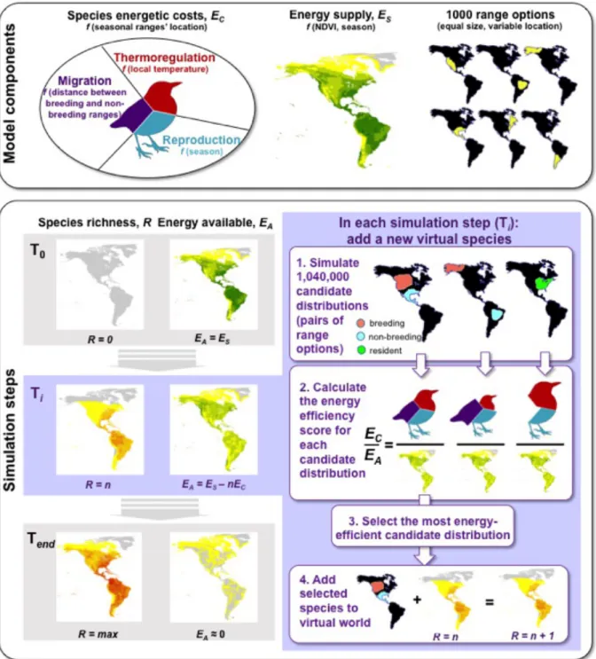
Our model is built from the assumptions that the energetic costs associated with any given species’ distribution comprise thermoregulation costs, reproduction costs, and migration costs (in addition to a basal energy use for existence, constant across species) whereas energy supply available to a species at any given season is a function of the primary productivity available and not yet appropriated by other species. Each model simulation starts with a virtual empty world with the same geography and seasonality as the real world (similar landmass distribution, similar climate, similar primary productivity, and with two seasons), which is then progressively filled with virtual bird species. We have not incorporated in the model any inter-specific variation in morphology, physiology or biology, thus assuming ecological, demographic and energetic equivalence between these virtual species. In each simulation step, a single new species is added, selected as being the most energy-efficient among many candidates (i.e., the one whose combination of breeding and non-breeding range results in the most favourable costs-benefits balance), and the energy supply in the virtual world is depleted accordingly. New virtual species are added until the virtual world becomes nearly saturated (see Methods and Fig. 1 for more details). The model has four free parameters (three associated with the energetic costs of migration, thermoregulation and reproduction, and one associated with the scaling of energy supply; see Methods and Supplementary Figure 1). For any combination of parameter values, a virtual world saturated with virtual species is deterministically simulated, from which five geographical patterns representing the global seasonal distribution of birds can be derived and contrasted with
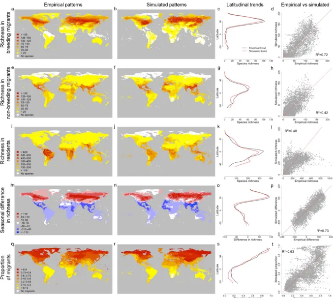
observations. We found the parameter values that best predict the empirical patterns (i.e., the best-fit model) using a genetic algorithm (see Methods and Supplementary Information). We found that the best-fit model is able to predict very well all five empirical patterns (Fig. 2;
R2 from 0.42 to 0.73). Indeed, it captures the fact that the bulk of breeding migrants occur in
the northern Hemisphere around 50°N (Fig. 2a-d) and redistribute for the non-breeding season to the southern part of the northern Hemisphere, with few species crossing the equator (Fig. 2e-h). It predicts well the peak in resident bird species in the tropics (Fig. 2i-l). It also captures a peculiarity in the global pattern of bird migration17: the transition from avian communities that are net senders and those that are net receivers of breeding migrants at around 35°N, a band of high species turnover with similar richness in both seasons (Fig. 2m-p). Finally, the model accurately predicts the latitudinal increase in proportion of migrants from the equator to the poles (Fig. 2q-t). Overall, the model captures very well the strong asymmetry between the northern and southern hemispheres when it comes to patterns in bird diversity (Fig. 2; 17).
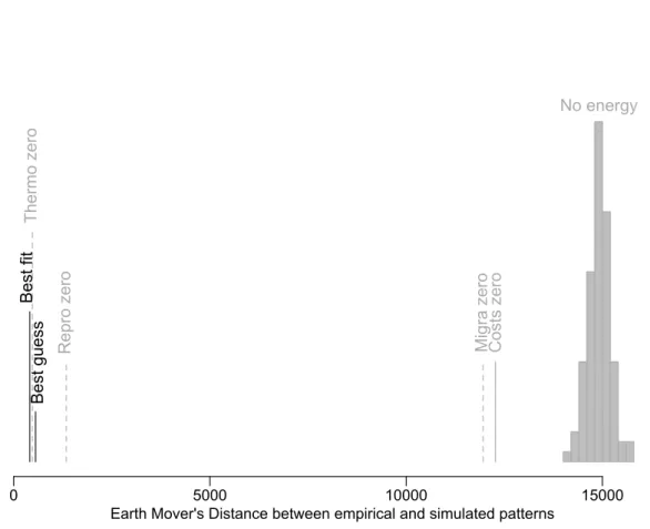
To assess the significance of our model’s predictive ability, we contrasted it with a null model that does not take into account energetic constraints, which fails to predict any of the empirical patterns (Figs. 3 and 4 and Supplementary Figure 3, all R2 negative), and is significantly outperformed by the best-fit model (Fig. 4; p < 0.001). A null model in which energetic costs (i.e. migration, thermoregulation and reproduction) are all set to zero (thus driven by energy availability only) also failed to produce realistic patterns (Figs. 3 and 4 and Supplementary Figure 4, all R2 negative). These results thus confirm that energy-efficiency (i.e., the optimisation of the balance between energy acquisition and energy expenditure) is the key mechanism underpinning the good predictive ability in our model, rather than simply energy supply. To assess the relative importance of the three components of energetic costs in driving the model outputs, we also tested null models whereby each of the components were
removed in turn. When either migration or reproduction costs were set to zero, the model was no longer capable of producing realistic patterns (Figs. 3 and 4, and Supplementary Figures 5 and 6), indicating that each of these components is crucial to understanding empirical patterns. In contrast, removing thermoregulation alone had relatively little effect on model performance (Figs. 3 and 4 and Supplementary Figure 7), suggesting this component is less important. This could be due to the fact that cold climate is highly correlated with low resource availability and therefore does not add much to the explanatory power of the model whose output is already strongly driven by the geographical and seasonal variation in energy supply. In fact, including thermoregulation improves predictions in temperate areas with some relative mismatch between winter NDVI (being relatively high) and winter temperature (being below the thermo-neutral zone of species). It helps better predict the distribution of species during the winter in these temperate environments (e.g. North America, Europe, East Asia) and consequently also the latitudinal peak in breeding migrants (further southwards; see Fig. 2 versus Supplementary Figure 7).
Further confirmation that our model realistically captures biological processes comes from the fact that the best-fit parameter values (obtained by fitting the full model to the empirical data) are very close to values estimated independently from the literature (Supplementary Figure 8; Supplementary Information). The best-guess model based on the latter set of parameter values also has excellent predictive ability, even if not as good as the overall best-fit model (Fig. 4 and Supplementary Figure 9), and deviations between the two are plausible given the data (Supplementary Information). Removing thermoregulation cost from the model also leads to parameter estimations that are realistic but not when migration or reproduction costs were set to zero (Supplementary Figure 8).
Overall, the strong ability of our mechanistic model to predict macroecological patterns of bird diversity suggests that it successfully integrates the main costs and benefits affecting the global geographical distribution of terrestrial bird species, and provides strong support to the hypothesis that these distributions are driven by energy-efficiency.
The mismatches between the empirical patterns and those predicted by the full best-fit model are informative. In particular, the model tends to under-predict richness in migrants in open habitat regions (e.g. western half of North America, central Asia, East Africa) while over-predicting it in regions dominated by forest (e.g. eastern half of North America, central and eastern Europe, south-east Asia; Supplementary Figure 10). This may reflect limitations of using NDVI as a proxy for locally available energy across different types of habitat. The model also under-predict richness in resident species in major mountainous regions, mainly the Andes and the Himalayas (Supplementary Figure 10c), which likely reflects processes not taken into account in this study such as the effect of habitat and topographic heterogeneity on speciation rate, range size and endemism18–21 in these regions. This is also what is likely affecting the fact that the model generates fewer virtual species than the empirical total number of species (7783 species for the full best-fit model; 7844 for the best-guess model; 9356 for the empirical model), as this is most likely due to the model not being able to capture the high number of small-ranged, endemic species in areas with high habitat and topographic heterogeneity.
Our analysis provides a unified mechanistic explanation of bird migration as a behaviour that allows highly mobile avian species to optimise their energy budget in the face of fluctuating resources and inter-specific competition. Indeed, in the early parts of the simulation, virtual species are resident in the tropics (Supplementary Figure 11a), which is consistent with Fretwell’s prediction that a bird “in a totally noncompetitive atmosphere, might find itself a
competition reduces local energy supply, making it more energetically efficient to migrate to areas with unexploited seasonal surpluses of energy. In our increasingly crowded virtual world, species progressively start exploiting more extreme pockets of seasonally available energy supply, often migrating longer distances (Supplementary Figure 11b). Our results confirm the important role of the competitive reduction of energy supply, which has been
proposed to be a key driver of bird migration22–24, in shaping the distribution of migrant and
resident bird species across the world and over the year.
Whilst we focused on terrestrial birds, we expect our model to be directly transferable to other highly mobile taxa, such as oceanic fish or cetaceans. Its application to taxa requiring specific habitats during their life-cycle (e.g., cliffs for seabirds, caves for bats) would require integrating the distribution of such resources when considering possible distributions for virtual species. The principles of the model are more broadly applicable even to low-mobility taxa, such as amphibians, or even non-mobile taxa, such as plants, by assuming migration is too costly or impossible, such that only resident distributions are energetically efficient. These species have other mechanisms for dealing with seasonality, such as dormancy or hibernation, which could be easily added to our model by assuming different energetic requirements in different seasons.
A mechanistic explanation of how species distribute across the world is key to improving our capacity for predicting how ecosystems will respond to global change. Effects of climate change on temperature and precipitation25 are already affecting thermoregulation costs and the distribution of energy supply. Anthropogenic land-use changes are increasing competition in areas where humans appropriate larger portions of the energy supply (e.g., through agriculture and urbanisation26), but also increasing resource supply in others (e.g., in landfills27). Our mechanistic model provides a useful tool for making predictions of such effects on biodiversity under various scenarios of global change.
METHODS
Empirical bird data. Spatial polygons representing the global distribution of 9783
non-marine bird species were obtained from BirdLife International and NatureServe28. The data and their treatment are described in detail in 17. Briefly, range maps were converted into
presences and absences on a global grid of equal-area (~23,322 km2), equal-shape hexagons29,
with 7352 hexagons remaining after removing the ones that contained no land and for which not all environmental data were available. After removing the species for which the seasonal geographical distributions did not overlap with any remaining land hexagons, 9356 species remained for the analysis (species occuring in both the western and eastern Hemispheres were treated for analytical purposes as two species). Migratory species were defined as those whose breeding and non-breeding distributions did not completely overlap, totalling 1403 species. From these data, we generated five spatial patterns, capturing the global seasonal distribution of terrestrial birds: richness in breeding migrants: number of species present in each hexagon only during their breeding season; richness in non-breeding migrants: number of species present in each hexagon only during their non-breeding season; richness in residents: number of bird species present in each hexagon year-round; seasonal difference in richness: number of breeding migrants minus number of non-breeding migrants; proportion of migrants: number of migrant bird species (both breeding and non-breeding visitors), divided by the total number of bird species (both residents and migrants).
Virtual worlds. The virtual worlds we simulated have the same geography and seasonality as
the real world: a similar landmass distribution, mapped onto the same hexagonal grid as above; two seasons, corresponding to the northern summer (April to September) and northern winter (October to March); similar climate, as measured by temperature and precipitation; and similar resources, as measured by the Normalized Difference Vegetation Index, NDVI. Since
no migratory flyways cross the Atlantic or the Pacific Oceans, simulations were run separately for the western Hemisphere (WH < 30°W) and for the eastern Hemisphere (EH > 30°W). Temperature and precipitation were computed for each hexagon in each season as the
average across the corresponding six months using data from WorldClim at resolution 5’ 30.
Monthly estimates of NDVI were obtained from NASA’s Earth Observatory at a resolution of
0.1° 31; pre-processed as in 16, summed across the six months of each season and averaged for
the pixels in each hexagon to obtain local seasonal NDVI values.
Virtual bird species. Each virtual species inhabits a particular combination of a breeding
range and a non-breeding range, either congruent (resident species) or different (migratory species). Each range is composed of multiple local populations (one per hexagon); a single hexagon may have populations of several species. We assumed all species are functionally equivalent (ignoring differences in traits and ecology), that all populations of all species are the same in their basal energy use for existence (thus assuming energetic equivalence between bird species32–34), and that individuals are homogeneously distributed within each species’ range. We thus modelled an average species: with a body mass (M) of 38.6g (median among empirical values in 35); with an average geographical range size of 131 hexagons if in the WH, 180 hexagons if in the EH (median values in our empirical dataset).
Model overview. The SEDS (Seasonally Explicit Distributions Simulator) model is a
mechanistic model of the geographical distribution of bird species across the world and throughout the year, built from first ecological and energetics principles, relating the energy supply available in the environment with the energy requirements of bird species. It is a costs-benefits model whose common currency is energy, built from three main components: a module estimating the costs associated with species’ energy requirements; a module estimating the spatial and seasonal variation in energy supply; and a module simulating virtual species’ geographical range options. Integrating these three components, the model is
applied through a sequence of simulation steps whereby a virtual world is progressively filled with virtual species until it becomes saturated (Fig. 1). Our model is not an evolutionary model of competition, neither taking into account the potential mortality associated with the processes nor the potential increases in reproductive output under favourable conditions, essentially assuming species’ populations to be at demographic equilibrium.
Energetic costs. For each local bird population, the energetic requirements were composed of
the basal energy use for existence, BEU, which was set to be 1 (arbitrary) unit, and additional
costs associated with migration (mc), thermoregulation (tc) and reproduction (rc), which were
converted into such arbitrary units of energy use (Supplementary Figure 1).
The cost of migration, 𝑚!, corresponds to the energetic cost of, each year, travelling twice
between the breeding and non-breeding ranges. We assumed that: 𝑚! increases linearly with
distance travelled (thus 𝑚! = 0 for resident species); migration happens instantaneously at the end of each season (its cost added to the corresponding season to reflect the previous investment in fat reserves). For each season, 𝑚! was computed as a function of the great circle distance, dm, between the centroids of the breeding and non-breeding geographical
ranges (average distance travelled by individual birds of the species assuming that they
migrate using the shortest route). Thus 𝑚! = 𝛼 ∗ 𝑑!, with α a free parameter determining the
energetic requirements for a bird to travel a unit of distance (Supplementary Figure 1).
The cost of thermoregulation, 𝑡!, corresponds to the additional energetic cost of maintaining a
relatively constant internal body temperature for endotherms like birds. Empirical and theoretical studies indicate that species have a thermo-neutral zone, a range of environmental temperatures (between a lower critical temperature TLC and the upper critical temperature
TUC) within which 𝑡! = 0, and outside of which costs increase linearly36,37. We ignored the
increase in energy demand above TUC, since it has been poorly quantified previously and only
TUC (34.3°C) of 167 species sampled across the bird phylogeny and the world38. We therefore
focused on the thermoregulation costs when the ambient temperature is below TLC. The
Scholander-Irving model of heat transfer39 describes how body temperature is regulated by balancing the rates of heat production and heat loss. Its core equation for a resting (endotherm) animal with minimal heat loss (by maximising insulation and optimising body
posture) is 𝑇!− 𝑇!" = 𝐵𝑀𝑅/𝐶, where Tb is the body temperature (40°C for birds), BMR is
the basal metabolic rate in mlO2/h, and C is the rate of heat loss or thermal conductance. The
lower critical temperature of the thermo-neutral zone can therefore be obtained as 𝑇!" = 40 −
𝐵𝑀𝑅/𝐶. We assumed that if the ambient temperature (Ta, in °C) is below TLC, the cost of
thermoregulation increases linearly with the temperature difference between TLC and Ta such
that 𝑡! = (𝐶 𝐵𝑀𝑅) × (𝑇!"− 𝑇!) (Supplementary Figure 1). So, if 𝛽 = 𝐵𝑀𝑅/𝐶, the cost of
thermoregulation for a virtual species in a focal season was computed as a function of the
ambient temperature with a free parameter β, as: 𝑡! =
!"! !!!!
! ,𝑖𝑓 𝑇𝑎< 40 − 𝛽 0 ,𝑖𝑓 𝑇𝑎 ≥ 40 − 𝛽
.
The cost of reproduction, 𝑟!, corresponds to the extra energy requirements for the production
of new organisms. We assumed this is all incurred in the breeding season, modelling it as a fraction of the basal energy use for existence, with free parameter 𝛾, as: 𝑟! = 𝛾 ∗ 𝐵𝐸! (Supplementary Figure 1).
For any local bird population i of a given species at a given season, the energetic costs were computed as: 𝐸!"!" = 1 + 𝑚!+ 𝑡!" + 𝑟! (for the breeding season) and 𝐸!"!" = 1 + 𝑚!+ 𝑡!" (for the non-breeding season), determined by the three free parameters (α, β, γ). The total energetic cost for a species at a given season was then computed as the mean of the energetic costs of the p local populations across the seasonal ranges, i.e. 𝐸!!" = !!!!𝐸!"!" 𝑝 (for the breeding season) and 𝐸!!" = !!!!𝐸!"!" 𝑝 (for the non-breeding season).
Energy supply. In each hexagon, energy supply, ES, is the total amount of resources that is
used to fuel bird species’ metabolism. We modelled ES as proportional to NDVI, a
remote-sensing measure of greenness that correlates well with primary productivity (often used in macroecological studies analysing the effect of the availability of energy and resources on the distribution of bird diversity14–16,40–42). NDVI varies across space (hexagons) and between seasons. We assumed that, in any given hexagon j, the higher the NDVI the higher its carrying capacity for birds, such that 𝐸!" = 𝜇 ∗ 𝑁𝐷𝑉𝐼!, with µ a fourth free parameter of the model. This parameter was used for adjusting the energy supply (i.e., acting as carrying capacity) in order for the model to generate a realistic total number of virtual species (i.e. similar to the empirical number). The energy available, 𝐸!", is equal to the energy supply minus the energy already consumed by species previously simulated and occurring in hexagon j. The energy available to a species at a given season was computed as the mean of the energy available in the p hexagons across the seasonal range, i.e. 𝐸!!" = !!!!𝐸!"!" 𝑝 (for the breeding season) and 𝐸!!" = 𝐸!"!"
!
!!! 𝑝 (for the non-breeding season).
Virtual species’ range options. We generated 1000 contiguous geographical ranges in our
virtual world (400 in the WH, 600 in the EH, reflecting differences in area) to serve as options from which the distributions of virtual species were simulated (Fig. 1). Ranges were generated using a method adapted from the spreading dye algorithm43,44 through a climate-driven approach of range expansion that has been shown to capture well the empirical
distribution of bird ranges shape45. Each range was seeded from a single randomly selected
hexagon and then allowed to stochastically spread into adjacent unoccupied hexagons, constrained by climatic conditions, until reaching a fixed size. For each range, an initial climatic optimum was obtained from the position of the seed hexagon in a climatic space defined by mean annual temperature standardised) and mean annual precipitation (z-standardised after being log-transformed). We then selected two neighbours of the seed
hexagon, with the probability of selection being higher for neighbours closer to the climatic optimum (i.e. lower Euclidian distance d in climatic space between itself and the climate
optimum), calculated as 2(d+1)-30, divided by the sum of these values across all neighbours
(hence decaying exponentially with increasing climatic distance d). We then repeated this procedure, each time redefining the climatic optimum as the average climatic condition across the already selected (i.e., occupied) hexagons and selecting 25% (rounded to the larger integer) of the set of unoccupied neighbours of the occupied hexagons (summing the probabilities of the ones being neighbours of more than one occupied hexagon), until the
desired range size was reached (131 hexagons, ~3.05 million km2, in the WH, 180 hexagons,
~4.20 million km2, in the EH).
Simulation steps. Each simulation is performed on the WH and EH separately. At the start of
the simulation (T0), the virtual world is empty of bird species and the energy available (EA) in
each hexagon is equal to the energy supply (ES) in each season (Fig. 1). Then, each simulation
step consisted of four sub-steps:
• Sub-step 1: generate candidate virtual species by combining all possible pairs of range options, each option occupied in either the breeding season or in the non-breeding season, and each species breeding in either the northern summer or the northern winter. There are thus 320,000 candidate virtual species (from 400 range option) in the WH and 720,000 (from 600 range options) in the EH. This sub-step only needs to be performed once: the same set of candidate virtual species is used in all steps of the simulation.
• Sub-step 2: for each candidate distribution, compute a year-round energy-efficiency score (E) defined as energetic cost divided by energy available, combined for both seasons, such that 𝐸 =!!!!"
!!" +
!!!"
!!!"
The costs for each candidate species depend on its spatial location: thermoregulation costs are higher in cooler regions and migration costs relate to the distance between breeding and
non-breeding ranges. Reproduction costs are allocated only to the non-breeding range. Energy available also varies with spatial location, depending on the initial energy supply (NDVI) as well as how much of it has been appropriated by previously simulated species.
• Sub-step 3: the virtual species selected is the one with the lowest E (the most energy-efficient).
• Sub-step 4: the newly simulated virtual species consumes energy within its seasonal geographical ranges equivalent to its corresponding energetic cost, effectively depleting the energy available in all the hexagons across its geographical distribution as: 𝐸!!"− 𝐸!!"
across the breeding range and 𝐸!!"− 𝐸!!" across the non-breeding range.
The simulation then proceeds, each step going through sub-steps 2, 3 and 4 to add a new virtual species.
The SEDS model therefore assumes that the scarcer the energy supply and the higher the number of other species competing for it, the harder (and thus less energy-efficient) it is to
access it. Biologically, this may correspond to costs associated with mutual interference46,47,
increasing search time48, and territorial defense49. As energy-efficiency is higher when the difference between energetic costs and energy available is higher, it may be more energy efficient to occupy a geographical area with low resources and low competition than a crowded highly productive area. For example, taking a species with an average energetic cost of 1.5 units across its geographical range, if no other species are present, a geographical range in rain forest (average energy supply = 200, so energy-efficiency score = 0.0075) is more energy-efficient than a range in desert (average energy supply = 30, so energy-efficiency score = 0.0500). But if the rain forest is already crowded with other (previously simulated) species using 90% of the energy supply (available energy supply = 20, so energy-efficiency score = 0.075), then the desert without competitors is a better option. Energy supply therefore acts as a carrying capacity that limits the number of populations of different species that can
co-occur in any given hexagon. We stopped simulating species when 95% of the energy supply in at least one season across the world was used, i.e., when the virtual world was nearly saturated with simulated species.
Parameter fitting: best-fit model. The SEDS model contains four free parameters: α, β, γ,
and µ. For any combination of parameter values, a virtual world saturated with virtual species can be deterministically simulated, from which it is possible to map each of the above-described global spatial patterns. We searched the four-dimensional parameter space for the combination of parameter values that best fit the empirical data, i.e., that produces a virtual world in which the three basic patterns – richness in breeding migrants, richness in non-breeding migrants, richness in residents (the other two patterns being derived from combinations of these) – best match the empirical patterns. We computed the Earth Mover’s
Distance50 to quantify the similarity between simulated and empirical spatial patterns, which
is a measure of goodness-of-fit that is also sensitive to the number of virtual species allowed in the virtual world, and a genetic algorithm to fit the parameters (see Supplementary Information for details; results in Fig. 2).
Parameter estimating: best-guess model. For each of the four free parameters, we also
obtained coarse estimates from the literature, wholly independent from the dataset we used (see Supplementary Information for details; results in Supplementary Figure 8). We contrasted these with the parameters obtained from the fitting process to evaluate the biological realism of the latter.
Null models. We tested whether our model based on energy-efficiency produced significantly
better results than expected by comparing its results to simulations under each of several null models (Figs. 3 and 4):
1. A null model without integration of energetic considerations (called no energy). As in the SEDS model, the simulation starts with a virtual world empty of species, but then
the geographical distribution of the virtual species added in each step is selected at random among all the candidates, irrespective of energetic costs or energy supply. For each of 100 runs of this null model, we generated 3886 virtual species for the WH and 5206 virtual species for the EH, corresponding to the numbers in our empirical dataset.
2. A model in which the distribution of species is purely driven by energy supply, without taking into account costs (other than basal requirements for existence; called
costs zero). Here, we set costs of migration, thermoregulation and reproduction to 0 by
using the following parameter values: α = 0, β = 80, γ = 0. As in the SEDS model, the simulation starts with a virtual world empty of species where the energy available is equal to the energy supply. The energetic requirements of each simulated species are simply the basal energy requirements for existence, set to 1. Each simulation step then consists of the four same sub-steps as in the SEDS model, also stopping when the virtual world is nearly saturated. The fitting procedure is used to estimate the value for parameter µ that best fit the data. A single best-fit simulation is obtained, as results are deterministic.
3. Three models in which a cost component (i.e. migration cost, thermoregulation cost and reproduction cost) is removed in turn. For the first of these models, called migra
zero, the cost of migration is set to zero by using the following parameter value: α = 0.
For the second of these models, called thermo zero, the cost of thermoregulation is set to zero by using the following parameter value: β = 80. For the third of these models, called repro zero, the cost of reproduction is set to zero by using the following parameter value: γ = 0. For each of these three models, simulations are run in the same way as the SEDS model, and the fitting procedure is used to estimate the value for the free parameters that best fit the data and a single best-fit simulation is obtained.
Code availability. The computer code used for this study is available from the corresponding
author upon request.
Data availability. The bird species distribution data are available for non-commercial use
upon request to BirdLife International (http://datazone.birdlife.org/species/requestdis). The environmental data (NDVI, temperature) are freely available from the sources listed in the respective references.
Acknowledgments We are grateful to BirdLife International, NatureServe and all the
volunteers who collected and compiled the data on the distribution of bird species, and to Rhys Green, Mike Brooke, Kevin Gaston, Bill Sutherland, Ben Sheldon and Benjamin Van Doren for discussions. M.S. was funded by an Entente Cordiale scholarship and an Edward Grey Institute postdoctoral fellowship.
Author contributions M.S. conceived the model, developed it with A.M and A.S.L.R.,
performed the analyses with support from A.M., and drafted the paper with conceptual and editorial input from all authors.
Competing interests The authors declare no competing financial interests.
References
1. Wright, D. H. Species-Energy Theory: An Extension of Species-Area Theory. Oikos
41, 496–506 (1983).
2. Evans, K. L., Warren, P. H. & Gaston, K. J. Species-energy relationships at the macroecological scale: a review of the mechanisms. Biol. Rev. 80, 1–25 (2005).
3. Lotka, A. Contribution to the energetics of evolution. Proc. Natl. Acad. Sci. U. S. A. 8,
147–151 (1922).
4. Brown, J. H., Marquet, P. A. & Taper, M. L. Evolution of body size: consequences of
an energetic definition of fitness. Am. Nat. 142, 573–584 (1993).
5. Horak, D., Tószögyová, A. & Storch, D. Relative food limitation drives geographical
seasonality hypothesis. Glob. Ecol. Biogeogr. 24, 437–447 (2015).
6. Fryxell, J. M. et al. Multiple movement modes by large herbivores at multiple
spatiotemporal scales. Proc. Natl. Acad. Sci. U. S. A. 105, 19114–9 (2008).
7. Thorup, K. et al. Resource tracking within and across continents in long-distance bird
migrants. Sci. Adv. 3, e1601360 (2017).
8. Willig, M., Kaufman, D. M. & Stevens, R. Latitudinal gradients of biodiversity:
pattern, process, scale, and synthesis. Annu. Rev. Ecol. Evol. Syst. 34, 273–309 (2003).
9. Grenyer, R. et al. Global distribution and conservation of rare and threatened
vertebrates. Nature 444, 93–96 (2006).
10. Rahbek, C. et al. Predicting continental-scale patterns of bird species richness with spatially explicit models. Proc. R. Soc. B Biol. Sci. 274, 165–174 (2007).
11. Kirby, J. S. et al. Key conservation issues for migratory land- and waterbird species on the world’s major flyways. Bird Conserv. Int. 18 (2008).
12. Moreau, R. E. The place of Africa in the Palaearctic migration system. J. Anim. Ecol.
21, 250–271 (1952).
13. Herrera, C. M. On the breeding distribution pattern of european migrant birds: Macarthur’s theme reexamined. Auk 3, 496–509 (1978).
14. Hurlbert, A. H. & Haskell, J. P. The effect of energy and seasonality on avian species richness and community composition. Am. Nat. 161, 83–97 (2003).
15. Dalby, L., McGill, B. J., Fox, A. D. & Svenning, J.-C. Seasonality drives global-scale diversity patterns in waterfowl (Anseriformes) via temporal niche exploitation. Glob.
Ecol. Biogeogr. 23, 550–562 (2014).
16. Somveille, M., Rodrigues, A. S. L. & Manica, A. Why do birds migrate? A macroecological perspective. Glob. Ecol. Biogeogr. 24, 664–674 (2015).
17. Somveille, M., Manica, A., Butchart, S. H. M. & Rodrigues, A. S. L. Mapping Global Diversity Patterns for Migratory Birds. PLoS One 8, e70907 (2013).
18. Jetz, W. & Rahbek, C. Geographic range size and determinants of avian species richness. Science 297, 1548–1551 (2002).
19. Jetz, W., Rahbek, C. & Colwell, R. K. The coincidence of rarity and richness and the potential signature of history in centres of endemism. Ecol. Lett. 7, 1180–1191 (2004). 20. Orme, C. D. L., et al. Global patterns of geographic range size in birds. PLoS Biol. 4,
e208 (2006).
of birds. Annu. Rev. Ecol. Evol. Syst. 43, 249–265 (2012).
22. Fretwell, F. in Migrant birds in the Neotropics, (eds Keast, A. & Morton, E.) 517–527 (Smithsonian Institution Press, 1980).
23. Cox, G. W. The evolution of avian migration systems between temperate and tropical regions of the New World. Am. Nat. 126, 451–474 (1985).
24. Cox, G. W. The role of competition in the evolution of migration. Evolution 22, 180– 192 (1968).
25. IPCC. Climate Change 2013: the physical science basis. Contribution of Working
Group I to the Fifth Assessment Report of the Intergovernmental Panel on Climate Change (eds Stocker, T. F. et al., Cambridge University Press, 2013).
26. Haberl, H. et al. Quantifying and mapping the human appropriation of net primary productoin in earth’s terrestrial ecosystems. Proc. Natl. Acad. Sci. U. S. A. 104, 12942– 12947 (2007).
27. Gilbert, N. I. et al. Are white storks addicted to junk food? Impacts of landfill use on the movement and behaviour of resident white storks (Ciconia ciconia) from a partially migratory population. Mov. Ecol. 4, 7 (2016).
28. BirdLife International & NatureServe. Bird species distribution maps of the world
(BirdLife International & NatureServe, 2012). Available at
http://datazone.birdlife.org/species/requestdis.
29. Sahr, K., White, D. & Kimerling, A. J. Geodesic discrete global grid systems. Cartogr.
Geogr. Inf. Sci. 30, 121–134 (2003).
30. Hijmans, R. J., Cameron, S. E., Parra, J. L., Jones, P. G. & Jarvis, A. Very high resolution interpolated climate surfaces for global land areas. Int. J. Climatol. 25, 1965–1978 (2005).
31. NASA's Earth Observatory. Global maps (NASA, 2014). Available at http://earthobservatory.nasa.gov/GlobalMaps (downloaded 10 March 2014).
32. Damuth, J. Body size in mammals. Nature 290, 699-700 (1981).
33. Damuth, J. Interspecific allometry of population-density in mammals and other animals: the independence of body-mass and population energy-use. Biol. J. Linn. Soc.
31, 193–246 (1987).
34. White, E. P., Ernest, S. K. M., Kerkhoff, A. J. & Enquist, B. J. Relationships between body size and abundance in ecology. Trends Ecol. Evol. 22, 323–330 (2007).
35. Dunning, J. B. Handbook of avian body masses (CRC Press, 1993).
Natl. Acad. Sci. U. S. A. 106, 19666–19672 (2009).
37. Kendeigh, S. C. Tolerance of cold and Bergmann’s rule. Auk 86, 13–25 (1969).
38. Khaliq, I., Hof, C., Prinzinger, R., Bo, K. & Pfenninger, M. Global variation in thermal tolerances and vulnerability of endotherms to climate change. Proc. R. Soc. B Biol. Sci.
281 (2014).
39. Scholander, P., Hock, R., Walters, V., Johnson, F. & Irving, L. Heat regulation in some arctic and tropical mammals and birds. Biol. Bull. 99 (1950).
40. H-Acevedo, D. & Currie, D. J., Does climate determine broad-scale patterns of species richness? A test of the causal link by natural experiment. Glob. Ecol. Biogeogr. 12, 461–473 (2003).
41. Davies, R. G. et al. Topography, energy and the global distribution of bird species richness. Proc. Biol. Sci. 274, 1189–1197 (2007).
42. Boucher-Lalonde, V., Kerr, J. T. & Currie, D. J. Does climate limit species richness by limiting individual species’ ranges? Proc. Biol. Sci. 281, 20132695 (2014).
43. Jetz, W. & Rahbek, C. Geographic range size and determinants of avian species richness. Science 297, 1548–1551 (2002).
44. Storch, D. et al. Energy, range dynamics and global species richness patterns: reconciling mid-domain effects and environmental determinants of avian diversity.
Ecol. Lett. 9, 1308–20 (2006).
45. Pigot, A. L., Owens, I. P. F. & Orme, C. D. L. The environmental limits to geographic range expansion in birds. Ecol. Lett. 13, 705–15 (2010).
46. Dolman, P. M. & Sutherland, W. J. The response of bird populations to habitat loss.
Ibis 137, 38–46 (1994).
47. Goss-Custard, J. D. Competition for food and interference among waders. Ardea 14, 721–739 (1980).
48. Pawar, S., Dell, A. I. & Savage, V. M. Dimensionality of consumer search space drives trophic interaction strengths. Nature 486, 485–9 (2012).
49. Greenberg, R., Ortiz, J. S. & Caballero, C. M. Aggressive competition for critical resources among migratory birds in the Neotropics. Bird Conserv. Int. 4, 115–127 (2010).
50. Pele, O. & Werman, M. Fast and robust earth mover's distances. In Proc. 2009 IEEE
Figures legends
Fig. 1: Model description. The model is built from three main components: species’
energetic costs (function of the location of breeding and non-breeding ranges, comprising thermoregulation, reproduction and migration costs); energy supply (derived from the Normalized Difference Vegetation Index, variable across space and seasons); 1000 simulated range options (same size as average bird seasonal range size). Integrating these three components, the model is applied through a sequence of simulation steps whereby a virtual
world with the same geography and seasonality as the Earth is progressively filled with virtual
species. At the start of the simulation (T0), the virtual world is empty of bird species (R=0)
and the energy available was equal to the energy supply (EA = ES). In each simulation step (Ti;
sub-steps 1 to 4) a new virtual species is added to the virtual world, selected among 1,040,000 candidate species (each being a pair of a breeding and a non-breeding range options) by being the most energy-efficient distribution (lowest ratio between energetic costs and the energy
available remaining given the n species already present EA=ES-nEC). As this new species is
added (R=n+1), the energy available EA is further depleted in the corresponding breeding and
non-breeding ranges. The simulation ends (Tend) when the virtual world is nearly saturated
Figure 2: Contrast between empirical patterns in the global spatial distribution of terrestrial birds across seasons and the same patterns simulated through the overall best-fit model. Latitudinal trends (black: empirical; red: simulated) were obtained using
Nadaraya–Watson kernel regression estimates (using the ksmooth function from the stats package in R). In the scatterplots of the relationship between the empirical and simulated patterns, goodness-of-fit was computed using the sum of squared residuals from the 1:1 line (in red). In panel r, land hexagons with zero simulated species (for which the proportion of migrants could not be calculated) are coloured in grey. Total number of virtual species simulated: 7783. R2=0.72 R2=0.42 R2=0.48 R2=0.73 R2=0.63 a e i qq r s t m j n o p k l f g h b c d
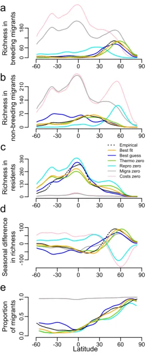
Figure 3: Latitudinal trends for empirical and simulated patterns in the global spatial distribution of terrestrial birds across seasons. Latitudinal trends were obtained using
Nadaraya–Watson kernel regression estimates (using the ksmooth function from the stats package in R), and were plotted for the empirical data (empirical, black dashed line), the overall best-fit model (best fit; orange line), the best-guess model (best guess, dark blue line), the best fit model without thermoregulation cost (thermo zero, green line), the best fit model without reproduction cost (repro zero, light blue line), the best fit model without migration
R ich ne ss in bre ed in g mi gra nt s -60 -30 0 30 60 90 0 60 180
a
R ich ne ss in no n-b re ed in g mi gra nt s -60 -30 0 30 60 90 0 70 140 210b
R ich ne ss in re si de nt s -60 -30 0 30 60 90 0 130 260 390 Empirical Best fit Best guess Thermo zero Repro zero Migra zero Costs zeroc
Se aso na l d iff ere nce in ri ch ne ss -60 -30 0 30 60 90 -1 00 0 100d
Pro po rt io n of mi gra nt s -60 -30 0 30 60 90 0.0 0.5 1.0e
Latitudecost (migra zero, grey line), and the best fit model without any energetic cost (no energy, pink line).
Figure 4: Predictive value of the overall best-fit model contrasted with the best-guess model and the null models. The best-guess model is based on parameters obtained from the
literature; no energy: null model that does not integrate energetic considerations (species selected randomly); costs zero: null model that does not account for energetic costs (distributions driven solely by energy supply); migra zero: best-fit model for the model without migration cost; thermo zero: best-fit model for the model without thermoregulation cost; repro zero: best-fit model for the model without reproduction cost. Predictive value
quantified as mean Earth Mover’s Distance values50 between simulated and empirical
patterns: the smaller the distance the better the match.
Earth Mover's Distance between empirical and simulated patterns
0 5000 10000 15000 No energy T he rmo ze ro R ep ro ze ro Mi gra ze ro Be st fi t Be st g ue ss C ost s ze ro
Energy efficiency drives the global seasonal distribution of birds
Supplementary Information
Marius Somveille1,2,3*, Ana S. L. Rodrigues3, Andrea Manica2
1Edward Grey Institute, Department of Zoology, University of Oxford, United Kingdom
2Department of Zoology, University of Cambridge, United Kingdom
3Centre d’Ecologie Fonctionnelle et Evolutive CEFE UMR 5175, CNRS - Université de
Montpellier - Université Paul-Valéry Montpellier – EPHE, France * [email protected]
SUPPLEMENTARY METHODS
Parameter fitting: best-fit model. We searched the four-dimensional parameter space of the
SEDS model for the combination of parameter values (α, β, γ, and µ) that best fit the empirical data. To quantify the similarity between a simulated and an empirical spatial pattern, we computed the Earth Mover’s Distance (EMD) between them. The EMD,
originally developed for image comparison1, provides a distance measure by calculating the
effort it takes to shape one pattern (defined on a discrete grid) into another (defined on the same discrete grid). The EMD is well adapted for our purpose of comparing simulated and empirical spatial patterns of species richness because (a) it quantifies how far apart (geographically) the two patterns are, and (b) it is sensitive to differences in the magnitude of species richness.
We used Pele & Werman’s fast algorithm for computing EMD1,2 implemented in Python
(FastEMD; https://github.com/wmayner/pyemd). FastEMD requires determining ground
distances between hexagons, with a threshold above which the cost associated with the distance in the EMD computation is maximal and constant. We used a threshold of 2000 km, which was a good compromise between computational limitations and visual pattern comparison. EMD values outputted by the FastEMD algorithm were standardised by dividing them by their corresponding sum of the flows. For each combination of parameter values, we compared the model outputs to the global empirical patterns by computing three EMD values: one for the richness in breeding migrants, one for the richness in non-breeding migrants, and one for the richness in residents. We then took the mean of these three values to obtain a single EMD value, used to quantify the fit of the model to the empirical data. To find the combination of parameter values that produced the simulated patterns that best match the observed ones (i.e. the ‘best-fit’ model), we used an optimization algorithm: the NSGAII
genetic algorithm via the OpenMOLE workflow engine (www.openmole.org). We used a
population size of 10 and stopped the algorithm when it appeared to have converged. We selected the combination of parameters producing the lowest EMD value from that last generation as our best-fit model.
Using this optimization algorithm, we explored the following extended parameter space: • 𝛼 ∈ 0, 0.0002 , 0 corresponding to no migration cost and 0.0002 corresponding to a
cost of migration of 20% of the yearly basal energy use for existence if the species travels an average of 1000 km between its breeding and non-breeding geographical ranges.
• 𝛽 ∈ 0, 80 , 0 corresponding to TLC = 40 and therefore a maximal cost of
thermoregulation everywhere across the world, and 80 corresponding to TLC = -40 and
therefore only a few places with extreme winter temperature where birds have a thermoregulation cost.
• 𝛾 ∈ 0, 2.25 , 0 corresponding to no reproduction cost and 2.25 corresponding to a cost of reproduction of 225% of the seasonal basal energy use for existence.
• 𝜇 ∈ 50, 110 , 50 corresponding to a low carrying capacity (1 unit of NDVI corresponded to 50 unit of energy supply) and 110 corresponding to a high carrying capacity (1 unit of NDVI corresponded to 110 unit of energy supply).
Supplementary Figure 1. Modelling the energetic costs of virtual species. Each species’
energetic costs were added on top of the basal energy use for existence (BEU, constant across
species and equals to 1 arbitrary unit of energy use) and comprised: migration cost (determined by parameter α), thermoregulation cost (determined by parameter β); and reproduction cost (during the breeding season; determined by parameter γ). dm: great circle
distance between the centroids of the breeding and non-breeding geographical ranges; TLC:
lower critical temperature of the thermoneutral zone; TA: ambient temperature. Body
temperature of birds assumed to be 40°C.
Parameter estimation: best-guess model. In order to investigate the biological realism of
each of the four parameter values obtained from the fitting procedure, we have compared these to coarse estimations obtained from the literature.
• Migration. The parameter α (which multiplied by distance travelled gives the migration cost; Fig. S1) can be estimated, based on flight physiology3, as equals to flight power (FW, in J/s) divided by flight speed (FS, in m/s). To rescale the cost of
migration in terms of the arbitrary units of energy use, we compared the energy used for the migratory journey to the basal metabolic rate (which approximates minimum levels of energy expenditure for existence) over a whole season (BMRS, in J), such
that: 𝛼 = !!
!! !"#!. Detailed comparative studies found that FW and FS scale with body
mass (M, in g) such that 𝐹! = 0.257𝑀!.!"# (estimated using data from Videler
(2007)4 on the cost of forward flapping flight for 31 avian species, excluding seabirds)
and 𝐹! = 6.4773𝑀!.!" (estimated by Alerstam et al. [2007]5 measuring the cruising speed of 138 species of migratory birds in flapping flight) respectively. We used the allometric relationship for the basal metabolic rate (BMR, in mlO2/h) described for
211 avian species by Fristoe et al. (2015)6 as: 𝐵𝑀𝑅 = 6.7141𝑀!.!"#$, which we then
converted to J/s using the conversion factor 1J/s = 172mlO2/h, and multiplied by the
number of seconds in 6 months (i.e. ~15,724,800) to obtain 𝐵𝑀𝑅! = 6.15𝑒!𝑀!.!"#$.
The resulting estimation for α was therefore approximately independent of body mass,
with the cost of migration equal to: 𝑚! = 6.45𝑒!!𝑑
!, with dm the travel distance in
kilometers. This corresponds to an energetic cost for migration of ~0.065 – or ~6.5% of the yearly basal energy use for existence if the species travels an average of 1000 km between its breeding and non-breeding geographical ranges.
• Thermoregulation. The parameter β is equal to thermal conductance C divided by the basal metabolic rate BMR, and indicates the lower limit of the thermo-neutral zone (Fig. S1). Both of these quantities have been shown to scale with body mass: Fristoe et
al. (2015)6, using data for 211 avian species, estimated that 𝐶 = 0.8248𝑀!.!"##, and
that 𝐵𝑀𝑅 = 6.7141𝑀!.!"#$, where M is the body mass (in g). The resulting
estimation for β was therefore 𝛽 = 8.1403𝑀!.!"#$ = 13.4 for an average bird of
38.6g. This corresponds to an energetic demand for thermoregulation of ~161% of the basal energy use for existence if a species experiences a mean temperature of 5°C across its seasonal geographical range.
• Reproduction. To estimate the parameter γ, we used data from Sibly et al. (2012)7 measuring the mass-specific reproductive output of 980 avian species as grams of eggs produced per grams of adult female per year. Re-analysing their data, we found a strong allometric relationship for the extra mass produced during the breeding season (not mass-specific; Me; Fig. S2) and estimated the corresponding extra energy cost as:
!"#!! !"# !!
! , where 𝐵𝑀𝑅!! = 6.7141(𝑀 + 𝑀!)!.!"#$ (ref
6). We divided by 2 because most bird species are monogamous and thus the extra mass is on average produced by two individuals. Fig. S2 shows the relationship between this extra energy cost and body mass. For an average bird of 38.6g, this corresponds to an estimated energetic cost for reproduction of γ=0.195, so 19.5% of the basal energy use for existence.
Supplementary Figure 2. Estimating the energy costs of reproduction. The extra mass (in g) produced through reproduction (= egg mass × number of eggs per clutch × clutch frequency), was obtained as log10(mass-specific productivity) + log10(body mass) (re-analysis of data on mass-specific
productivity and body mass in 7). The BMR of the extra mass was obtained by applying the BMR allometric equation to the sum of body mass and the extra mass produced and then dividing by BMR and subtracting 1.
We assume in the model that all species are equivalent in terms of their energetic requirements, not because we think this corresponds to reality, but in order to test how far a model can go without the need to integrate inter-specific variation in flight abilities, thermoregulation or reproduction strategies.
SUPPLEMENTARY RESULTS
Comparing parameters in best-fit and best-guess models. Deviations between best-fit
values for the full model and literature estimates (Fig. S8) are consistent with the type of empirical data on which the latter were based. First, the cost of migration was estimated as a simple linear function of the distance travelled. The slope estimated from previous studies on the cost of forward flapping flight3–5 was very similar to the one obtained from fitting the model to data. When thermoregulation cost was not included, the model performs very well and converges towards a cost of migration that is lower than the best-guess estimate, which is not necessarily unrealistic as birds commonly use flight strategies that results in energetic costs that are lower than direct flapping flight such as flying in V-formation8 and using
favorable weather conditions9. Second, the cost of thermoregulation was modelled as a linear
increase in energetic requirements outside of species’ thermo-neutral zone. The literature estimation for the lower limit temperature of the thermo-neutral zone, estimated from a
heat-transfer model10 and data from previous studies related to heat loss and thermal conductance6,
was higher than the one obtained from fitting the model (i.e. the model converged towards generally lower thermoregulation cost), which is not surprising as many bird species have
evolved cold-temperature adaptations such as seasonal molting11, changes in basal metabolic
rate6 and communal roosting12. Third, the cost of reproduction was modelled as the extra energy requirements during the breeding season for the production of new organisms. It was
over-predicted by the model, which is expected as birds, in addition to producing eggs, generally
expend energy on territorial defense, nest construction or incubation7.
Supplementary Figure 3. Contrast between empirical patterns in the global spatial distribution of terrestrial birds across seasons and the same patterns simulated through one of the simulations of the null model without energetic constraints (no energy model).
Latitudinal trends (black: empirical; red: simulated) were obtained using Nadaraya–Watson kernel regression estimates (using the ksmooth function from the stats package in R). In the scatterplots of the relationship between the empirical and simulated patterns, goodness-of-fit was computed using the sum of squared residuals from the 1:1 line (in red). In panel r, land hexagons with zero simulated species (for which the proportion of migrants could not be calculated) are coloured in grey.
Supplementary Figure 4. Contrast between empirical patterns in the global spatial distribution of terrestrial birds across seasons and the same patterns simulated through the null model without energetic costs (costs zero model). Latitudinal trends (black:
empirical; red: simulated) were obtained using Nadaraya–Watson kernel regression estimates (using the ksmooth function from the stats package in R). In the scatterplots of the relationship between the empirical and simulated patterns, goodness-of-fit was computed using the sum of squared residuals from the 1:1 line (in red). In panel r, land hexagons with zero simulated species (for which the proportion of migrants could not be calculated) are coloured in grey. Total number of virtual species simulated: 9188.
R2=-23.8 R2=-42.3 R2=-0.58 R2=-4.68 R2=-3.63 a e i qq r s t m j n o p k l f g h b c d
Supplementary Figure 5. Contrast between empirical patterns in the global spatial distribution of terrestrial birds across seasons and the same patterns simulated through the best-fit model without migration cost (migra zero null model). Latitudinal trends
(black: empirical; red: simulated) were obtained using Nadaraya–Watson kernel regression estimates (using the ksmooth function from the stats package in R). In the scatterplots of the relationship between the empirical and simulated patterns, goodness-of-fit was computed as the sum of squared residuals from the 1:1 line (in red). In panel r, land hexagons with zero simulated species (for which the proportion of migrants could not be calculated) are coloured in grey. Total number of virtual species simulated: 7545.
R2=-10.9 R2=-28.0 R2=-0.62 R2=0.52 R2=-3.42 a e i qq r s t m j n o p k l f g h b c d
Supplementary Figure 6. Contrast between empirical patterns in the global spatial distribution of terrestrial birds across seasons and the same patterns simulated through the best-fit model without reproduction cost (repro zero null model). Latitudinal trends
(black: empirical; red: simulated) were obtained using Nadaraya–Watson kernel regression estimates (using the ksmooth function from the stats package in R). In the scatterplots of the relationship between the empirical and simulated patterns, goodness-of-fit was computed using the sum of squared residuals from the 1:1 line (in red). In panel r, land hexagons with zero simulated species (for which the proportion of migrants could not be calculated) are coloured in grey. Total number of virtual species simulated: 10829.
R2=-1.09 R2=-4.41 R2=0.08 R2=-3.16 R2=0.41 a e i qq r s t m j n o p k l f g h b c d
Supplementary Figure 7. Contrast between empirical patterns in the global spatial distribution of terrestrial birds across seasons and the same patterns simulated through the best-fit model without thermoregulation cost (thermo zero null model). Latitudinal
trends (black: empirical; red: simulated) were obtained using Nadaraya–Watson kernel regression estimates (using the ksmooth function from the stats package in R). In the scatterplots of the relationship between the empirical and simulated patterns, goodness-of-fit was computed using the sum of squared residuals from the 1:1 line (in red). In panel r, land hexagons with zero simulated species (for which the proportion of migrants could not be calculated) are coloured in grey. Total number of virtual species simulated: 7829.
R2=0.64 R2=0.31 R2=0.42 R2=0.60 R2=0.64 a e i qq r s t m j n o p k l f g h b c d
Supplementary Figure 8. Parameter space explored by the optimisation algorithm, contrasting best-fit models and the best-guess model. Blue crosses: parameter values in the
best-guess model; orange crosses: parameter values in the full best-fit model; black crosses: parameter values in the best-fit models without one energetic cost (the one that is represented neither on the x-axis nor on the y-axis; e.g. the reproduction cost on the left-hand side plot).
α (migration cost) β (t he rmo re gu la tio n co st ) 0.00000 0.00005 0.00010 0.00015 0.00020 0 20 40 60 80 α (migration cost) γ (re pro du ct io n co st ) 0.00000 0.00005 0.00010 0.00015 0.00020 0.0 0.5 1.0 1.5 2.0 2.5 β (thermoregulation cost) γ (re pro du ct io n co st ) 0 20 40 60 80 0.0 0.5 1.0 1.5 2.0 2.5
Supplementary Figure 9. Contrast between empirical patterns in the global spatial distribution of terrestrial birds across seasons and the same patterns simulated through the best-guess model. Latitudinal trends (black: empirical; red: simulated) were obtained
using Nadaraya–Watson kernel regression estimates (using the ksmooth function from the
stats package in R). In the scatterplots of the relationship between the empirical and simulated
patterns, goodness-of-fit was computed using the sum of squared residuals from the 1:1 line (in red). In panel r, land hexagons with zero simulated species (for which the proportion of migrants could not be calculated) are coloured in grey. Total number of virtual species simulated: 7844. R2=0.53 R2=0.31 R2=0.49 R2=0.5 R2=0.44 a e i qq r s t m j n o p k l f g h b c d