Hybrid Energy-efficient Routing Protocol based on Cuckoo Search and Simulated Annealing algorithms

Ahmed Draia University - Adrar Faculty of Science and Technology

Department of Mathematics and Computer Science

A Thesis Presented to Fulfill the Master’s Degree in Computer Science Option: Intelligent Systems

Title

Hybrid Energy-efficient Routing Protocol based on

Cuckoo Search and Simulated Annealing algorithms

Prepared by

Siham FEROUHAT and Soulaf ZAKARIA

Supervised by

The problem of energy consumption in WSNs has become a very important axis of research. Hierarchical-based routing protocols have greatly contributed to the network scalability, lifetime and minimum energy consumption. In this work, we propose a novel hierarchical bio-inspired hybrid routing protocol based on cuckoo search (CS) algorithm and simulated annealing (SA) HRP-CSSA. Our proposed protocol takes the advantages of SA which avoid trapped in local minima, as well as properties of CS algorithm. The performance of the novel protocol is compared with the well known cluster-based protocol LEACH-C and ECSBCP protocol. Experimental results show that HRP-CSSA has the best performance in almost all metrics especially in terms of energy consumption.

Key words: WSNs, energy consumption, Simulated annealing, Cuckoo Search algorithm, CSSA, clustering, LEACH, ECSBCP

Résumé

Le problème de la consommation d'énergie dans les réseaux des capteurs sans fil est devenu un axe de recherche très important. Les protocoles de routage hiérarchiques ont grandement contribué à l'évolutivité du réseau, à sa durée de vie et à sa consommation d'énergie minimale. Dans ce travail, nous proposons un nouveau protocole de routage hybride bio-inspiré hiérarchique basé sur un algorithme de recherche de coucou (CS) et un recuit simulé (SA) HRP-CSSA. Notre protocole proposé prend les avantages de la SA, qui évitent de rester piégés dans les minima locaux, ainsi que les propriétés de l'algorithme CS. Les performances du nouveau protocole sont comparées aux protocoles bien connus LEACH-C et ECSBCP. Les résultats expérimentaux montrent que HRP-CSSA affiche les meilleures performances dans presque tous les indicateurs, notamment en termes de consommation d'énergie.

Mots clés: RCSFs, consommation d'énergie, recuit simulé, algorithme de recherche de coucou, CSSA, clusters, LEACH, ECSBCP

“Anything’s possible if you’ve got enough never” J.K.Rowling

My humble effort is dedicated to:

My Mother,

A strong and gentle soul who taught me to trust in Allah, believe in hard work

and that so much could be done with little, "May God have

mercy upon your soul"

To The dearest person,

My Father,

To My dear sisters Imane, who sacrificed herself for my happiness and my

success,

“may god bless you”.

To my little sister Wassila and my dear brothers Mohammed and Taha

Yacine, I wish a good continuation for their studies

I also dedicate this dissertation to my friends and all my family who have

supported me throughout this process. I will always appreciate all they have

done, especially: Khadidja, Mounia, Chahrazed, Sara, Soulaf, Karima, Marwa,

Siham, Khadidja and imane. I wish all the best for them

Every challenging work needs self efforts as well as guidance of elders

especially those who were very close to our heart.

My humble effort is dedicated to my sweet and loving

Father & Mother,

Whose affection, love, encouragement and prays of day and night make me able

to get such success and honor.

Along with all hard working and respected

Teachers

In the Name of Allah, the Most Merciful, the Most Compassionate, all praise be to Allah, the Lord of the worlds; and prayers and peace be upon Mohamed His servant and messenger.

First and Foremost praise is to ALLAH, the Almighty, the greatest of all, on whom ultimately we depend for sustenance and guidance. We would like to thank Almighty Allah for giving us opportunity, determination and strength to do our research. His continuous grace and mercy was with us throughout our life and ever more during the tenure of our research

We would like to express our deep and sincere gratitude to our supervisor Mr.Mohammed DEMRI. His wide knowledge and his logical way of thinking have been of great value for us. His invaluable comments, ideas, encouragement, and guidance have provided a good basis for the present thesis.

Our respect and gratitude to the jury members who gave us the honor of judging this work through their availability, observations and reports that have enabled us to enhance our scientific contribution.

We would like to thank Mr. BARMATI Mohammed for his help and guidance throughout this work.

Finally, our last thoughts are with our families, and especially our parents, for the sacrifices and the means they have put at our disposal to enable us to follow our studies in the best conditions.

Dedicates ... I Acknowledgements ... III Table of content ... IV Liste of figures ... VIII Liste of table ... X Liste of acronyms ... XI

General introduction ... 1

CHAPTRE I:GENERAL OVER VIEW OF WIRELESS SENSOR NETWORKS I.1. Background………..3

I.2. Sensor Node Architecture……….3

I.2.1. Definition………. 3

I.2.2 .Sensor Node Structure………. 3

I.1.2.1. Sensing Unit………4

I.1.2.2. Processing Unit.………..4

I.1.2.3. Power Unit………..4

I.1.2.4. Communication unit………4

I.1.2.5. The Memory/storage unit……….……...5

I.3. Wireless Sensor Network……….5

I.3.1. Definition……… 5

I.3.2. Characteristics of Wireless Sensor Networks……….5

I.3.2.1. Power efficiency……….5

I.3.2.2. Fault tolerance……….6

I.3.2.3. Mobility of nodes………6

I.3.2.4. Heterogeneity of nodes………...6

I.3.2.5. Scalability………6

I.3.2.6. Responsiveness………...…6

I.3.2.7. Communication failures………. 6

I.3.3.3 Deployment………..7

I.3.3.4 Fault Tolerance……….7

I.3.3.5 Design Constraints………7

I.3.3.6 Limited bandwidth………7

I.3.4. Protocol Stack of Wireless Sensor Networks………...8

I.3.4.1 physical layer………8

I.3.4.2 Data link layer………..8

I.3.4.3 Network layer………...9

I.3.4.4 Transport layer………..9

I.3.4.5 The application layer………9

I.3.4.6 The power management plane………..9

I.3.4.7 The mobility management plane………..9

I.3.4.8 The task management plane……….9

I.3.5. Application of Wireless Sensor Networks………..9

I.3.5.1. Military applications………...9

I.3.5.2. Area monitoring……….10

I.3.5.3. Structural monitoring……….10

I.3.5.4. Health applications………...11

I.3.5.5. Environmental applications………...12

1.6 Types of Wireless Sensor Networks ………..12

I.6.1 Terrestrial WSNs……… 13 I.6.2 Underwater WSNs………..13 I.6.3 Underground WSNs………14 I.6.4 Mobile WSNs………..14 I.6.5 Multimedia WSNs………...14 I.7. Conclusion………..15

II.1 Background………. . 16

II.2 Classification of Routing Protocols in WSN……… 16

II.2.1 Architecture Based Routing……….. 17

II.2.1.1 Data-Centric (DC) ………... 17

II.2.1.2 Hierarchical………...17

II.2.1.3 Location-based………..18

II.2.2 Operational Based Routing……… 18

II.2.2.1 Multipath Based Routing……… 18

II.2.2.2 Qos Based……… 18

II.2.2.3 Negotiation Based……… 19

II.2.2.4 Query Based……… 19

II.2.2.5 Non-coherent and Coherent Data-Processing Based………19

II.2.3 Route Selection………..19

II.2.3.1 Proactive Routing Protocols……….19

II.2.3.2 Reactive Routing Protocols………..20

II.2.3.3 Hybrid routing protocols………..20

II.3 Description of hierarchical routing protocols………20

II.3.1 Low Energy Adaptive Clustering Hierarchy (LEACH) ………..20

II.3.2 Low Energy Adaptive Clustering Hierarchy Centralized (LEACH-C) Protocol………..24

II.3.3 Power Efficient Gathering in Sensor Information Systems (PEGASIS) Protocol…………...25

II.3.4 Hybrid Energy Efficient Distributed Clustering (HEED) protocol………..27

II.4 Conclusion………29

CHAPTER III: OUR PROPOSED HYBRID ROUTING PROTOCOL III. 1. Background………30

III.2. Cuckoo Search: A Brief Literature Review……… 30

III.2.1 Biological foundations……….30

III.2.2. Cuckoo Search algorithm………31

III.2.3. Levy Flight………..32

III.3. Simulated annealing……….34

III.3.1 Annealing……… 34

III.3.2 Simulated Annealing………34

algorithms)……….…...37

III.4.1 Setup phase………..40

III.4.1.1 Cluster formation……….40

III.4.2 steady state phase……….42

III.5. The detailed flowchart of our proposed protocol………...42

III.6. Conclusion………...44

CHAPTER IV: SIMULATION, RESULTS AND DISCUSSION IV.1. Background………..45

IV.2. Developing environment: MATLAB……….. 45

IV.3. System model………...46

IV.3.1. Network model………46

IV.3.2. Energy dissipation model………46

IV.3.3. Hardware characteristics for MATLAB environment……… 47

IV.4. Description of Simulation interface……….48

IV.5. Simulation of the routing protocols……….50

IV.5.1 Number of rounds………51

IV.5.2 Residual energy………51

IV.5.3 Live Nodes………...53

IV.5.4 Control packets……….54

IV.5.5 Data delivery to BS………..55

IV.5.6 First dead node……….56

IV.6 discussion ………56

IV.7. Conclusion………...57

General Conclusion………... 58

Figure 1.1: Sensor Node ………3

Figure 1.2: Sensor Node Structure ……….4

Figure 1.3: Wireless Sensor Networks………5

Figure 1.4: Protocol Stack of Wireless Sensor Networks……….. 8

Figure 1.5: Military applications of WSN………..10

Figure 1.6: Area monitoring………10

Figure 1.7: Structural monitoring………11

Figure 1.8: Health applications………11

Figure 1.9: Environmental applications………..12

Figure 1.10: Terrestrial WSN………13

Figure 1.11: Underwater WSN……….13

Figure 1.12: Underground WSN……….. 14

Figure 1.13: Mobile WSN……….14

Figure 1.14: Multimedia WSN……….15

Figure 2.1: Classification of Routing Protocols in WSN………16

Figure 2.2: Flow chart of the Set-up phase of the LEACH protocol………..22

Figure 2.3: LEACH Protocol……….23

Figure 2.4: LEACH-C flow chart diagram……….24

Figure 2.5: Data transmission in PEGASIS……….26

Figure 3.1: Cuckoo………30

Figure 3.2: A cuckoo egg (green) in a host nest……….31

Figure 3.3: Cuckoo search algorithm………..33

Figure 3.4: Simulated annealing escaping from local optima……….. 36

Figure 3.5: Simulated annealing algorithm………..37

Figure 3.6: General flowchart of CSSA protocol………..39

Figure 3.7: Flowchart of cluster formation……….41

Figure 4.3: The Simulation result………. 49

Figure 4.4: The curves of simulation……….49

Figure 4.5: The lifetime of the network (CSSA, ECSBCP and LEACH-C)………51

Figure 4.6: Comparison of the residual energy versus No. of rounds………52

Figure 4.7: Comparison of the live nodes versus No. of rounds………53

Figure 4.8: Comparison of control packet versus No. of rounds……….. 54

Figure 4.9: Comparison of the data received by BS versus No. of rounds……… 55

Table 3.1: _{Classification of cuckoos}……… 31

Table 3.2: _{Analogy between the Physical System and the Optimization Problem}…. 35 Table 3.3: The profile of CSSA………. 38

Table 4.1: Hardware characteristics……….. 47

Table 4.2: Simulation parameters………. 50

Table 4.3: Simulation parameters of CS algorithm………. 50

Table 4.4: _{The residual energy versus each round for the} three protocols………….. 51

Table 4.5: _{Comparison of the live nodes versus No. of rounds for the three protocols} 53 Table 4.6: Control packets for each protocol……… 54

ACQUIRE: ACtive QUery forwarding In sensoR nEtworks ADC: Analog to Digital Converters

APTEEN: Adaptive Periodic TEEN BS: Base Station

CADR: Constrained Anisotropic Diffusion Routing CH: Cluster Head

CS: Cuckoo Search

CSMA: carrier–sense multiple access

HRP-CSSA: Hybrid routing protocol based on Cuckoo Search algorithm and Simulated Annealing

DC: Data-Centric

EAR: Energy Aware Routing

ECSBCP: Enhanced Cuckoo Search Based Clustering Protocol. GAF: Geographic Adaptive Fidelity

GBR: Gradient-Based Routing

GEAR: Geographic and Energy Aware Routing GPS: Global Positioning System

GUIs: Graphical User Interfaces

HEED: Hybrid Energy Efficient Distributed HPAR: Hierarchical Power-aware Routing

LEACH: Low Energy Adaptive Clustering Hierarchy LEACH-C: LEACH Centralized

MAC:Medium Access Control

MCFA: Minimum Cost Forwarding Algorithm MECN: Minimum Energy Communication Network

RAM: Random Access Memory SA: Simulated Annealing

SAR: Sequential Assignment Routing

SMECN: Small Minimum Energy Communication Network SNs: Sensor Nodes

SPEED: Stateless Protocol for Real-Time Communication in Sensor Networks SPIN: Sensor Protocol for Information via Negotiation

TDMA: Time Division Multiple Access

TEEN: Threshold sensitive Energy Efficient sensor Network TTDD: Two-Tier Data Dissemination

General Introduction

Advances in wireless communication and electronics has given rise to the creation of low-cost equipment, called sensor nodes or "motes", which can communicate via radio waves (radio) and collaborate with each other to form a wireless sensor network (WSN).

WSNs contain self-configured, distributed and autonomous Sensor Nodes (SNs) that monitor physical or environmental activities like humidity, temperature or sound in a specific area of deployment

The main problems in wireless sensor networks are the routing, the energy consumed by the nodes, the security, the data aggregation, the unpredictable mobility of the nodes, and so on. Sometimes deployed in hostile areas, so it is necessary to have an effective strategy that takes into account the energy of the network to increase its life span by reducing the loss of energy.

Researchers are heavily involved in designing energy efficient solutions; however, network lifetime can also be extended by planning energy efficient approaches. It is well accepted that cluster based hierarchical approach is an efficient way to save energy for distributed WSNs, which increase network life by effectively utilize the node energy and support dynamic WSNs environment. In a cluster based WSN, SNs are divided into several groups known as clusters with a group leader known as Cluster Head (CH). All the SNs sense data and send it to their corresponding CH, which finally send it to the BS for further processing. Clustering has various significant advantages over classical schemes. First, data aggregation is applied on data, received from various SNs within a cluster; to reduce the amount of data to be transmitted to BS thus energy requirements decrease sharply. Secondly, rotation of CHs helps to ensure balanced energy consumption within the network, which prevents getting specific nodes die due to lack of energy.

Our purpose is to introduce a new energy-efficient routing protocol to WSNs field that limits high energy consumption and enhance topology of the network through an efficient and reliable clustering mechanism.

In this thesis, we propose a hierarchical bio-inspired hybrid routing protocol based on cuckoo search (CS) algorithm and simulated annealing (SA) for WSNs namely HRP-CSSA for . This new protocol is based on hybrid between a bio-inspired algorithm that simulates the behavior of the cuckoo and the simulated annealing algorithm.

This thesis is organized as follow:

 Chapter one provides a general introduction to wireless sensor networks, presents its main characteristic, its challenges as well as its areas of application.

 The second chapter, presents a highlights the sections that cover classification of routing protocols in WSN and gives the principle overview of some protocols like LEACH, LEACH-C, PEGASIS and HEED.

 In the first part of Chapter three, we explain the principle of the cuckoo search and simulated annealing and in the second part, we present our proposed protocol.

 In the fourth Chapter, we gives an overview of MATLAB environment, the simulation results of our proposed protocols as well as comparison and analysis of different metrics such as throughput to the base station, number of rounds and residual energy.

 

 Finally, a conclusion is given to summarize our main contributions in addition to a section that describes our ideas of the future work.

CHAPTER I:

General overview of Wireless

Sensor Networks

I.1. Background

Wireless sensor networks are one of very important technologies today that is used for communications, so in this chapter, we discussed in details for general understanding of the concept of this study. First, highlights of Sensor Node Architecture and wireless sensor networks. Second, identify the biggest challenges of WSNs in addition to protocol stack. And finally, the applications areas of WSNs.

I.2. Sensor Node Architecture

I.2.1. Definition

A sensor node is a node in a wireless sensor network (WSN). This node is capable of sensing events, performing processing tasks on the detected events, and communicating the gathered data with other sensor nodes belonging to the same network [1].

Figure 1.1: Sensor Node

I.2.2 .Sensor Node Structure:

A sensor node made up of five basic components: The sensing unit, The processing unit , The communication unit , The power unit , The Memory/storage unit .

Figure 1.2: Sensor Node Structure [2] I.1.2.1. Sensing Unit

Usually consists of one or more sensors and analog- to – digital converters (ADCs). The sensors observe the physical phenomenon and generate analog signals based on the observed phenomenon. The ADCs convert the analog signals into digital signals, which are then fed to the processing unit [2].

I.1.2.2. Processing Unit

The processing unit usually consists of a microcontroller or microprocessor with memory which provides intelligent control to the sensor node [2].

I.1.2.3. Power Unit

The power unit is the power source of the sensor. Power is stored either in batteries or capacitors. Batteries, both rechargeable and non-rechargeable, are the main source of power supply for sensor nodes [2].

I.1.2.4. Communication unit

Consists of a short - range radio for performing data transmission and reception over a radio channel [2].

I.4.2.5. The Memory/storage unit

Storage in the form of random access and read-only memory includes both program memory (from which instructions are executed by the processor), and data memory (for storing raw and processed sensor measurements and other local information). The quantities of memory and storage on board a WSN device are often limited primarily by economic considerations, and are also likely to improve over time .[2]

I.3. Wireless Sensor Network

I.3.1. Definition

A wireless sensor network (WSN) is an infrastructure-less and self-organized network. It is composed of a group of sensor nodes, which communicate by electro-magnetic waves. Each sensor node acts as both a sensor and a wireless router. The fundamental functions of WSNs are sensing, data gathering, processing information on monitored objects and transferring the information to the base station [3].

Figure 1.3: Wireless Sensor Networks

I.3.2. Characteristics of Wireless Sensor Networks [4]

I.3.2.1. Power efficiency

Nodes are remotely located and don’t have direct power access. So, they have limited power capacity. Batteries are used as a power source.

I.3.2.2. Fault tolerance

Node is prone to failure. WSN is resilient, that is, it should have the ability to maintain network functionalities in case of node failures.

I.3.2.3. Mobility of nodes

Some nodes require mobility to increase communication efficiency or according to the type of applications.

I.3.2.4. Heterogeneity of nodes

Nodes in WSN are of different types but need to work cooperatively in a single network.

I.3.2.5. Scalability

In WSN nodes are densely deployed. So, WSN should be scalable to manage large number of nodes.

I.3.2.6. Responsiveness

WSN should be capable to adapt quickly to the changing topology through which sensor nodes are connected.

I.3.2.7. Communication failures

In WSN, it should be quickly informed to the base station or gateway node, when any node fails to exchange data with other nodes.

I.3.3. Challenges of Wireless Sensor Networks:

Wireless sensor networks have tremendous potential because they will expandability to monitor and interact remotely with the physical world. Sensors have the ability to collect vast amounts of unknown data. WSNs to become truly ubiquitous, a number of challenges and obstacles must be overcome

I.3.3.1 Energy

The sensor node lifetime typically exhibits a strong dependency on battery life. The constraint most often associated with sensor network design is that sensor nodes operate with limited energy budgets. The death of a node due to power failure can cause significant topological changes and may require re-routing of packets and reorganization of the network. Therefore, as most wireless sensors

are dependent on batteries, energy-saving forms of computation and communication are necessary [5].

I.3.3.2 Limited memory and storage Space

A sensor is a tiny device with only a small amount of memory and storage space for the code. In order to build an effective security mechanism, it is necessary to limit the code size of the security algorithm [5].

I.3.3.3 Deployment

Deployment means implementing the wireless sensor network in real world location. It is very laborious and cumbersome activity and depends on the demographic location of the application that how network will be deployed. At locations which are hard to reach, sensors are dropped from helicopter or may be in some locations sensors are placed according to some topology. A proper node deployment scheme can reduce the complexity of problems. Deploying and managing a high number of nodes in a relatively bounded environment requires special techniques [5].

I.3.3.4 Fault Tolerance

Sensor network should remain functional even if any node fails while the network is operational. Network should be able to adapt by changing its connectivity in case of any fault. In that case, well- efficient routing algorithm is applied to change the overall configuration of network [5].

I.3.3.5 Design Constraints

The primary goal of wireless sensor design is to create smaller, cheaper, and more efficient devices. A variety of additional challenges can affect the design of sensor nodes and wireless sensor networks. WSN have challenges on both software and hardware design models with restricted constraints [6].

I.3.3.6 Limited bandwidth

In wireless sensor nets, much less power is consumed in processing data than transmitting it. Presently, wireless communication is limited to a data rate in the

order of 10–100 Kbits/second. Bandwidth limitation directly affects message exchanges among sensors, and synchronization is impossible without message exchanges. Sensor networks often operate in a bandwidth and performance constrained multi-hop wireless communications medium [6].

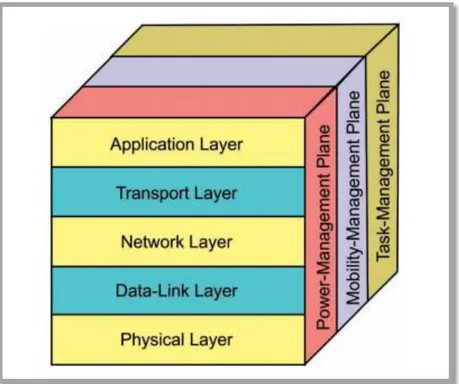
I.3.4. Protocol Stack of Wireless Sensor Networks:

The protocol stack used by sensor nodes to communicate with base station is shown in figure 2.9. According to Akyildiz [8], the protocol stack of WSN is almost like traditional network protocol stack with multiple layers: Application, Transport, Network, Data link, Physical layer, Power management plane, mobility management plane and task management plane. [9]

Figure 1.4: Protocol Stack of Wireless Sensor Networks

I.3.4.1 physical layer

The primary responsibilities of physical layer are frequency selection, carrier frequency generation, signal detection, modulation and data encryption [26].

I.3.4.2 Data link layer

Performs the tasks of data streams multiplexing, data frame detection, medium access and error control [26].

I.3.4.3 Network layer

is responsible for routing the information i.e. calculating the most efficient path of data transmission from source to destination. Network layer design in WSNs also considers energy efficiency, data-centric communication, data aggregation etc [26]. I.3.4.4 Transport layer

Performs the task of data flow maintenance especially when data captured by sensor nodes is to be accessed via internet or external communication networks [26] I.3.4.5 The application layer

Does the task of presenting all the information to specific application and forwarding requests from application layer to lower layers in protocol stack. The software in application layer depends on sensor application [26].

I.3.4.6 The power management plane

Is mainly responsible for minimizing power consumption in sensor nodes and waking up only those nodes required for packet transmission [26].

I.3.4.7 The mobility management plane

Detects and registers movement of nodes to maintain the route of sender node to sink node [26].

I.3.4.8 The task management plane:

Balances and schedules the sensing tasks to the sensing field and only specific nodes are assigned the sensing tasks and rest other nodes can perform other tasks like routing and data aggregation [26].

I.3.5. Application of Wireless Sensor Networks:

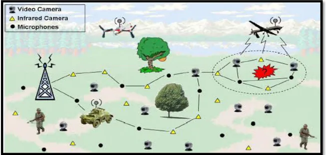
I.3.5.1. Military applications

Wireless sensor networks be likely an integral part of military command, control, communications, computing, intelligence, battlefield surveillance, reconnaissance and targeting systems [7].

Figure 1.5:Military applications of WSN

I.3.5.2. Area monitoring

In area monitoring, the sensor nodes are deployed over a region where some phenomenon is to be monitored. When the sensors detect the event being monitored (heat, pressure etc), the event is reported to one of the base stations, which then takes appropriate action.[7]

Figure 1.6: Area monitoring

I.3.5.3. Structural monitoring:

Wireless sensors can be utilized to monitor the movement within buildings and infrastructure such as bridges, flyovers, embankments, tunnels etc enabling

Engineering practices to monitor assets remotely without the need for costly site visits.[9]

Figure 1.7: Structural monitoring

I.3.5.4. Health applications:

Some of the health applications for sensor networks are supporting interfaces for the disabled, integrated patient monitoring, diagnostics, and drug administration in hospitals, tele-monitoring of human physiological data, and tracking & monitoring doctors or patients inside a hospital.[7]

I.3.5.5. Environmental applications

The term Environmental Sensor Networks has developed to cover many applications of WSNs to earth science research. This includes sensing volcanoes, oceans, glaciers, forests etc. There is some other major areas which are:

 Air pollution monitoring  Forest fires detection  Greenhouse monitoring  Landslide detection [7]

Figure 1.9: Environmental applications

1.6 Types of Wireless Sensor Networks

Depending on the monitoring environment, the sensor nodes forming sensor networks can be deployed underwater, underground, land or even space. The following are the five major types of WSN network:

a) Terrestrial WSNs b) Underwater WSNs c) Underground WSNs d) Mobile WSNs

I.6.1 Terrestrial WSNs:

In terrestrial WSNs, thousands of sensor nodes are deployed either in ad hoc manner or pre-planned manner and are efficient to communicate with base stations. Structured mode takes into consideration optimal placement, grid placement or 2D/3D placement models whereas in unstructured mode, the nodes are installed in random fashion over target area. Energy is the primary issue with terrestrial WSNs and energy retention can be done via low duty cycle operations, delay minimization and energy efficient routing protocols [27].

Figure 1.10: Terrestrial WSN

I.6.2 Underwater WSNs:

Underwater WSNs comprise of sensor nodes and sensor oriented vehicles to uniformly operate underwater. Autonomous underwater vehicles are deployed for capturing sensed data from sensor nodes. The chief issues surrounding underwater WSNs are long propagation delay, quality of service, energy and sensor failures due to underwater obstacles. [27]

I.6.3 Underground WSNs:

As compared to terrestrial WSNs, underground WSNs requires more cost in terms of deployment, maintenance and planning. Underground WSNs are deployed for monitoring underground conditions and communicate back to sink nodes above the ground. Sensor nodes are really difficult to charge and maintain, as nodes operate under the ground. Other issues surrounding underground WSNs are QoS wireless communications as signal loss and attenuation always occurs. [27]

Figure 1.12: Underground WSN

I.6.4 Mobile WSNs:

Mobile WSNs operate in physical environment for capturing real time data and are more versatile as compared to static sensor networks. Mobile WSNs are better in terms of area coverage, QoS, energy efficiency, better channel capacity etc. [27]

Figure 1.13: Mobile WSN I.6.5 Multimedia WSNs:

Multimedia WSNs perform the task of tracking and monitoring of events like imaging, audio, video etc. They are low cost sensor networks integrated with microphones and cameras and connect with other nodes in network via wireless communication for data compression, retrieval and correlation. [27]

Figure 1.14: Multimedia WSN

I.7. Conclusion

Wireless sensor networks are of considerable interest and a new step in the evolution of information and communication technologies. This new technology is attracting increasing interest given the diversity of these applications: healthcare, environment, industry and even in the security field.

We noticed that several constraints complicate the management of this type of network. Indeed, the sensor networks are characterized by a limited energy capacity that making the optimization of energy consumption in networks as a critical task to extend the life of the network.

In the next chapter, we make a study of the major Hierarchical routing protocol in these networks.

CHAPTER II:

Hierarchical Routing

Protocols in WSNs

II.1 Background:

Wireless sensor network is a network that consists of tiny, complex and large number of sensors and at least one base station or sink node. Most challenging issue in wireless sensor network is the limited battery power of sensor nodes used in the network. To increase the energy of sensor nodes, energy is preferably dispensed throughout the wireless sensor network. So the key to enhance the life time of the network is to design effective and energy aware protocols. Routing protocol can be network structure based or protocol operation based. In this chapter, a tutorial of existing routing protocols in wireless sensor networks is carried out.

II.2 Classification of Routing Protocols in WSN

Different routing protocols are proposed for WSN taking into account the challenges that affect the performance of routing protocols resulting in overall WSN performance degradation. These protocols can be classified according to different parameters as depicted with the classification tree in Figure 2.1.[10]

Figure 2.1: Classification of Routing Protocols in WSN

Routing Protocols for WSN Architecture Based Routing Data-Centric Hierarchical Location-based Operational Based Routing Multipath Based Routing QoS-Based Negotiation Based Query Based Coherent and Non-coherent Route Selection Proactive Reactive Hybrid

II.2.1 Architecture Based Routing

Protocols are divided according to the structure of network which is very crucial for the required operation. The protocols included in this category are further divided into three subcategories according to their functionalities.[10]

II.2.1.1 Data-Centric (DC)

In data-centric routing, the sink sends queries to certain regions and waits for data from the sensors located in the selected regions. Since data is being requested through queries, attribute-based naming is necessary to specify the properties of data [11]. The main idea of the DC is to combine the data coming from different sources en-route (in-network aggregation) by eliminating redundancy, minimizing the number of transmissions; thus saving network energy and prolonging its lifetime. Unlike traditional end-to-end routing, DC routing finds routes from multiple sources to a single destination that allows in-network consolidation of redundant data. [10]

Example: SPIN, Directed diffusion, Rumor Routing, GBR, CADR, ACQUIRE, MCFA, EAR and COUGAR

II.2.1.2 Hierarchical

The main aim of hierarchical routing is to efficiently maintain the energy consumption of sensor nodes by involving them in multi-hop communication within a particular cluster and by performing data aggregation and fusion in order to decrease the number of transmitted messages to the sink. Cluster formation is typically based on the energy reserve of sensors and sensor’s proximity to the cluster head [11]. Although this approach can provide higher network scalability, clustering operation and cluster head replacement (which is required to prevent fast energy depletion of the cluster heads) impose high signaling overhead to the network.[12]

Example: LEACH, TEEN, APTEEN, PEGASIS, HEED, LEACH-C and TTDD are hierarchical protocols because all nodes in network forward a message for a node that is in a higher hierarchy level than the sender.

II.2.1.3 Location-based

In this kind of network architecture, sensor nodes are scattered randomly in an area of interest and mostly known by the geographic position where they are deployed. They are located mostly by means of GPS. The distance between nodes is estimated by the signal strength received from those nodes and coordinates are calculated by exchanging information between neighboring nodes [12]. However, since localization support requires specific hardware components and imposes significant computational overhead to the sensor nodes, this approach cannot be easily used in resource-constrained wireless sensor networks.[10]

Examples: MECN, SMECN , GAF, GEAR, Geographic Routing in Lossy WSNs SAR, and SPEED

II.2.2 Operational Based Routing

WSNs applications are categorized according to their functionalities. Hence routing protocols are classified according to their operations to meet these functionalities. The rationale behind their classification is to achieve optimal performance and to save the scarce resources of the network. [12]

II.2.2.1 Multipath Based Routing

This type of routing protocols uses multiple paths instead of a single path in order to enhance network performance [13].

Example: Directed diffusion.

II.2.2.2 Qos Based

QoS based protocols are designed to satisfy QoS demands of different applications (e.g., delay, reliability, and bandwidth). The main aim of these approaches is to establish a trade-off between energy consumption and data quality. [10]

Example:In SAR, a sensor node selects a tree for data to be routed back to the sink according to energy resources and an additive QoS measure.

II.2.2.3 Negotiation Based

These protocols use high-level data descriptors in order to eliminate redundant data transmissions through negotiation. Communication decisions are also made based on the resources available to them [13].

Examples: SPIN family protocols.

II.2.2.4 Query Based

In this type of routing protocol destination nodes propagate a query for data (sensing task) from a node through the network, and a node with this data sends the data that matches the query back to the node that initiated the query [12]

Example: RUMOR, ACQUIRE, COUGAR

II.2.2.5 Non-coherent and Coherent Data-Processing Based

In non-coherent data processing routing, nodes will locally process the raw data before it is sent to other nodes for further processing. The nodes that perform further processing are called aggregators. Non-coherent functions have fairly low data traffic loading. In coherent routing, the data is forwarded to aggregators after minimum processing. The minimum processing typically includes tasks like time-stamping and duplicate suppression. To perform energy-efficient routing, coherent processing is normally selected. Since coherent processing generates long data streams, energy efficiency must be achieved by path optimality [13].

II.2.3 Route Selection

The WSN routing protocols can be further classified on the basis of path computation on the acquired information. This classification of protocol is based on how the source node finds a route to a destination node [10].

II.2.3.1 Proactive Routing Protocols

Are also known as table driven protocols which maintains consistent and accurate routing tables of all network nodes using periodic dissemination of routing information. In this category of routing all routes are computed before their needs [10].

GBR protocols classified into this category due to keep track of routes to all destinations in routing tables

II.2.3.2 Reactive Routing Protocols

These protocols are also called as On-Demand routing protocols as in these kind of routing protocols node searches for route on-demand i.e., whenever a node wants to send data it searches route for destination node and establishes the connection.[10]

II.2.3.3 Hybrid routing protocols

This strategy is applied to large networks. Hybrid routing strategies contain both proactive and reactive routing strategies. It uses clustering technique which makes the network stable and scalable. The network cloud is divided into many clusters and these clusters are maintained dynamically if a node is added or leave a particular cluster. This strategy uses proactive technique when routing is needed within clusters and reactive technique when routing is needed across the clusters. Hybrid routing exhibit network overhead required maintaining clusters [10].

Example: Rumor Routing, HPAR, GAF, and APTEEN protocols are an example of hybrid routing because their selection route based on a combination of proactive and reactive approaches

II.3 Description of hierarchical routing protocols

II.3.1 Low Energy Adaptive Clustering Hierarchy (LEACH):

This protocol is proposed by W. R. Heinzelman et.al which minimizes energy dissipation in sensor networks, It is based on a simple clustering Figure 2.3 mechanism by which energy can be conserved since cluster heads are selected for data transmission instead of other nodes. The operation of LEACH is broken up into rounds, where each round begins with a set-up phase, when the clusters are organized, followed by a steady-state phase, when data transfers to the base station

set-up phase. [16]

Set-up phase: During this phase, each node decides whether or not to become a cluster head (CH) for the current round. This decision is based on choosing a random number between 0 and 1. If number is less than threshold T(n), the node become a cluster head for the current round. The threshold value is set as:

if n

ϵ G

T(n)= (2.1)

Otherwise

Where:

P = desired percentage of cluster head, r = current round

G = the set of nodes which did not become cluster head in last 1

𝐏rounds.

Once the cluster head is chosen, it will use the CSMA MAC protocol to advertise its status. Remaining nodes will take the decision about their cluster head for current round based on the received signal strength of the advertisement message. Before steady-state phase starts, certain parameters are considered, such as the network topology and the relative costs of computation versus the communication. A Time Division Multiple Access (TDMA) schedule is applied to all the members of the cluster group to end messages to the CH, and then to the cluster head towards the base station. As soon as a cluster head is selected for a region, steady-state phase starts. Figure 2.2 shows the flowchart of this phase. [16]

𝑃

1 − 𝑃 ∗ (𝑟 ∗ 𝑚𝑜𝑑 1𝑝)

0

Figure 2.2 Flow chart of the Set-up phase of the LEACH protocol [14]

Steady-state phase: Once the clusters are created and the TDMA schedule is fixed, data transmission can begin. Assuming nodes always have data to send, they send it during their allocated transmission time to the cluster head. This transmission uses a minimal amount of energy (chosen based on the received strength of the cluster-head advertisement). The radio of each non-cluster-head node can be turned off until the nodes allocated transmission time, thus minimizing energy dissipation in these nodes. The cluster-head node must keep its receiver on to receive all the data from the nodes in the cluster. When all the data has been received, the cluster head node performs signal processing functions to generate the composite single signal. For example, if the data are audio or seismic signals, the cluster-head node can beam form the individual signals to generate a composite

away, this is a high-energy transmission. [14]

Advantages :

 LEACH is completely distributed. LEACH does not require the control information from the base station, and the nodes do not require knowledge of the global network in order for LEACH to operate. [15]

Disadvantages

 CH selection is random, that does not take into account energy consumption.

 It does not scale well to a large area.

 CHs are not uniformly distributed; CHs may be located at the edges of the cluster

Figure 2.3 LEACH Protocol

II.3.2 Low Energy Adaptive Clustering Hierarchy Centralized (LEACH-C) Protocol:

LEACH-C uses a centralized clustering algorithm and the same steady-state phase as LEACH. LEACH-C protocol can produce better performance by dispersing the cluster heads throughout the network. During the set-up phase of LEACH-C, each node sends information about its current location (possibly determined using GPS) and residual energy level to the sink. In addition to determining good clusters, the sink needs to ensure that the energy load is evenly distributed among all the nodes. To do this, sink computes the average node energy, and determines which nodes have energy below this average [14].

Once the cluster heads and associated clusters are found, the sink broadcasts a message that obtains the cluster head ID for each node. If a cluster head ID matches its own ID, the node is a cluster head; otherwise the node determines its TDMA slot for data transmission and goes sleep until it’s time to transmit data. The steady-state phase of LEACH-C is identical to that of the LEACH protocol [14].

The flowchart of LEACH-C algorithm is presented in Figure 2.4

Advantages:

 Since the base station has knowledge of the network and information of energy and location of sensor nodes, it forms better clusters that require less energy for transmitting data. A higher number of rounds is achieved in LEACH-C in small area networks.

Disadvantages :

 LEACH-C causes extra overhead on the BS. LEACH-C is not applicable for very large networks.

II.3.3 Power Efficient Gathering in Sensor Information Systems (PEGASIS) Protocol:

This protocol is proposed by Lindsey S., et al., is an improvement of LEACH. In PEGASIS only closing nodes communicate with each other and take turns being the leader for transmission to the sink. In PEGASIS, the position of nodes is random, and each sensor node has the ability of data detection, wireless communication, data fusion and positioning. Energy load is distributed evenly among the sensor nodes in the network. [16]

In PEGASIS, the nodes are arranged in order to form a chain, which can either be concentrated assigned by the sink and broadcast to all nodes or formed by the nodes themselves using a greedy algorithm. If the chain is formed by the nodes themselves, they can first get the location data of all nodes and locally compute the chain using the same greedy algorithm. During the process of chain formation in PEGASIS, it is assumed that all nodes have global knowledge of the network and the greedy algorithm is employed. The chain construction is started from the furthest node from the sink and the closest neighbor to this node will be the next node on the chain. When a node on the chain dies, the chain will be reconstructed in the same manner to bypass the dead node. [16]

For collecting data from sensor nodes in each round, each node receives data from its neighbor, fuses the data with its own, and transmits to the other neighbor on the chain. By moving from node to node, the fused data eventually are sent to the sink by the leader at a random position on the chain.The leader is important for nodes

places is to enhance the robustness of the network. Alternatively, in each round, a control token passing approach initiated by the leader is used to start the data transmission from the ends of the chain. The scheme of data transmission in PEGASIS is shown in Figure 2.5.

Figure 2.5 data transmission in PEGASIS

Advantages:

 This protocol is able to outperform LEACH for different network sizes and topologies, because it reduces the overhead of dynamic cluster formation in LEACH, and decreases the number of data transmission volume through the chain of data aggregation. [16]

 The energy load is dispersed uniformly in the network. To ensure that the fixed sensor node is not select as the leader and thus to prevent the subsequent early death of this sensor node, all sensor nodes act as the leader in turn. [16]

Disadvantages:

 It is the necessity of having a complete view of the network topology at each node for chain construction and that all nodes must be able to transmit directly to the sink. Thus, this scheme is unsuitable for those networks with a time varying topology [16];

 The communication manner suffers from excessive delays caused by the single chain for distant nodes and a high probability for any node to become a bottleneck. [16]

II.3.4 Hybrid Energy Efficient Distributed Clustering (HEED) protocol:

Introduced by Younis and Fahmy, is a multi-hop WSN clustering algorithm which brings an energy-efficient clustering routing with explicit consideration of energy. Different from LEACH in the manner of CH election, HEED does not select nodes as CHs randomly. The manner of cluster construction is performed based on the hybrid combination of two parameters. One parameter depends on the node's residual energy, and the other parameter is the intra-cluster communication cost. In HEED, elected CHs have relatively high average residual energy compared to MNs. Additionally, one of the main goals of HEED is to get an even-distributed CHs throughout the networks. Moreover, despite the phenomena that two nodes, within each other's communication range, become CHs together, but the probability of this phenomena is very small in HEED. [17]

In HEED, CHs are periodically elected based on two important parameters: residual energy and intra-cluster communication cost of the candidate nodes. Initially, in HEED, a percentage of CHs among all nodes, Cprob,

is set to assume that an optimal percentage cannot be computed a priori. The probability that a node becomes a CH is:

Where

E

E

maximum energy, which is typically identical for all nodes in the network. The value of

CH

selected to be inversely proportional to Emax. Afterwards, each node goes through

doubles its

CH

1. Therefore, there are two types of status that a sensor node could announce to its neighbors: tentative status and final status. If its CHprob is less than 1, the node

becomes a tentative CH and can change its status to a regular node at a later iteration if it finds a lower cost CH. If it's CHprobhas reached 1, the node

permanently becomes a CH. In HEED, every node elects the least communication cost CH in order to join it. On the other hand, CHs send the aggregated data to the BS in a multi-hop fashion rather than single-hop fashion of LEACH. [19]

Advantages:

 It is a fully distributed clustering method that benefits from the use of the two important parameters for CH election [17]

 Low power levels of clusters promote an increase in spatial reuse while high power levels of clusters are required for inter-cluster communication. This provides uniform CH distribution across the network and load balancing [17]

Limitations:

 The use of tentative CHs that do not become final CHs leave some uncovered nodes. As per HEED implementation, these nodes are forced to become a CH and these forced CHs may be in range of other CHs or may not have any member associated with them. As a result, more CHs are generated than the expected number and this also accounts for unbalanced energy consumption in the network [17]

 Some CHs, especially near the sink, may die earlier because these CHs have more work load, and the hot spot will come into being in the network

II.4 Conclusion

In this chapter we presented a thoroughly classification for routing protocols in WSNs. Many routing protocols, specially designed for sensor networks, are highly dependent on the network application. So, we have highlighted the characteristics of WSN's routing protocols from main five classification perspectives that we consider as most related to the network design. Among the design factors and challenges for WSN's protocols are the energy-awareness and scalability because of the numerous number of sensor nodes involved in the network design.

CHAPTER III:

Our proposed hybrid routing

protocol

III. 1. Background:

Historically bio-inspired algorithms have been extensively used in computational intelligence. Many researchers are working in this area and have developed different algorithms serving different purposes. One of the most interesting areas where these algorithms can be widely used is clustering in wireless sensor networks. In the literature, several bio-inspired optimization techniques have been investigated to solve NP-hard problems. In this chapter, we first preview in details the Cuckoo Search (CS) algorithm and the Simulated Annealing (SA) algorithm; then we present our proposed hybrid routing protocol based on CS and SA algorithms, namely HRP-CSSA.

III.2. Cuckoo Search: A Brief Literature Review

III.2.1 Biological foundations:

Cuckoos (scientific name: Cuculiformes) have three big families: Musophagidae, Cuculidae and Opisthocomidae. There are more than 100 species of cuckoos, but only one family of cuckoos lives in Europe, i.e., Cuculidae (Figure 3.1). Cuckoos are widespread in almost all areas in the world from Africa to Europe. They often feed on insects, especially caterpillars [38]

Figure 3.1: Cuckoo

In fact, the CS has been inspired by the brooding parasitism of some cuckoo species. This aggressive reproduction brooding parasitism acts as follows. A female cuckoo typicallylays 16 to 22 eggs that can be different in color and can match the eggs of the host.Different species may produce different colors, and they often target at different host birds. On the grey, yellow, green and red surface, eggs are often dotted with

21.9 to 16.3 mmin radius. Approximately half of cuckoo birds do not hatch their own eggs, but resort to such parasitism. A hidden female waits nearby the appropriate host nest for a chance of dumping its eggs in the host nest (Figure 3.2). Usually, newborn cuckoo chick can engage aggressive eviction of host birds’ eggs [39]. Biological classification of cuckoos is summarized in Table 3.1. [18]

Figure 3.2: a cuckoo egg (green) in a host nest.

Biological classification Kingdom Animalia Phylum Chordata Class Aves Order Cuculiformes Family Cuculidae

Table 3.1 Classification of cuckoos

III.2.2. Cuckoo Search algorithm:

CS is a swarm-intelligence-based algorithm that has been developed by Yang and Deb (2009), inspired by natural behavior of cuckoos, especially, the obligate brood parasitism’s of some cuckoo species by laying their eggs in the nests of other host birds. [18]

cuckoos in order to become appropriate for implementation as an computer algorithm:  Each cuckoo lays one egg at a time, and dumps it in a randomly chosen nest.  The best nests with high-quality eggs will be carried over to the next

generations.

 The number of available host nests is fixed and the egg laid by a cuckoo may be discovered by the host bird with a probability 𝑝_𝑎 ∈ (0, 1). In this case, the host bird can either get rid of the egg, or simply abandon the nest and build a completely new nest.

Regarding the mentioned rules, the CS was implemented as follows.

 Each egg in a nest represents a candidate solution. Thus, each cuckoo can lay only one egg into a nest in original form although each nest can has multiple eggs representing a set of solutions, in general. The task of CS is to generate the new and potentially better solutions that will replace the worse solutions in the current nest population. The quality of solutions is evaluated with the objective function of the problem to be solved. Normally, this function needs to be maximized.

 Mathematically, these kinds of problems are trivial to transform from minimization to maximization problems regarding equation min (f(x))=max(–

f(x)). In contrast objective function, such transformed function is now named as a fitness function.

 Furthermore, the last rule is approximated by an additional parameter 𝒑𝒂 named the switching probability that determine when the worst of the n host nests is replaced by a new randomly generated nest. In fact, this parameter balances two components of the CS process, i.e., exploration and exploitation as identified by Črepinšek et al. [41], where too much exploitation induces premature convergence, while too much exploration slows down the convergence.[18]

III.2.3. Levy Flight:

Levy flight is a random walk; the steps are defined regarding the step-lengths, which have a certain probability distribution, with the directions being random. This random walk can be observed in animals and insects. The next movement is based on the current position. [19].

Where α>0 is the step size. In most of the cases assume that α is equal to one. The product ⊕ means entry-wise multiplication i.e. Exclusive OR operation Levy flight is a random walk with random step size following a levy distribution

Levy~u=𝒕−𝛌 (1< λ ≤3) (3.2) This formulation leads to an advantage of CS algorithm compared to other metaheuristic method. The CS algorithm has more efficient randomization due to heavy-tailed of Lѐvy flights [19]

In the case of CS, the use of Levy Flight improves and optimizes the search: new solutions are generated by a random walk of Levy around the best solution obtained until now, which accelerates the global search.

Figure 3.3: cuckoo search algorithm [19]

III.3. Simulated annealing:

III.3.1 Annealing:

Annealing is the process of slowly cooling a heated metal in order to attain a minimum state of energy. This kind of idea to reproduce the annealing process has been efficiently exploited by Kirkpatrick et al. [42] to solve combinatorial optimization problems. The algorithm is initialized with a random solution to the problem being Begin

Objective function f(x), x = (x1, ...,xd)T ;

Initial a population of n host nests xi (i = 1, 2, ..., n); while (t <Max Generation) or (stop criterion)

Get a cuckoo (say i) randomly by Lévy flights; Evaluate its quality/fitness Fi;

Choose a nest among n (say j) randomly;

if (Fi >Fj)

Replace j by the new solution; End.

Abandon a fraction (pa) of worse nests and build new ones at new locations via Lévy flights; Keep the best solutions (or nests with quality solutions);

Rank the solutions and find the current best;

end while

Post process results and visualization;

coming down and by the side of every temperature.

In this case the number of attempts is made to agitate the present solution. At each agitated temperature, a change in the cost function ΔE is determined. If ΔE<0, then the proposed perturbation is accepted [43]

III.3.2 Simulated Annealing:

Simulated annealing applied to optimization problems emerges from the work of Kirkpatrick et al. [27] and V. Cerny [28]. In the 1980s, SA had a major impact on the field of heuristic search for its simplicity and efficiency in solving combinatorial optimization problems. Then, it has been extended to deal with continuous optimization problems [29, 30 and 31]. SA is based on the principles of statistical mechanics whereby the annealing process requires heating and then slowly cooling a substance to obtain a strong crystalline structure. The strength of the structure depends on the rate of cooling metals. If the initial temperature is not sufficiently high or a fast cooling is applied, imperfections (metastable states) are obtained. In this case, the cooling solid will not attain thermal equilibrium at each temperature. Strong crystals are grown from careful and slow cooling. The SA algorithm simulates the energy changes in a system subjected to a cooling process until it converges to an equilibrium state (steady frozen state). This scheme was developed in 1953 by Metropolis [32]. [24]

Table 3.2 illustrates the analogy between the physical system and the optimization problem. The objective function of the problem is analogous to the energy state of the system. A solution of the optimization problem corresponds to a system state. The decision variables associated with a solution of the problem are analogous to the molecular positions. The global optimum corresponds to the ground state of the system. Finding a local minimum implies that a metastable state has been reached. SA is a stochastic algorithm that enables under some conditions the degradation of a solution. The objective is to escape from local optima and so to delay the convergence. SA is a memory less algorithm in the sense that the algorithm does not use any information gathered during the search. From an initial solution, SA proceeds in several iterations. At each iteration, a random neighbor is generated. Moves that improve the cost function are always accepted. Otherwise, the neighbor is selected

degradation ∆E of the objective function. ∆E represents the difference in the objective value (energy) between the current solution and the generated neighboring solution. As the algorithm progresses, the probability that such moves are accepted decreases (Figure 3.5). This probability follows, in general, the Boltzmann distribution:

P (∆E, T) = exp (- (solution Energy – neighbor Energy)/ temperature) (3.3) It uses a control parameter, called temperature, to determine the probability of accepting no improving solutions. At a particular level of temperature, many trials are explored. Once an equilibrium state is reached, the temperature is gradually decreased according to a cooling schedule such that few non improving solutions are accepted at the end of the search. [24]

Table 3.2: Analogy between the Physical System and the Optimization Problem [24]

Physical System Optimization Problem

System states Solutions

Molecular positions Decision variables

Energy Objective function

Ground state Global optimal solution

Metastable state Local optimum

Rapid quenching Local search

Temperature Control parameter T

Figure 3.4: Simulated annealing escaping from local optima.

It can be clearly seen from the above figure that the higher the temperature, the more significant the probability of accepting a worst move. At a given temperature, the lower the increase of the objective function, the more significant the probability of accepting the move. A better move is always accepted. [24]

III.3.3 Algorithm Description:

a) Initial solution

The initial solution can be taken at random in the space of the possible solutions. This solution corresponds to an initial energy E = E0. This energy is calculated according to the criterion that one seeks to optimize. An initial temperature T = T0 high is also chosen.

b) Temperature Initialization

For better optimization, when initializing the temperature variable we should select a temperature that will initially allow for practically any move against the current solution.

c) Annealing schedule

The algorithm starts initially with T set to a high value (or infinity), and then it is decreased at each step following some annealing schedule that may be specified by the user, but must end with T = 0 towards the end of the allotted time budget. In this way, the system is expected to wander initially towards a broad region of the search space containing good solutions, ignoring small features of the energy function; then drift towards low-energy regions that become tight and tight; and finally move downhill . [48]