Power fluctuations in turbulence

O

pen

A

rchive

T

oulouse

A

rchive

O

uverte

(OATAO)

OATAO is an open access repository that collects the work of some Toulouse researchers and makes it freely available over the web where possible.

This is

an author's

version published in:

https://oatao.univ-toulouse.fr/23853

Official URL :

https://doi.org/10.1103/physrevlett.122.124504

To cite this version :

Any correspondence concerning this service should be sent to the repository administrator: tech-oatao@listes-diff.inp-toulouse.fr

Bos, Wouter J. T. and Zamansky, Rémi Power fluctuations in turbulence. (2019) Physical Review Letters, 122 (12). 1-6. ISSN 0031-9007

OATAO

Power fluctuations in turbulence

Wouter J. T. Bos1 and R´emi Zamansky2

1

LMFA, CNRS, Ecole Centrale de Lyon, Universit´e de Lyon, Ecully 69134, France

2_{Institut de M´ecanique des Fluides de Toulouse (IMFT), Universit´e de Toulouse, CNRS, Toulouse 31400, France}

To generate or maintain a turbulent flow, one needs to introduce kinetic energy. This energy injection

necessarily fluctuates and these power fluctuations act on all turbulent excited length scales. If the power is

injected using forces proportional to the velocity, such as those common in shear flows, or with a force

acting at the largest scales only, the spectrum of these fluctuations is shown to have a universal inertial

range, proportional to the energy spectrum.

DOI:10.1103/PhysRevLett.122.124504

During the famous 1961 conference on turbulence,

convincing evidence was presented in support of

Kolmogorov’s 1941 theory [1] of turbulence. Indeed a

measurement of the energy spectrum EðkÞ in a tidal channel

[2] showed a power law scaling proportional to k−5=3.

At the same conference, Kolmogorov himself presented a correction to his theory[3]. Inspired by a remark of Landau, he illustrated that the 1941 picture of an inertial range depending on the mean energy flux was flawed, since large spatiotemporal fluctuations of the energy flux, determined by the energy injection mechanism, should lead to a

correction of the −5=3 power law scaling. It was realized

that scaling relations could depend on the, necessarily nonuniversal, energy injection mechanism.

However, the energy injection might be more universal than perhaps expected. The reason for this is that the energy input is not only determined by the precise input mecha-nism, but also by the impedance of the flow itself. Clearly, a force cannot work if it is applied orthogonal to the velocity of a fluid element. The work done by a force through its interaction with a flow is investigated in the present Letter. The fluctuations of the energy input, or power, have been studied previously, in particular in experimental flows

between rotating disks [4,5]. Some universality was

observed in the shape of the probability density functions

(PDFs)[6,7]. A model for the shape of these PDFs could be

derived using a Gaussian assumption [8]. Further

inves-tigations of the power fluctuations include a numerical study of shear flow[9]and an investigation of the particular

case of wave turbulence [10]. More recently the study

of power fluctuations was revisited in the context of

Lagrangian statistics [11,12]. The related quantity of

subgrid-flux fluctuations, important for large eddy simu-lation strategies, was considered in some detail[13,14].

Most of these studies investigated the PDF of the power fluctuations, not their spectrum. Only minor attention was

given to temporal spectra in experiments [15]. In wind

farms, the spectral distribution of the power spectrum has

received some more attention, since electricity fluctuations are directly related to the power fluctuations in the

incoming turbulence [16–20]. These studies exclusively

focus on the time domain.

We will focus here on the wave number spectrum of the power fluctuations in turbulence using theoretical consid-erations and direct numerical simulations (DNSs). It will be shown that the power fluctuation spectrum contains a universal scaling range at high Reynolds numbers even when the probability density function of the fluctuations can differ from flow to flow.

We consider the incompressible Navier-Stokes equa-tions, and in particular the fluctuations of the velocity ui¼ Ui− hUii, where Uiðx; tÞ is the velocity field and

the angular brackets denote an ensemble average. In a statistically homogeneous flow the fluctuations are governed by

∂tuiþ ∂jðuiujÞ ¼ −∂ip þ νΔuiþ fi ð1Þ

combined with the constraint ∂_iui¼ 0. The fluctuating

pressure is indicated by p, ν is the kinematic viscosity and f is the applied force field per unit mass of fluid. The kinetic energy balance takes a particularly simple form

dthKi ¼ hPi − hϵi; ð2Þ

where the energy is given by K ¼ uiui=2 and ϵ is the

dissipation and the energy injection is given by,

P ¼ uifi: ð3Þ

Obviously in a steady state we havehPi ¼ hϵi, But locally

there is no reason for P ¼ ϵ. We can define the fluctuations by P0¼ P − hPi and ϵ0¼ ϵ − hϵi, and it is in particular P0 that we will focus on.

Let us start by answering the following question: is it possible to define a forcing such that P0is zero everywhere?

In other words, is it possible to inject the same amount of energy uniformly in space? Since it is only possible to inject energy if the scalar product of the velocity and the applied force is nonzero [see Eq. (3)], it is impossible to inject energy in stagnation points of the flow. Furthermore,

since ui is a continuous, zero-mean quantity, stagnation

points will exist and, at these points, no energy can be injected. Therefore, even if we control perfectly the applied force, in practice no turbulent flow can exist without power fluctuations. Power fluctuations are thus ubiquitous and we will investigate some of their properties in the following.

We will in the following consider the forcing

fi¼ αijujþ βi; ð4Þ

whereα_ijandβ_iare both functions of space and time, and whereβ is the component of the force orthogonal to the local velocityu. It is thus the part that does not inject energy. This forcing is fairly general. For instance, in a large class of turbulent flows the energy of the fluctuating turbulent field is supplied by the average velocity field, which corresponds to the case α_ij¼ ∂_jhU_ii. The linear forcing scheme, widely used in DNS[21]corresponds toα_ij¼ αδ_ij.

We will consider the specific case where α is not

determined by the fluctuating flow properties, but only by externally imposed parameters. The case of homo-geneous shear flow is an academic example of such a forcing. The average injected energy is then given by

hPi ¼ αijhuiuji ð5Þ

and evidently β does not appear in this expression. The

variance of the fluctuations is given by hP02_{i ¼ α}

ijαmnhuiujumuni − hPi2: ð6Þ

Working out a Gaussian estimate for the fourth order velocity correlations, we find

IP≡

hP02_i

hPi2 ¼

αijαmnðhuiumihujuni þ huiunihujumiÞ

hPi2 : ð7Þ

For the linear forcing we find then, using isotropy,

IP¼ 2=3, whereas for homogeneous shear ∂zhUxi we have

IP¼ 1 þ ρ−2uw; ð8Þ

with ρ_uw ¼ huwi=ðhu2i1=2hw2i1=2Þ, where u and w are velocity fluctuations in the streamwise and cross-stream direction, respectively. We have therefore the interesting feature that the energy injection intensity is directly related to the anisotropy of the flow. In experiments and

simu-lations of homogeneous shear flow [22]ρ_uw¼ Oð0.5Þ so

that IPis around 5. The Gaussian estimate shows therefore

that the injection intensity can strongly vary between

different flow types. What we will now investigate is how these fluctuations vary as a function of scale.

The fluctuation spectrum is defined as EPðkÞ ¼

Z

jkj¼khP

0_ðkÞP0_ð−kÞidS

k ð9Þ

where the integration is performed over spherical shells of radius k (the wave number) such that

Z

EPðkÞdk ¼ hP02i: ð10Þ

In these and following expressions, Fourier coefficient are

recognized by their argument (k, p, or q). The power

spectrum writes then EPðkÞ ¼

Z

jkj¼k

ZZ

hfiðpÞuiðk − pÞfjðqÞujð−k − qÞi

× dpdqdSk: ð11Þ

Without further information on the nature of the forcing

functionf, we cannot make any predictions on the scaling

of the spectrum EPðkÞ. We will therefore consider the

following two specific cases. The first one is a compact forcing at the large scales. The second one is a forcing reminiscent of the influence of a mean velocity gradient on a turbulent flow.

In the first case, where the forcing is confined to the largest scales, or smallest wave numbers, we can follow a reasoning similar to the one of Batchelor, Howells, and Townsend in deriving the shape of the temperature

spec-trum in low Prandtl number convection [23]. Let us

consider thatf acts at the smallest wave numbers around

jkj ¼ kf, while we are interested in the scaling of EPðkÞ for

k ≫ kf. In this range of scales (jk − pj ≫ jpj) we can

assume statistical independence of the velocity mode fiðpÞ

and uiðk − pÞ, so that we can split the fourth order

correlation, EPðkÞ ≈

Z

jkj¼k

ZZ

hfiðpÞfjðqÞihuiðk − pÞujð−k − qÞi

× dpdqdSk: ð12Þ

Furthermore, orthogonality of Fourier coefficients, and k − p ≈ k leads to,

EPðkÞ ≈ hfifjiϕijðkÞ ð13Þ

whereϕ_ijðkÞ¼R_jkj¼khu_iðkÞu_jð−kÞidS_kandϕ_iiðkÞ¼2EðkÞ. We see that when the forcing is constrained to the large scales, the power-spectrum is proportional to the spectral tensorϕ_ijðkÞ. In the case of an isotropic forcing, this shows that

EPðkÞ ≈

2

3hfifiiEðkÞ: ð14Þ

This result shows that, for an isotropic large-scale forcing, the power spectrum scales proportional to the energy spectrum. The fluctuations of the energy injection remain thus not confined to the forced scales but are distributed over all scales.

We can now ask what the relevance of this result is in the case where the forcing is not an artificial forcing confined

around kf, but where the kinetic energy is generated

through the interaction of the turbulence with an externally imposed velocity gradient. In that case we cannot directly assume independence of the forcing spectrum and the velocity modes at large wave numbers in order to simplify

Eq. (11). Let us consider the simplest case, fi¼ αui,

corresponding to a linear forcing, acting on all scales. Since we have in this case a direct relation between the power and the kinetic energy, P ¼ fiui¼ 2αK, the power spectrum is

now,

EPðkÞ ¼ 4α2EKðkÞ; ð15Þ

where EKðkÞ is the kinetic energy fluctuation spectrum

such that, Z

EKðkÞdk ¼ hðK − hKiÞ2i: ð16Þ

Since the integral of this spectrum yields the square of the kinetic energy fluctuations, a fourth order velocity corre-lation, one might expect that it does not scale like the kinetic energy spectrum, which is associated with a second order velocity correlation. This is actually not so, and the asymptotic wave number dependence of both spectra is the

same. Indeed, the spectrum EKðkÞ has received some

attention in the past [24–27], and is known to scale as

EKðkÞ ∼ huiuiiEðkÞ: ð17Þ

Therefore, even in this case where the forcing is not constrained to the largest scales, the small scales are

obeying a sweeping scaling [28]. Such results are fairly

robust, even when flows are not strictly isotropic. Indeed, the first evidence of the validity of Gaussian (or sweeping) scaling for higher-order spectra was obtained in mixing

layer and atmospheric boundary layer flows[24]. We will

check these ideas now.

We carried out direct numerical simulations (DNS) of isotropic turbulence in a periodic box at a resolution of 5123_{grid points. Details of the pseudospectral code can be}

found in Refs. [29,30]. Three different types of forcing

were considered. f1: a deterministic forcing keeping the

volume-averaged energy at the large scales constant [31].

This forcing was applied at the wave modes with k < 2pffiffiffi2.

f2.: a stochastic forcing where the energy injection is given

by an Ornstein-Uhlenbeck process[32], also applied at the

wave modes with k < 2pffiffiffi2. f3: a linear forcing, fi¼ αui

[21,33] applied to all scales. These forcing procedures

allow the turbulence to reach a statistically steady state with

a Reynolds number Rλ≈ 130 along with η=Δx ≈ 0.75,

withη ¼ ν3=4=ϵ1=4.

In our simulations a close to statistically steady state is obtained where the mean production equals approximately the mean dissipation. The normalized variance of the

dissipation rate fluctuations hϵ02i=hϵi2≈ 1.6 for the

three flows. The values of the variance of the power

fluctu-ations are however significantly different, hP02i=hϵi2¼

1.1; 4.2; 0.8 (for f1; f2; f3, respectively). This difference is

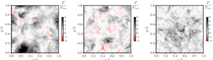
also illustrated in the visualizations of the power during the steady state, shown in Fig.1. It is observed that the power fields are qualitatively different. For instance, in the third forcing scheme the injected power can only be positive, whereas negative values are observed in the other two cases.

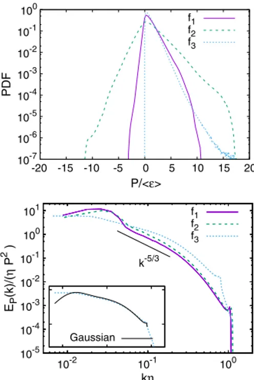
This is further illustrated in Fig. 2(a), where it is

observed that the PDFs of the power are very different in shape. On the contrary, the PDFs of the dissipation rate fluctuations are nearly identical (not shown). Analytical expressions can be derived for the power fluctuation PDFs assuming Gaussianity of the velocity fluctuations, at least for forcing f3, where the shape of the PDF should resemble

aχ2distribution. We will not further focus on this, but we stress that the shapes of the PDFs indicate that the power fluctuations generated by the three different forcing schemes are quite different.

In Fig.2(b)it is shown that the length scale distribution is not so different. The spectra of forcing scheme 1 and 2 are

very similar, with a power law exponent close to−5=3. The

third forcing yields a power fluctuation spectrum that is

shallower, with a slope close to−1. It seems thus that for

the first two forcing schemes, which are confined to the largest scales, the predicted scaling is observed. However, for the linear forcing, applied at all scales, a strong deviation is observed. In the following we will try to understand this difference. In particular we will show that also for this case a−5=3 scaling is expected to appear, be it at higher Reynolds numbers.

The statistical independence, invoked to derive the scaling relations is in the present case equivalent to the

FIG. 1. Visualizations of the power input in the turbulent flows.

From left to right forcing schemes f1, f2, and f3.

~

~

L:

~I O

.:

4

~

R

~

~

~I

,:.:

O 4

~

·

,

~

~

~

~I J J ~. J 0.2 . 0.2 -1-11 _ _ ...,__--1 0.0 0.0 0.2 0.4 0.6 0.8 1.0 0.0 0.2 0.4 0.6 0.8 1.0 0.0 0.2 0.4 0.6 0.8 1.0 ~ ~ ~

assumption of Gaussianity. Indeed, the sweeping scaling was derived by assuming joint-Gaussian velocity statistics

[24,27]. Even though Gaussian estimates give for certain

quantities good order-of-magnitude estimates, certain features are completely missed. For instance, the net energy transfer between scales is zero for joint-Gaussian velocity fluctuations. Furthermore, the dissipation rate fluctuations are severely mispredicted if Gaussianity is

assumed[34–36]. Is this the case here?

The Gaussian estimate of the power spectrum for linearly forced isotropic turbulence is

EPðkÞ ¼ 2kα2 Z Δð1 − x 2_{ÞEðpÞEðqÞ}dp p dq q ; ð18Þ

where x ¼ ðp · qÞ=pq and Δ indicates a subdomain in the p, q plane where the wave vectors k, p, q can form a triangle. This integral can be evaluated numerically for a given energy spectrum. We have, to check the assumption of Gaussianity, compared the power spectrum from the DNS

with the Gaussian prediction, using in Eq.(18)the energy

spectrum computed from the DNS data. The comparison is

shown in the inset of Fig. 2(b). The Gaussian prediction,

computed from the DNS energy spectrum, very accurately collapses with the actual power spectrum, except for the smallest wave numbers. This different behavior is due to the different nature of the boundary conditions in the two approaches. Indeed, the theoretical, integral Gaussian

estimate [Eq. (18)] assumes an infinite domain and

periodicity is not taken into account. Nevertheless, for all wave numbers in the inertial and dissipation range, the agreement is very good.

The actual reason that the power spectrum for the linear forcing is not proportional to k−5=3is that universal scaling appears at higher Reynolds numbers. In order to illustrate this, we carried out closure simulations of the eddy damped quasi normal Markovian type. Indeed the convergence to asymptotic statistics, as compared to experiments or sim-ulations, is well predicted by this closure scheme[37]. We have computed, using the linear forcing, steady states at

Reynolds numbers ranging from 100 to104. We used the

energy spectra from these simulations to compute the Gaussian estimate of the power spectrum. The results

are shown in Fig. 3. It is shown that a good collapse is

possible if the spectra are normalized by the mixed scaling [Eq.(14)], involvinghu_iuii; ϵ, and η. Indeed, in Fig.3we

plot ˜ EP¼ EPðkηÞ α2_hu iuiiϵ2=3η5=3 ; ð19Þ

and the good collapse of these normalized spectra shows the validity of Eq.(14). Furthermore it is observed that for the closure results, the convergence of the spectrum to asymptotic scaling is very slow. In the inset of Fig.3it is

observed that at Rλ¼ 100 the power law exponent is close

to −1, as for the DNS, but that the spectrum becomes

gradually steeper, attaining close to asymptotic scaling

around Rλ¼ 104. DNS at higher resolution and Reynolds

number should be able to assess this tendency to some extent, since the largest simulations of isotropic turbulence

[38]allow currently to reach Reynolds numbers of the order

of Rλ≈ 2 × 103.

With respect to the general applicability of the present insights one could object that the linear forcing fi¼ αuiis

rather artificial, but the ideas can be transposed to shear flow. Indeed, shear is the principal turbulent kinetic energy injection mechanism in the absence of body forces. In the

10-7 10-6 10-5 10-4 10-3 10-2 10-1 100 -20 -15 -10 -5 0 5 10 15 20 PDF P/<ε> f₁ f2 f₃ 10-5 10-4 10-3 10-2 10-1 100 101 10-2 10-1 100 k-5/3 EP (k)/( η P 2 ) kη f1 f₂ f₃ Gaussian

FIG. 2. (a) DNS results for the PDFs of the power fluctuations

for three different forcing schemes. (b) Power fluctuation spectra for the same three cases. In the inset we compare the spectrum for

forcing f3with its Gaussian estimate.

10-4 10-2 100 102 104 106 108 10-5 10-4 10-3 10-2 10-1 100 k-5/3 E ~ P (k η ) kη 102 103 104 1 1.2 1.4 1.6 1.8 102 103 104 n_u nP 1 1.2 1.4 1.6 1.8 102 103 104 n_u nP

FIG. 3. Gaussian estimates for EpðkÞ, computed from spectral

closure results using Eq. (18). Inset: spectral index nu of the

inertial range scaling of the energy spectrum and nP,

correspond-ing to the power law exponent of the power fluctuation spectrum

as a function of the Reynolds number Rλ.

-- -I ' - - - - - -1 '.' , \.,'',, ... . ', ' ... '

~

==

\. ',, ', _·. ' ' ··.. \ ·• _\ ' _' ·. _., ' _'

~

'\~:

case of steady uniform shear S ≡ ∂zhUxi, the energy input

is P ¼ −Shuwi. The power spectrum for this case is EPðkÞ ¼ S2EuwðkÞ, where the shear-stress fluctuation

spec-trum defined as Z

EuwðkÞdk ¼ hðuwÞ2i − huwi2: ð20Þ

It was shown[39,40]that also this spectrum is proportional to the trace of the spectral tensor and thereby scales as k−5=3, so that the above arguments for isotropic turbulence can be transposed to the very important case of shear flow. We showed that for a turbulent flow displaying the Kolmogorov energy spectrum, the power spectrum will reflect this scaling, following Eq.(14). Thereby the input fluctuations have a universal equilibrium range. Of course, it is possible to define a forcing function that will lead to different scaling, for instance, a forcing spectrum with a peak at the large wave numbers. However, as long as the support of the forcing function is confined to large wave

numbers, or with a power-law spectrum steeper than k−1,

the power spectrum will be given by Eq.(14). The next step in understanding turbulence intermittency is now the investigation of the fluctuations of the energy flux and its relation to the power fluctuations in order to understand if universality is also conserved for that quantity. The answer to that question definitely needs further research.

This work was performed using HPC resources from GENCI-CINES.

[1] A. N. Kolmogorov, The local structure of turbulence in incompressible viscous fluid for very large Reynolds

num-bers, Dokl. Akad. Nauk SSSR30, 301 (1941).

[2] H. L. Grant, R. W. Stewart, and A. Moilliet, Turbulence

spectra from a tidal channel,J. Fluid Mech.12, 241 (1962).

[3] A. N. Kolmogorov, A refinement of previous hypotheses concerning the local structure of turbulence in a viscous

incompressible fluid at high Reynolds number, J. Fluid

Mech.13, 82 (1962).

[4] R. Labb´e, J.-F. Pinton, and S. Fauve, Power fluctuations in

turbulent swirling flows,J. Phys. II6, 1099 (1996).

[5] O. Cadot, Y. Couder, A. Daerr, S. Douady, and A. Tsinober, Energy injection in closed turbulent flows: Stirring through

boundary layers versus inertial stirring,Phys. Rev. E56, 427

(1997).

[6] S. T. Bramwell, P. C. W. Holdsworth, and J.-F. Pinton, Universality of rare fluctuations in turbulence and critical

phenomena,Nature (London)396, 552 (1998).

[7] J.-F. Pinton, P. C. W. Holdsworth, and R. Labb´e, Power

fluctuations in a closed turbulent shear flow,Phys. Rev. E

60, R2452 (1999).

[8] M. M. Bandi, S. G. Chumakov, and C. Connaughton, Probability distribution of power fluctuations in turbulence,

Phys. Rev. E79, 016309 (2009).

[9] J. Schumacher and B. Eckhardt, Fluctuations of energy

injection rate in a shear flow,Physica (Amsterdam)187D,

370 (2004).

[10] E. Falcon, S. Aumaître, C. Falcón, C. Laroche, and S. Fauve, Fluctuations of Energy Flux in Wave Turbulence,

Phys. Rev. Lett.100, 064503 (2008).

[11] H. Xu, A. Pumir, G. Falkovich, E. Bodenschatz, M. Shats,

H. Xia, N. Francois, and G. Boffetta, Flight–crash events in

turbulence,Proc. Natl. Acad. Sci. U.S.A.111, 7558 (2014).

[12] A. Pumir, H. Xu, G. Boffetta, G. Falkovich, and E. Bodenschatz, Redistribution of Kinetic Energy in Turbulent

Flows,Phys. Rev. X4, 041006 (2014).

[13] S. Cerutti and C. Meneveau, Intermittency and relative scaling of subgrid-scale energy dissipation in isotropic

turbulence,Phys. Fluids10, 928 (1998).

[14] T. Aoyama, T. Ishihara, Y. Kaneda, M. Yokokawa, K. Itakura, and A. Uno, Statistics of energy transfer in high-resolution direct numerical simulation of turbulence in a

periodic box,J. Phys. Soc. Jpn. 74, 3202 (2005).

[15] J. H. Titon and O. Cadot, The statistics of power injected in a closed turbulent flow: Constant torque forcing versus

constant velocity forcing,Phys. Fluids15, 625 (2003).

[16] P. Milan, M. Wächter, and J. Peinke, Turbulent Character of

Wind Energy, Phys. Rev. Lett.110, 138701 (2013).

[17] R. Calif and F. G. Schmitt, Multiscaling and joint multi-scaling description of the atmospheric wind speed and the

aggregate power output from a wind farm, Nonlinear

Processes Geophys.21, 379 (2014).

[18] K. Viestenz and R. B. Cal, Streamwise evolution of

stat-istical events in a model wind-turbine array,

Boundary-Layer Meteorol.158, 209 (2016).

[19] M. M. Bandi, Spectrum of Wind Power Fluctuations,Phys.

Rev. Lett.118, 028301 (2017).

[20] J. Bossuyt, C. Meneveau, and J. Meyers, Wind farm power fluctuations and spatial sampling of turbulent boundary

layers,J. Fluid Mech.823, 329 (2017).

[21] T. Lundgren, Linearly forced isotropic turbulence, Annual Research Briefs 461 (2003).

[22] S. B. Pope, Turbulent Flows (Cambridge University Press, Cambridge, 2000).

[23] G. K. Batchelor, I. D. Howells, and A. A. Townsend, Small-scale variation of convected quantities like temperature in

turbulent fluid. Part 2,J. Fluid Mech.5, 134 (1959).

[24] C. W. Van Atta and J. C. Wyngaard, On higher-order spectra

of turbulence,J. Fluid Mech.72, 673 (1975).

[25] M. Nelkin and M. Tabor, Time correlations and random

sweeping in isotropic turbulence, Phys. Fluids A 2, 81

(1990).

[26] T. Ishihara, Y. Kaneda, M. Yokokawa, K. Itakura, and A. Uno, Spectra of energy dissipation, enstrophy and pressure by high-resolution direct numerical simulations

of turbulence in a periodic box,J. Phys. Soc. Jpn.72, 983

(2003).

[27] W. J. T. Bos and R. Rubinstein, On the strength of the

nonlinearity in isotropic turbulence,J. Fluid Mech.733, 158

(2013).

[28] H. Tennekes, Eulerian and Lagrangian time microscales in

[29] R. Zamansky, F. Coletti, M. Massot, and A. Mani, Turbulent

thermal convection driven by heated inertial particles, J.

Fluid Mech.809, 390 (2016).

[30] M. Gorokhovski and R. Zamansky, Modeling the effects of small turbulent scales on the drag force for particles below

and above the Kolmogorov scale, Phys. Rev. Fluids 3,

034602 (2018).

[31] S. Chen, G. D. Doolen, R. H. Kraichnan, and Z.-S. She, On statistical correlations between velocity increments and locally averaged dissipation in homogeneous turbulence,

Phys. Fluids A5, 458 (1993).

[32] V. Eswaran and S. B. Pope, An examination of forcing in

direct numerical simulations of turbulence,Comput. Fluids

16, 257 (1988).

[33] C. Rosales and C. Meneveau, Linear forcing in numerical simulations of isotropic turbulence: Physical space

imple-mentations and convergence properties, Phys. Fluids 17,

095106 (2005).

[34] H. Chen, J. R. Herring, R. M. Kerr, and R. H. Kraichnan,

Non-Gaussian statistics in isotropic turbulence,Phys. Fluids

A1, 1844 (1989).

[35] T. Gotoh and R. S. Rogallo, Intermittency and scaling of

pressure at small scales in forced isotropic turbulence, J.

Fluid Mech.396, 257 (1999).

[36] W. J. T. Bos, R. Chahine, and A. V. Pushkarev, On the scaling of temperature fluctuations induced by frictional

heating,Phys. Fluids27, 095105 (2015).

[37] W. J. T. Bos, H. Touil, and J.-P. Bertoglio, Reynolds number dependency of the scalar flux spectrum in isotropic

turbu-lence with a uniform scalar gradient, Phys. Fluids 17,

125108 (2005).

[38] T. Ishihara, K. Morishita, M. Yokokawa, A. Uno, and Y. Kaneda, Energy spectrum in high-resolution direct

numeri-cal simulations of turbulence,Phys. Rev. Fluids1, 082403

(2016).

[39] W. K. George, P. D. Beuther, and R. E. A. Arndt, Pressure

spectra in turbulent free shear flows,J. Fluid Mech.148, 155

(1984).

[40] C. Tong, Spectra of scalar-flux and stress fluctuations in

the atmospheric surface layer, J. atmos. Sci. 54, 1277