Control and design of multi-use induction machines : traction, generation, and power conversion

(1)

Control and Design of Multi-Use Induction Machines:

Traction, Generation, and Power Conversion

by

Al-Thaddeus Avestruz

S.B.

in Physics, Massachusetts Institute of Technology (1994)

Submitted to the Department of Electrical Engineering and Computer Science

in partial fulfillment of the requirements for the degree of

Master of Science

at the

MASSACHUSETTS INSTITUTE OF TECHNOLOGY

May 2006

@

Massh1.. ne++c Tr +if-iitp nf Tpnc',h-1nlnv

§T006. All rights reserved.

BARKER

Author ...

Departmentef'Electrical Englneering and Computer Science

25 May 2006

Certified

Steven B. Leeb

Professor of Electrical Engineering and Computer Science

Thesis Supervisor

Accepted by ...

Hrtnur C. Smit

Chairman, Department Committee on Graduate Students

MASSACHUSEMS INSTITUTE OF TECHNOLOGY

NOV 0 22006

LIBRARIES

(2)

(3)

Control and Design of Multi-Use Induction Machines: Traction, Generation,

and Power Conversion

by

Al-Thaddeus Avestruz

Submitted to the Department of Electrical Engineering and Computer Science on 25 May 2006, in partial fulfillment of the

requirements for the degree of Master of Science

Abstract

An electrical machine can be made to convert electrical power while performing in its primary role of transforming electrical energy into mechanical energy. One way of doing this is to design the machine with multiple stator windings where one winding acts as a primary for drive and power, and the others as secondaries for electrical power. The challenge is to control the mechanical outputs of torque and speed while independently regulating the electrical outputs of voltage and current. This thesis analyzes and demonstrates an approach that takes advantage of topological symmetries in multiphase systems to overcome this challenge. This method is

applied, but not relegated to induction machines.

Thesis Supervisor: Steven B. Leeb

(4)

(5)

Acknowledgments

I would like to thank my advisor Professor Steven Leeb for his efforts, patience, encouragement, and confidence in me, without which, all of this would not be possible.

To Meelee Kim, for her unwavering love and support.

To my parents, Suzanne and Fred, and my grandparents for their prayers and love: Lola Beth, Lola Jeannette, and Lolo Nes, who started my interest in science and engineering. In loving memory of my grandfather Alfonso Palencia.

To my brother Mark, without whose many discussions, I would have a lesser perspective of my work. To my sister Camille, whose future I look forward to with great confidence.

To Robert Cox, Chris Laughman, and Warit Witchakool for the many technical discus-sions that made work so much more interesting. To my office-mate Brandon Pierquet, for the discussions and entertainment and for the solutions to the little annoyances in LaTex.

And to everyone else in LEES, especially Professors Kirtley and Perreault, and to Vivian Mizuno.

I am sure to have forgotten to mention many who have helped me, but I am grateful despite the short lapse in memory.

This work was supported by the Center for Materials Science and Engineering, a Materials Research Science and Engineering Center funded by the National Science Foundation under award number DMR 02-13282, and by the Grainger Foundation.

(6)

(7)

Approximations of Sine Function 87 . . . 87 . . . 97 . . . 97 . . . 98 . . . 98 . . . 98 . . . 98 . . . 98 . . . 99 101 101 105 C Field Oriented Control Simulink Model C.1 Block Models . . . . C.2 Induction Motor S-Function . . . . D Motor Control Embedded Firmware D.1 Main Motor Control Module . . . . D .1.1 m ot-cntl.c . . . . D.1.2 umacros.h . . . . D.2 Sine Inverter PWM Module . . . . D.2.1 sin-pwm.c . . . . D.2.2 Header Files . . . . D.2.3 sin-pwm.h . . . . D.3 Volts per Hertz Module . . . . D.3.1 vfcontrol.c . . . . 113 . . . 113 . . . 113 . . . 123 . . . 126 . . . 126 . . . 132 . . . 133 . . . 135 . . . 135 63 65 66 69 69 70 71 71 71 75 77

(9)

Table of Contents

D.3.2 vfcontrol.h . . . 142

D.4 Serial Communications M odule . . . 143

D.4.1 serialcomm .c _{. . . 143}

D.4.2 serialcomm .h . . . 150

D.5 Peripheral Driver M odule . . . 151

D.5.1 periphs.c . . . 151

(10)

(11)

List of Figures

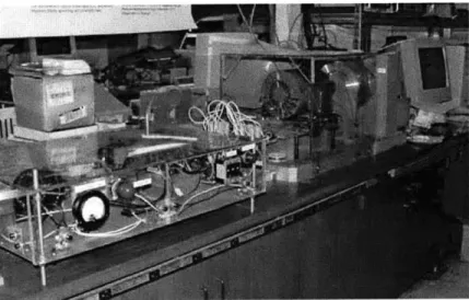
1.1 _{Photograph of Multi-Use Induction Motor Testbed . . . 18}

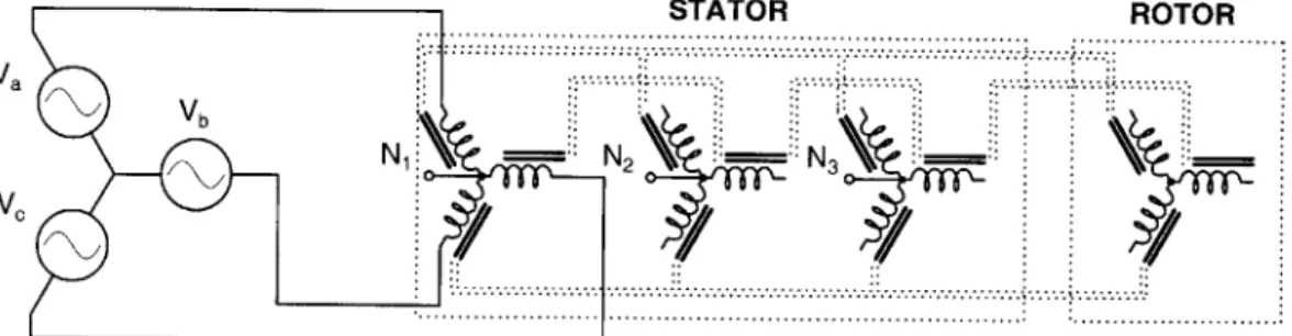
1.2 _{Multi-Stator Induction Machine . . . 19}

2.1 _{Electrical Model of Three-Legged Transformer . . . 24}

2.2 _{Transformer Model In-Circuit for Identical Stators Wound In-Hand . . . 25}

2.3 Effect of Series Inductance in the 3rd Harmonic Control Function . . . 26

2.4 Multiple Stator Connections Driving Three-Phase Rectifiers. . . . 27

2.5 _{Drive Waveform with Third Harmonic . . . 28}

2.6 _{3d Control Surface for Peak Amplitude Control . . . 29}

2.7 _{Third Harmonic Peak Amplitude Control Plotted Parametrically with Phase . . 30}

2.8 PI Control of Dc Output Using ₃rd Harmonic . . . 31

2.9 _{T-Model for the Zero Sequence Circuit. . . . 32}

2.10 Zero sequence transformer. _{. . . 33}

2.11 Direct zero sequence transformer. . . . 34

2.12 Exogenously driven zero sequence transformer. . . . 34

2.13 Utilization and Scaling Using Triple Insulated Wire . . . 37

3.1 DQ-Space Contour and Allowed Trajectory in Synchronous Current Regulator Saturation . . . 44

3.2 Simulation of induction motor under field-oriented control with speed and torque load steps. . . . 46

3.3 Implementation of a Field-Oriented Speed Controller for a Multi-Use Induction M achine . . . 48

4.1 _{International Rectifier's Integrated Power Module . . . 50}

4.2 _{Sine Reference from 108-element DLT . . . 52}

4.3 _{THD and Maximum Error versus Table Length for Direct Lookup Table . . . 52}

4.4 _{Inverter Voltage Waveforms . . . 53}

4.5 _{Inverter Current for Fundamental + 25% Third Harmonic . . . 53}

4.6 _{Error from Half-Wave Parabolic Sine Approximations . . . 57}

4.7 Errors from Quarter-Wave Parabolic Approximations to a Sine . . . 59

4.8 _{Line-to-line Three Phase Filter . . . 61}

(12)

s-4.9 Phase-to-Neutral Three Phase Filter . . . . 62

4.10 Coupled Inductor Three Phase Filter . . . . 64

4.11 Recovery of Rotor-Linked Current from Linear Combination of Stator Current M easurem ents . . . . 66

4.12 FFT of Stator Currents in Rotor-Linked Current Recovery . . . 67

5.1 Activity Diagram for Closed-Loop Control of Dc Output . . . 72

5.2 Activity Diagram for Synchronous Current Controller . . . 73

A.1 PSPICE Schematic-Wye-Ungrounded . . . 78

A.2 PSPICE Schematic-Wye-Grounded . . . 81

A.3 PSPICE Schematic-Wye-Grounded with Zero Sequence Transformer . . . . 84

C.1 Top Level M odel . . . 102

C .2 Speed Controller . . . 103

C.3 Field Oriented Controller . . . 104

C.4 Induction Motor Model . . . 105

(13)

(14)

(15)

List of Tables

3.1 Aardvark Machine Parameters _{. . . 45}

4.1 THD and Maximum For a DLT Sine Reference Using Different Interpolating Functions . . . 51

4.2 _{Coefficients for Half-Wave Sine Approximations . . . 58}

4.3 _{Coefficients for Quarter-Wave Sine Approximations . . . 60}

5.1 _{Examples of Task Timing . . . 70}

(16)

(17)

Chapter 1 Introduction

Jjicierncy, economy arid elegance are

hallmarks

of good design. The idea of

multi-use machines is an attempt to mitigate the waste and superfluity that is needlessly epidemic in a contemporary world starved of energy.

Motor and generator drives have been and continue to be crucial to a wide range of industrial and commercial products and manufacturing processes; among these, variable speed drives (VSDs) that operate over a range of mechanical shaft speeds are invaluable. Since the beginning, folks have found ways to vary the shaft speed of a motor; many exist, but circuit design and components in power electronics have advanced to a point were it is more appealing, both in performance and economics, for motors to be combined with power electronics in commercial and industrial VSDs.[1]

Many products use VSDs, including modern air handling and ventilation systems that run fans at speeds and power that are optimal, ensuring occupant comfort while keeping energy consumption to a minimum. Other examples include computer-controlled machine tools such as mill machines and lathes that need continuously variable speeds for different materials and tasks; hybrid and electric vehicles (EVs) use variable speed drives for traction or propulsion. These systems typically use power electronics to control the flow of power to the motor in controlling the speed. In addition to needing power for their drives, these systems often include other power supplies that typically includes distribution through a network of power buses through different parts of the system.

(18)

Figure 1.1: Photograph of what we have fondly called the Aardvark machine.

1.1 Machines with Multi-Use Capability

An electrical machine can be made to convert electrical power while performing in its primary role of transforming electrical energy into mechanical energy. One way of doing this is to design the machine with multiple stator windings where one winding acts as a primary for drive and power, and the others as secondaries for electrical power. The challenge is to control the mechanical outputs of torque and speed while independently regulating the electrical outputs of voltage and current.

The salient feature in these multi-use machines is the integration of magnetics for traction, generation and power conversion. While it is not eminently clear whether there is a convincing scaling law advantage in size and weight with this type of integration, it is evident that there is an economy to using the same control and power electronics for multiple purposes. Beyond rudimentary calculations for simple integrated pole face geometries, detailed studies of scaling laws for a variety of structures and magnetic circuit configurations is largely outside the scope of this work and is an obvious topic for follow-on research in machine design.

This thesis report analyzes and demonstrates an approach that takes advantage of topo-logical symmetries in multi-phase systems to overcome this challenge. This method has been applied, but not relegated to induction machines.

(19)

Section 1.2 : Design Challenges and Innovations

STATOR ROTOR

Va

Vb=

N ==N ===N ==

Figure 1.2: Simplified Depiction of a Multi-Stator Induction Machine.

1.2 Design Challenges and Innovations

There are a number of design challenges that must be addressed before one can assert whether this technology is viable for commercial and industrial applications. Overcoming the first challenge of proof of concept in a previous thesis [2] opened an avenue for continued research.

The first of the questions asks how one provides a wide range and monotonic control of the dc secondary output. It is answered by the use of the 3rd harmonic amplitude at a phase of 7r

radians for closed-loop control of the output; in general, the control-to-output function for dc output voltage is non-monotonic for other values of phase. Also, a look in [2] shows that the control of dc output using zero sequence phase, while effective, only provides a narrow range of variation.

The next addresses an issue that is endemic in most contraptions that we would like to use for multi-use machines: it is that of vanishingly small zero sequence reactance. A good solution, while not universal, is a variety of topologies that use a zero sequence transformer to improve the magnetizing inductance in the zero sequence circuit. Another solution, of course, is to redesign the machines, but that is the topic for another thesis.

Then, we must talk about the inverter. Not only must it be very good sinusoidal current source, but it must also be a very good voltage source of 3rd or other zero sequence harmonics;

it is the way you integrate the idea of zero sequence voltage with a field-oriented controller that is based on stator currents, which is the established means for variable speed drive.

This begs the question of generality. We talk for example about cars having two independent dc buses for power: the new one is 42 volts and the legacy is 12V. We can perhaps increase the number of phases in the machine so that there is more than one set of "independent" zero sequence harmonics. There are a number of ways to handle this: one can have a machine that physically has a greater number of inherent phases; the other, is to create these additional phases with linear combinations of the inherent phases. So, we start take a look at general

(20)

n-phase circuits that provide supernumerary zero sequence harmonic sets, and heterophasic transformer circuits.

How far can we go? As always, it depends on the compromises that one is willing to accept. It also matters how well we can design the machine, and this depends on at least an initial understanding of the design limitations and scaling laws. The complement to "how far" is "where else" and this is a question about machines other than induction ones. A glance at the ubiquity of the Lundell alternator adds not only to the intellectual, but also to the economic

appeal.

This work provides some of the foundations and proof-of-concepts.

1.3 Previous Work

Initial work and construction of the induction machine testbed had been performed by Jack W. Holloway in a previous thesis project [2]. This work included the demonstration of dc output control of a wye-grounded winding by varying the phase of the added 3rd harmonic in the

inverter and the independence to zero sequence harmonics of an identical winding with the wye ungrounded.

(21)

Chapter 2 Power Conversion Control By Zero

Sequence Harmonics

Zero sequence current in a multi-phase system is the portion of current that runs in the same direction through all the connection phases at the same time. This means that this component of the current has the same amplitude and angular phase in every connection phase.1 It is the part that we can consider "common-mode" to all phase connections: the vector sum of the currents in these phases.2

One can also speak of a zero sequence voltage. If the circuit has a balanced terminal

impedance and a zero sequence path, then it is that portion of the voltage at each phase that creates a zero sequence current. Often, we describe a zero sequence voltage in a way that is similar to a zero sequence current: having the same amplitude and angular phase in every connection, but it is not necessarily the case that a zero sequence voltage results in zero sequence current, as it is also the case that a positive or negative sequence voltage can result in a zero sequence current.

2.1 Induction Machine Model

A three phase induction machine can be described by the magnetic flux linkages among three

stationary windings (stator) and three moving windings (rotor). Equation 2.1a describes every permutation of how the flux through every winding is linked to a current in its own and every

'To avoid ambiguity, we make a distinction in this paragraph between connection phase, which is the actual physical connection to the circuit, and angular phase, which is the constant parameter in the argument of a periodic function that for the moment we assume to be unmodulated.

2

Though a Fourier transform, periodic signals can be represented as a sum of sinusoids. These sinusoids in turn can be represented as phasors.

(22)

others' winding. [3]

[

S __ [Ls LSR] iS

1

AR] LSR LR iR

where the stator flux in the stationary reference frame

the rotor flux

Aas

\s = Abs

Aar

-\R= Abr

.Acr.

and the mutual inductance matrix between the stator and the rotor

Lc cos 0r LSR Lc cos(Or - 27r/3) Le cos(Or + 27r/3) Lc cos(Or + 27r/3) Lc cos 0, Lc cos(Or - 27r/3) L, cos(Or - 27r/3)1 L, cos(Or + 27r/3) L, cos Or _{_}

When one applies the well-known Park's transform

[4]

cos 0 - sin 0 1 27r cos _(0~ 3 - sin 0- 1 1

and for completeness delineating its inverse

cos 0 COS ( -Io 6+ 27r 3 27r 3/ (2. 1a)

L[

= _Lab Lab Lr - Lab .Lab Lab Ls Lab Lab Lr Lab (2.1b) Lab

Fas

Lab _ibs L8 _

LiS,

Lab tar Lab tbr Lr _ icrJ (2.1c) (2. 1d) T = 2 3 cos

(0

- sin ( 27r 1+ 2-(2.2a) - sin 0 -sin

(o--sin (0+

11

1. 27r 3) 27r 3) (2.2b) ~s.. 22 n T-1 _

(23)

Section 2.1 : Induction Machine Model

to 2.1a, the flux linkages become block matrices, each of which are diagonal and time-invariant,

Adqs Ls M

[iq(

A~iqI

]'

I(2.3a)

[~

Adgr M LR idqr where [Las

ol

LS = , (2.3b) 0 Las (2.3c) LR = Lar 0 (2.3d) 0 Lar] (2.3e) M = 0 (2.3f) 10 M (2.3g) 3 M = 3Lc. (2.3h) 2

The state equations for the induction motor using flux are given by

-Ads = rsids - wAqs - Vds (2.4a)

-Aqs = rsiqs + WAds - Vqs (2.4b)

-Adr = rridr - wsAqr (2.4c)

-Aqr = rriqr + wsAdr, (2.4d)

and torque of electrical origin by

Tm = 3P(Aqridr - Adrzqr), (2.5)

and the equations of motion by

where(Tm - ti) , _(2.6)

where p is the number of pole pairs, J is the moment of inertia, and TI is the load torque.

(24)

2.2 A Transformer Model for a Stator with Multiple

Windings

Each phase in the stator windings is shifted by 120 electrical degrees; e.g. the flux linked between phase a and phase b is given by

Lab = L, cos(1200) = Lc.

2 (2.7)

Usually, the coupling is symmetric as well as equal among the phases, i.e., Lab = Lac = Lba =

In a machine with multiple stators, additional flux linkages exist between the stator wind-ings. Between two stators,

As,] [Ls1 M12 is:] (2.8)

As2] M21 Ls is2

In the next section, one will see how this bears more than just a casual similarity to a three-legged, three-phase transformer. In fact, the multiple stators of an induction by themselves behave the same way as the transformer illustrated in Figure 2.1, despite being wrapped around a circle. ia ib ic --- 1 Lc/2 Lc/2 - -- - - - - - -* - - -Lc/2 Lc/2 2 -) --- --- 1 I Lc/2 Lc/2 (a) kp kp kp (b)

Figure 2.1: Electrical model for the primary of a Three-Legged Transformer. kp is the phase-to-phase coupling coefficient.

The coupling coefficient between windings of a transformer is the fraction of the flux coupled

(25)

Section 2.2 : A Transformer Model for a Stator with Multiple Windings

between the primary and the secondary and is given by

kz M

L₁L₂ (2.9a)

which generalizes to a matrix element

kman Mmn

LmLn (2.9b)

that relates an arbitrary winding to another, where L1 and L2 are the primary and secondary

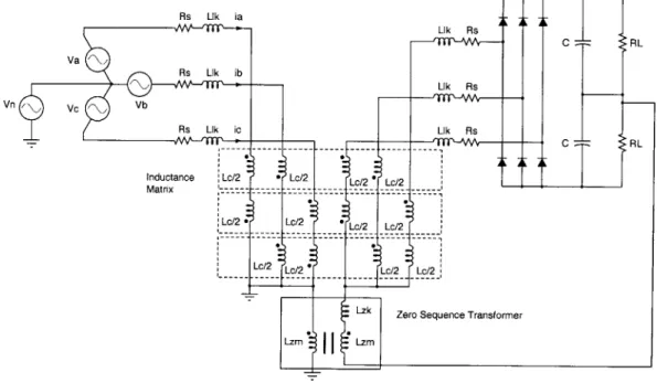
side open-circuit inductances, respectively, and M is the mutual inductance between windings. The inductance matrix given by Equation 2.8 has been implemented in PSPICE as illus-trated in Figure 2.2. Rs Lik ia X - -LUk Rs Va "-b LUk Rs Vn r\,, Vc Vb Rs LUk ic _LUk _Rs ---Inductance Lc/2 Lc/2 L/2 L2 M atrix ---- - ---- - -- -- -- -/ - -- -- - -Lzke ---- Z ro n---r-ns-rm-Lc2 Lzm Lzm L/ C

T

RL C RL

Figure 2.2: In-circuit transformer model of the flux linkage between two identical stator windings wound in-hand. A zero sequence transformer is described in §2.3.2.

This coupling between phases can be implemented in SPICE by coupled inductor statements; Appendix A contains the SPICE deck as well as the schematic file for PSPICE. Note that in Figure 2.2, the negative coupling coefficients and subsequent negative inductances are captured in the winding polarity of the coupled inductors, which helps to illustrate a better physical

(26)

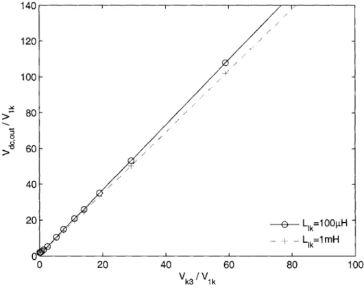
sense of what the parameter effects 140 120-1 03 CL 0 00 [ 80 60 40 20

flux is doing. Figure 2.3 illustrates on the system design.

20 40

V /V

how the model can be used to determine

60 80 100

Figure 2.3: Simulation result harmonic control function.

of the effect of a change on the series inductance in the 3rd

2.3 Zero Sequence Harmonic Control in Three Phase

Systems

By introducing one or more triple-n harmonics into the drive voltage of a three-phase machine,

the rectified output voltage from grounded-wye windings can be controlled and subsequently regulated. To first-order, these triple-n harmonic voltages produce triple-n harmonic currents, and introduce negligible net torque on the rotor, effectively decoupling voltage regulation from drive.

The rectifiers in Figure 1.1 are designed to operate in the discontinuous conduction mode. In this case, rectifiers in winding 2 behave as peak detectors of the line-to-neutral voltages, with

~, 26 m -/ /e -/ -/ -/ LIk=100tH - LIk=1mH

(27)

Section 2.3 : Zero Sequence Harmonic Control in Three Phase Systems al N1 \ ==

\+V

N a2 Vc2 Vb2 + 2, + I+ C/2 TC/2 N a3 VO Vb3 + C/2 C/2 +

Figure 2.4: Multiple Stator Connections Driving Three-Phase Rectifiers.

Va1 In1 Ic1 in V2 + V3 ~,, 2 7 ,

(28)

the dc output voltage given by

V2 = Vk 1sin O, + Vk3 sin(30p + 03), (2.10)

where Vkl and Vk3 are the amplitudes of the fundamental and third harmonic inverter voltages, respectively,

#3

_{is the phase angle of the third harmonic relative to the fundamental and O,} is the phase angle where the drive voltage is at a maximum. The angle O, is given by the extremum relation for the drive voltage

dV

2

d = VkI cos Op + Vk3 cos(30p +

#3)

= 0, (2.11)

d9p

which unfortunately is transcendental.

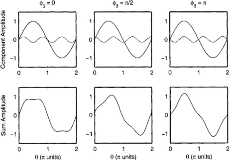
Figures 2.6 and 2.7 illustrates how the dc output voltage will vary with third harmonic amplitude and phase for a rectifier operating in discontinuous mode. One notices that for a third harmonic phase

#3

= 7r, the dc output voltage is not only monotonic, but also linear with

third harmonic voltage Vk3; the reason for this is immediately obvious from Figure 2.5, as the peaks of the fundamental and third harmonic occur coincidentally. While not proven, it can be plausibly argued that while V2 is monotonic with Vk3 over various intervals for different values

of 03, linearity as well as the widest range of Vk3 for monotonicity occurs only for

#3

7r.

3 0 33=T2 $3 a) 0 1 1 1 E E

0

a) 0 0. E -1 -1 -1 0 1 2 0 1 2 0 1 2 EQ0 ₀ 0 A E 0 1 2 0 12 0 12

0 (n units) 0 (n units) 0 (n units)

Figure 2.5: Drive Waveform with Third Harmonic

(29)

Section 2.3: Zero Sequence Harmonic Control in Three Phase Systems

3

-25

---01

V3N1 43 (n units)

Figure 2.6: Control surface for peak amplitude control using third harmonic voltage amplitude

(V3) and phase (#3) with fundamental voltage (V1i) held constant.

2.3.1 Voltage Output Control by Harmonic Amplitude Variation

The dc output V2 of a grounded wye-connected rectifier can be controlled by varying the third harmonic voltage applied to the primary drive winding in Figure 1.1. For 03 = 0, it can be exactly calculated (for a system that can be modeled as having no ac-side line inductance)

that V2 is monotonic with |Vk3| for |Vk3I > IVkil/6 (at IVk3I = IVkI/

6_{, IV21}₌

_VfIVkI/2).

_The

dependence of V2 on Vk3 is plotted in Figure 2.7(a) for values of

#3

between 0 and 7r. At03 = 7r,

V2 is affine for VUk > 0. At other value

#3

closed-form solutions to V2(Vk3) are likely to not

exist, but numerical methods can be used to estimate where this function is monotonic. Figure

2.7(b) shows that experimental data does indeed agree with calculations.

The strategy used for ir-phase harmonic control is founded on the fact that the peaks of the 3rd harmonic and the fundamental coincide. In this case, where we have assumed

discon-tinuous current in the phase connections of the secondary windings and 1:1 turns ratio, the dc output voltage will be very nearly equal to the sums of the peak voltages, Vkl + Vk3. In the implementation, a closed-loop PI controller ensures as Vkl drops, which for example is the case when the speed is lowered, that the 3rd harmonic Vk3 makes up the difference.

(30)

3 2.5-3 2 1.5--1C $3=0 -0.5 0 0.5 1 1.5 2 VkNk

(a) MATLAB Calculations

300 250 -S200 -- 150-I._a 100 0 10 20 30 40 50 80 70 80 90 10 150 too- 100---0- 13 0

o

10 20 30 40 50 60 70 80 90 100 Vk (RMS Volta) (b) Experimental Results[5]

Figure 2.7: Peak amplitude control using third harmonic voltage amplitude (V3) over a spread of phase (03) with fundamental voltage (V) held constant.

(31)

-Section 2.3 : Zero Sequence Harmonic Control in Three Phase Systems

(a) No 3rd Harmonic

(b) PI Control with Third Harmonic

Figure 2.8: PI Control of Dc Output Using Third Harmonic. The top trace shows V, the dc output of the grounded-wye secondary winding.

(32)

I1 12

Rs

Lis

Rs

Mo

Figure 2.9: T-Model for the Zero Sequence Circuit.

2.3.2 Zero Sequence Circuit

The zero sequence circuit is the portion of a multi-phase system where current can run in the same direction at the same time; it is that the part that is connected to one might call "common" to all the phases-with nomenclatures that include wye or neutral. Not all polyphase systems

have a zero sequence path, often systems that do are called wye-grounded.

Zero Sequence Reactance in a Three Phase Circuit

A key issue in driving a zero sequence current through two magnetically coupled windings with

grounded wyes is the effective magnetizing inductance, which is the phase-to-phase leakage in an induction machine, hence is typically kept as small as possible tfor good machine performance

[6]. Figure 2.9 shows a zero sequence circuit model for an induction machine with two identical

stators. Small magnetizing inductance Mo results in high zero sequence reactive current and represents additional loss in the stator resistance R8, as well as additional switch stress in the

power electronics.

One method to increase the zero sequence reactance is to decrease the phase-to-phase cou-pling. Looking for the moment at the flux from phase a of a three-legged transformer,

A L Lc Lcc,(.2

Aa = Lcia -

k

b - k

(2.12)

which implies that for a balanced set of currents with kp now less than unity, each leg must now support a higher volt-seconds, hence resulting in a larger core.

From this transformer picture of the inductance matrix, it becomes more obvious that the

(33)

Section 2.3 : Zero Sequence Harmonic Control in Three Phase Systems

amount of flux coupled to the secondary winding sorely depends on the coupling between the positive inductance windings (L,) being large (i.e. nearly unity ko3_{), yet with little coupling}

(kp) between adjacent phases (e.g. a and b). For a stator geometry with little saliency, which

is mostly the case with induction motors, the coupling between phases tends to be typically high. When viewed as the single-circuit T-model illustrated in Figure 2.9, this results in a zero sequence magnetizing inductance that is deplorably small; a zero sequence transformer in series with the neutral current path alleviates this problem with the caveat that it is now the zero sequence transformer that must transfer essentially all the zero sequence power to the secondary side.

Zero Sequence Transformer Topologies

One solution to the problem of small magnetizing inductance is shown in Figure 2.10, where a zero sequence transformer with an acceptable magnetizing inductance is used in the wye connection; a turns ratio other than unity offers an additional degree of freedom in optimizing machine design through the scaling of the zero sequence voltage and current. This zero se-quence transformer can be integrated into the machine back-iron, although this is not currently implemented. VC Va Vb 1:N Zero Sequence Transformer

Figure 2.10: Zero sequence transformer.

Power can be derived directly from the wye point as illustrated in Figure 2.11. In this topology, fewer rectifiers are required and a spit-capacitor ground is not needed; power to the output is derived solely from the zero sequence harmonics, so rectifier currents do not contribute to torque ripples, even without special accommodations in the control. Because the rectifiers only draw zero sequence current, standard field-oriented control schemes with fewer current sensors are more easily implemented.

3

ko = M/Lc for identical stator windings.

(34)

-1:N-

{

Figure 2.11: Direct zero sequence transformer.

Although using a direct zero sequence transformer offers a number of advantages, the trade-off is that all the dc output power is converted solely through a single-phase circuit, whereas the topology shown in Figure 2.10 allows, in certain regimes of operation, a portion of the power to be transferred to the output through the three phase circuit.

Under instances where the stator is not driven by an inverter, such as in an alternator, zero sequence harmonics can be exogenously driven through the wye as illustrated in Figure 2.12.

'field Va2 N₂

\

_;42 Vc2 Vb2+ vn,c C/2 V₂ ?-/ TC/2_

Figure 2.12: Exogenously driven zero sequence transformer.

2.4 Toward a Machine Design

Multi-use machines combine the challenges of both machine and transformer design. For exam-ple, in "standard" machines, insulation breakdown is a troublesome, but not a safety-critical

(35)

Section 2.4 : Toward a Machine Design

issue. In transformers where the primary is greater than some voltage threshold4

and where the secondary must be safe, the requirements for isolation (creepage and clearance) and insulation breakdown are strict and regulated by legislation.

While this section does not pretend to be a comprehensive treatise on the design of multi-use machines, nor does it suggest a design example, it attempts to offer some perspectives on the design limitations and advantages, which provides a motivation and some foundations for future work.

2.4.1 Fundamental Design Limitations

In the discussion of a machine design, there is an advantage to keeping the coupling between phases high, in very much the same way that a three-legged three phase transformer is better than three separate single phase transformers: the flux in each leg of the core has to carry only 1/2 of the flux than for each separate single phase transformer, resulting in a weight and volume savings for a given amount of apparent power.

2.4.2 _{Zero Sequence Control of Three-Phase, Three-Legged Transformer}

2.4.3 Scaling Laws

The rationale for a multiple output transformer (i.e. 1 : N : M : ... ) as opposed to multiple single transformers (i.e. 1 : N, 1 : M, ... ) appears to be two-fold. As power conversion is combined into a single piece of magnetics, both weight and volume is lower than the aggregate of the single transformers; per unit power handling capability along with better overall window utilization.

Area Product

The power handling capability of a transformer is proportional to the area product AP which is the product of the the window area Wa and the core cross-sectional area A

AP = WaAc. (2.13)

Both the weight and the volume of the transformer increase sub-linearly with Ap and hence also with power capability [7],

V Oc Ap. 75. _(2.14)

4

CE standards are 60V

(36)

Window Utilization

Isolation between primary and secondaries requires the use of a substantial amount of insulating tape between windings or the use of a triple-insulated wire5 to meet safety standards (e.g. CE and UL). With a lower power winding, the insulation consists of a higher percentage of the overall cross-sectional area of the wire. This results in a lower window utilization K for lower power windings. A poignant example of this is illustrated in Figure 2.13, where the insulation is a significant fraction of the wire section. Despite being a good fraction of the cross-section, the insulation is still much lighter than the enclosed copper so that the unit weight of the wire still increases pretty much linearly with its power handling capability.6

Induction Machine

In any case, when the voltage amplitude of the third harmonic is less than that of the funda-mental, there will be a fundamental component in the stator current and hence will contribute a torque ripple. However, one expects that a large fundamental drive voltage occur at high speed, where cogging is not as significant of an issue. At zero or low speed, rectifier current will be zero sequence. These have consequences in terms of per phase winding and core utilization.

5

Furukawa Tex-Eg.

6

The power handling capability of a wire is related to its temperature rise for a given amount of current, hence is inversely proportional to unit resistance. Because of that, the amount of power that a wire can handle is proportional to cross-sectional area, or to the square of its diameter.

(37)

0.4 0.6 0.8 1.0

Conductor Diameter (mm)

(a) Data plotted from Furukawa Tex-E6 wire table. [8]

% of Overall Diameter % of Cross-Sectional Area

0.4 0.6 0.8 1.0

Conductor Diameter (mm)

(b) Cross-Sectional Utilization

Figure 2.13: Better utilization of the wire cross-section by the conductor is unambiguous for larger diameters in triple insulated wire.

1.5

Section 2.4 : Toward a Machine Design

1.0

0.5

S4-I A

L

'

- Overall Wire Diameter

- - - Unit Weight 7.5 5 2.5 0 00.2 0 H 0 0 rJ~ 100 80 60 40 20 0 0 ~ 3 7

(38)

(39)

-Chapter 3

Vector Drive Control

The general concern of a variable speed drive is accurate and fast control of speed. However facetious as this sounds, it is not so straightforward of an endeavor in an induction machine. Speed and torque have no easy relation to voltage and terminal currents as on a dc machine. One must expend more effort to implement the classic speed control loop that has a minor loop for torque.

3.1 Constant Volts per Hertz Drive

In an induction machine with constant slip, flux is inversely proportional to frequency. For operation with constant flux, the ratio of voltage to frequency is held constant. At a given

flux, the maximum speed attained when the equivalent back-EMF equals the available inverter

voltage. At higher speeds, one must operate the machine at a constant voltage, while the flux decreases with speed: this is know as field-weakening or constant-power operation. The maximum available torque falls roughly in proportion to the inverse square of the frequency. [4] This type of drive is typically good for VSDs that generally operate in the steady and where the best transient performance is not required (e.g. HVACs operating under relatively constant load). In a closed-loop speed control system, response and its complement, disturbance rejection, is ultimately determine by the controllability of torque and hence flux. During a transient, neither constant slip, nor any value of slip is guaranteed with a constant V/Hz drive. In addition, at low speeds and high torques, the implied low voltage and high current means that voltage drops across the stator resistance become a serious limitation for a drive system whose control variable is terminal voltage.

While the advantage of constant V/Hz operation is that it is simple to implement and does not require current sensors except perhaps for fault detection, it is most likely not good enough

(40)

for traction and generation applications like EVs where speed and torque is both widely and strongly varying. Attempts at enhancing this method of speed controller include [9], but because of advancements in digital signal processors and subsequent price competitiveness, field oriented control methods have become more popular and accessible for high performance applications.

3.2 Indirect Field Oriented Control

Field oriented control takes advantage of the relation given by Equation 2.5

TM =p P(Aqridr -Adriqr)

to control the machine torque by specifying a flux and a current. If we set Aqr = 0 and hold Adr = Ao constant, then the torque is proportional to iqr, which resembles how the torque relates to terminal current in dc machine.

Aqr = 0 (3. 1a)

Adr = A0 Constant, (3.1b)

so the torque in Equation 2.5 can be written as

3

T

-

PAoiqr. (3.2)

2

Aqr = 0 implies that Aqr = 0 which results on the constraint in slip frequency WS--rrigr rrM .

s - - r - r. (3.3)

Adr Lar Adr Zq 33

The torque in stator coordinates is then given by

3r

=

-p Aoiqs (3.4)

2 Lar

An estimator for Adr can be derived from the first order differential equation

rr rrM

Adr

+ Adr = r . (3.5)

Lar Lartds

where Tr = Lar/rr is referred to as the rotor time constant. Adr can then be programmed by

(41)

Section 3.3 : Cartesian Feedback in the Synchronous Current Regulator

iqr _{through a first-order transfer function,}

A r _(3.6)

sTr + 1

Field-oriented control methods require the control of the current in the stator that is magnet-ically linked to the rotor. In a multiple stator machine, this current measurement is corrupted

by the additional loads presented by the secondary stators. This can be resolved by subtracting

those load components from the primary stator currents to get the drive currents, which is described in §3.3. The field-oriented system illustrated in Figure 3.3 includes an implementa-tion of a synchronous frame regulator. [10] gives a good discussion on tuning, stability and robustness of field-oriented controllers over parameter variations.

3.3 Cartesian Feedback in the Synchronous Current

Regulator

The advantage of regulating current in the synchronous frame of reference is that the stator currents are represented as dc. In RF parlance, this is the consequence of mixing down the sinusoidal ac currents in the stator terminals to a dc baseband. In this synchronous reference frame, zero steady state error can be achieved by placing a pole at the origin in the controller, i.e. integral control. In the stator reference frame, the currents are sinusoidal and hence cannot have zero steady error for a proportional-integral controller.1

By applying the conditions for field-oriented control in §3.2, the following state equations

can be derived for the direct and quadrature stator currents from the state equations for dAd/dt

and dAd,/dt:

dids m2

- Las _dddt _. -s W a- Lar qs - Vds (3.7a)

- (La

M 2 di

- Las - _ d_ = rsiqs + wLasids - Vqs. (3.7b)

Lar dt

It is apparent from Equation 3.7a that there is a strong coupling term between the direct

and quadrature axis currents that is proportional to the synchronous frequency.

A number of assumptions simplify the design of a controller for the Aardvark induction

machine. A key assumption in designing the synchronous current controller is that the electrical

'See Roberge[11] for a discussion on the error series derivation, which is germane to the tracking error of a proportional-integral controller to a sinusoid.

(42)

time constants of the machine are much smaller than the mechanical time constants. This is important because it allows us to satisfy the condition that the bandwidth of a minor loop be higher than the outer loop crossover frequency.

3.4 Integrator Anti-Windup

There are two output limits in any real inverter: current limit and voltage saturation (i.e. compliance of the current source). The maximum current that ought to be allowed depends on the physical limits of the power devices and the load. Voltage saturation is the result of a finite dc bus voltage, hence limiting the time rate of changes in flux (dA/dt). In the short-time scale, this is due to the time rate of change in current (di/dt), and on the longer time scale (or steady state) by winding resistances (stator and rotor) and to the time rate of change of mutual inductance, which is proportional to the speed w. Abstractly, by the product rule

dA di .dL

v - L

-

+ i . (3.8)

dt dt dt

Voltage saturation level is actually subtle: when one wants an inverter output with as few harmonics as possible, saturation occurs when the peak amplitude of the sine wave fundamental equals the one-half of the dc bus voltage for the half-bridge inverter (the full dc bus voltage for a full-bridge inverter); however, if over-modulation is allowed, the fundamental amplitude can be as high as 4/7r times larger by applying 100% duty cycle for 50% of the time, i.e. a symmetric square wave.

In terms of dq-axis quantities the current limit

is,max2 2ds + i qs2 (3.9)

The voltage saturation limit in this dq space

Vs,max2 Vds2 + Vqs2 (3.10)

From a control perspective, either limit presents itself as a classic actuator saturation. In a controller that integrates the error between the command (or reference) and the output, this error accumulates causing a large overshoot even when the actuator comes out of saturation and the setpoint been reached. That which is not a classical about this situation is the limitation of the magnitude of a vector of control variables (a MIMO system); a further complication is that the integrator in the controller is designed with an integrator for each variable so that there

(43)

-Section 3.4 : Integrator Anti-Windup

will be zero error in the steady state.

From Equation 3.4, ids programs the flux in the machine and iqs programs the torque. Typically, the flux is programmed to some optimal value below the rated motor speed; above this speed, the flux is decreased in inverse proportion to the speed, resulting in a constant power operating regime. If we assume that the speed changes at a much lower rate than the torque, the dynamics to consider in the controller design are that of the torque while that of the speed over the relevant time scale is invariant.

The condition for voltage saturation in Equation 3.10 allows for one degree of freedom, which we choose to be vd. In the polar coordinate frame, the contour is described by

0 = cos- 1 Vds (3.11)

Vs,max

This allows ids to still be programmed through Vds during saturation as illustrated in Figure

3.1.

In arranging the saturation conditions this way, we maintain the dc motor analogue, where the torque is constrained while the flux remains a free variable.2

The speed is also controlled by a PI controller, but it has SISO (single input, single output) dynamics, with an LTI function of the error commanding a torque, which we assume to be proportional to stator quadrature current sq,. The field, or flux is proportional to ids which value is determined by a field-weakening function of speed that we presume to have no dynamics.3 We would like to saturate the output of the controller for any of several reasons: a current limit given by Equation 3.9, a mechanical damage torque limit, and an electrical torque limit which depends on the flux4. The signaling of either these limits results in a relatively straightforward anti-windup strategy, such as limiting the speed-control integrator.

The current limit is the result of a number of factors. As already mentioned, these include a hard current limit to prevent physical damage and current source compliance due to a finite inverter voltage. Because the speed controller is much slower than the current controller, its integrator winds up at a much lower rate. We would like to signal a saturation from the current controller to the speed-control integrator only for longer time scale saturation events due to such things as demanding more torque than what is within the limits of the setting for the flux.

If the speed controller with its field-weakening algorithm and torque limits were ideal, these

longer time scale voltage saturation events would not occur; however, time-varying parameters 2

In a speed controller with field weakening, flux is a non-linear function of speed.

3

Only perhaps presumptuous in that the flux dynamics have a time scale in the neighborhood of the rotor time constant (Tr given in Equation 3.5), which we assume to be much smaller than the mechanical time constants.

4

The electrical torque limits can be precalculated from the flux.

(44)

Vqs,'tqs

I Vmax,'tmax

Vds itds

Figure 3.1: Contour of the saturation limit for the synchronous current regulator and the allowed trajectory in dq-space. There is a maximum torque limit that can also be described on the dq axis, but ought to be considered as part of the speed controller and not included in this diagram.

~NJ 44 m

J

(45)

Section 3.5 : Simulation

such as stator and rotor resistances, as well as nonlinearities in the iron permeability may well cause the speed controller to ask for more than the current regulator can provide.

The question is how does one determine the cause of the voltage saturation. Recall Equation

3.8. One way to do that is to keep track of the magnitude of the time derivative of the current di/dt during the voltage saturation. If

d

Fid1

[iqs] 2 (3.12)

where c is some threshold while the voltage is still saturated, then current controller signals a saturation event to the speed controller.

3.5 Simulation

Table 3.1: Aardvark Machine Parameters[2]

Stator Resistance Ra 2.OQ

Rotor Resistance R2 1.5Q

Stator Reactancet X1 2.8Q

Rotor Reactancet X2 2.8Q

Mutual ReactanceF XM 42.09Q

Free Moment of Inertia Jo 0.0168 kg - m2

The electrical parameters for the Aardvark induction machine are listed in Table 3.1. These parameters were derived by J. Holloway in [2] from a non-linear least square fit to the start up transient of the induction machine using IEEE blocked-rotor and no-load tests as well as impedance measurements for values for the initial guess.

The parameters in Table 3.1 along with an indirect field oriented controller and the strategies for anti-windup form the basis for a Simulink® model and simulation. Figure 3.2 predicts good transient performance under step speed reversals and steps in torque load. A diagram of the simulation can be found in Appendix C.

4

Reactances are customarily referenced to 60 Hz.

(46)

-C --5 400 200 -400-40 E 20 -- -. -.-.---- 2 0 - . -. .. - -- - -- - -- - ..- .

.-~-40

0 5 10 15 20 Time (seconds) (a) 0.6 - - - --0 .2 -- - - -- 0-S.8 06 0.2 0-0.1 -0.1 0 -0 5 10 Time (seconds) (c) 4. 10 -5 - -5-10 8 0 20 10 - - -- --10 - - - - - --$ 0 5 10 15 20 Time (seconds) (b) 10 0 -10 0-100 -50 400 200--200 - - - -0 5 10 Time (seconds) (d)

Figure 3.2: Simulation of induction motor under field-oriented control with speed and torque load steps. ~ 46 -^ 200 -0 200 -5 -- - - -- - - -- - -5

00

5 I

.

f is 20 15 20

(47)

Section 3.6 : Implementation

3.6 Implementation

The controller illustrated in Figure 3.3 is currently being implemented with minimal current

sensing as described in §4.4.2. There were a number of issues that precluded the inclusion

of results in this thesis. These included a number of hardware issues that included slow and erratic behavior in the opto-coupler circuit for the speed sensor and incorrect gains in the current sensing circuits. In the firmware, timing miscues in the field oriented control routine caused incorrect updates to the PWM routine.

A new opto-coupler circuit, as well as current sensing circuitry have been designed and

tested, but not yet integrated into the motor controller. Field-oriented control firmware is currently being debugged and results are forthcoming.

(48)

D - ids Parl~s

Tr TransformIC2

* Cntrlle toPolr p

e

P1 Contolle

+ + i nere

Sas r s transformetoe

Sare possible by proper scaling when subtracting the transformed stator winding currents. C-)

(49)

Chapter

4 Inverter Design

4.1 Power Module and Digital Signal Processor

A half-bridge inverter was designed around International Rectifier's PIIPM15P12DO07

pro-grammable isolated integrated power module. The power module contains the power electronics (e.g. IGBTs, gate drives, etc.), ac mains rectifiers, as well as a TI TMS320LF2406A DSP for digital control of the digital control of the motor drive and for any zero sequence control of dc output voltages.

The combined power electronic and control platform used in this thesis is shown in Figure 4.1. The PIIPM15P12DO07 from International Rectifier (IR) combines all the necessary power electronics (i.e. IGBTs, gate drives, and protection) with a TMS320LF2406A control-optimized

DSP from Texas Instruemnts, along with associated sensors, peripherals, auxiliary supplies, and

communications (e.g. RS485, JTAG, CAN). Although this platform has been discontinued by IR, it is close to an ideal model for the development of digital motor control systems.

4.2 Sine Wave Generation

4.2.1 Synchronous PWM

In variable speed drive, the inverter fundamental frequency varies with speed; in a field-oriented controller, it also varies with torque. When using a constant PWM frequency, non-integer ratios between the PWM frequency and the fundamental result in subharmonic content as a result of the "beating". Synchronous PWM was achieved by vaying the PWM switching frequency about a nominal (e.g. 10 kHz) so that the switching frequency is always a multiple n of the generated sine wave; an algorithm for hysteresis about the transition points of n was included

(50)

Power Module schematic:

Package:

L\ out I

ITN2 0 - R- Ou 2

Input bridge. brake and tlue phase inverter (BBI) with current PIIPM -BBI (EconoPack 2 outline compatible) sensing resistors on all output phases and thermistor

(a) PIIPM Integrated Power Module (b) PIIPM Schematic

PIIPM15P12DO07 System Block Schematic:

JIAG CAN -- resIstor 71 PflPM15P12WO7 out I BRK Conitol logicad

pmsw st$vply _{ACft4C minto}

Monatd onDSP f

---TM532ULF2406A)

R 2214 * qut lak. IGT * lOSTs

A dw dd and F * dFNs

Te p Power

C"Waa Seing ICS

(c) PIIPM Block Diagram

Figure 4.1: International Rectifier's Integrated Power Module[12]

(51)

Section 4.2 : Sine Wave Generation

to eliminate switching frequency jitter and oscillation. A good discussion of synchronous PWM can be found in [13].

4.2.2 Table-Based Implementation

A sine wave drive with low spurious harmonic content is important for rectifier output voltage

control. The three-phase inverter is based on a 108-element sine reference table that drives a symmetric PWM whose output is illustrated by the MATLAB plot in Figure 4.2. The size of the table was chosen to be both a multiple of 3 (aligned three-phase system) and 4 (quarter-wave symmetry). This results in a THD (total harmonic distortion) of 1.71% and a maximum error of 2.90%.

Table 4.1: THD and Maximum For a DLT Sine Reference Using Different Interpolating Func-tions

Interpolating Function THD

(%)

Maximum Error

(%)

ceiling(

)

3.37 5.81

floor( ) 3.37 5.81

round() 1.71 2.90

Although not implemented, an equivalent 27-element quarter-wave table could be used. The generation of the third harmonic is achieved by accessing every third table entry during each PWM update. A key to the generation of a sine wave with low harmonic content is the alignment of the PWM switching instances with the table element entries, which ensures synchronous PWM. A discussion of table-based implementations are presented in [14]. Figure 4.4 shows no harmonic content to at least 1.25 kHz with a 60 Hz fundamental and a third harmonic amplitude that is 50% of the fundamental. The algorithm is simple computationally because it performs only a direct table lookup and does not require interpolation. With this algorithm, the resolution for third harmonic phase modulation is determined by the size of the table. If a better resolution is required without the penalty of a large table size, interpolation for only the third harmonic lookup is required.

4.2.3 Parabolic Approximations

Real-time, on-the-fly second order approximations are a good alternative to look-up table based implementations. Angular resolution is limited only by the working precision of the desired number type. A second-order approximation requires at most three multiplications and three

(52)

1 0. -D 75 I-0 -0.25 -0.5 -0.75 -1 0 7r/ 2 7 r 0 (radians) 37r/2 27