Crop water stress under climate change uncertainty : global policy and regional risk

Crop Water Stress Under Climate Change Uncertainty:

Global Policy and Regional Risk

by

Arthur Gueneau

Submitted to the Technology and Policy Program, Engineering Systems Division

in partial fulfillment of the requirements for the degree of Master of Science in Technology and Policy

at the,

MASSACHUSETTS INSTITUTE OF TECHNOLOGY

September 2012

MA rNSTITUT

2

3

© Massachusetts Institute of Technology 2012. All rights reserved.

A uthor ...

Technologyand Polic Program, Engineering Systems Division July 25, 2012 Certified by

C. Adam Schlosser

Principal Research Scientist, MIT Joint Program on the Science and Policy

I

x

I

r2

1, Environmental, and Architectural

Engineering, University of Colorado at Boulder Thesis Reader

Accepted by... ...

Joel C. Clark Professor of Materials Systems and Engineering Systems Acting Director, Technology and Policy Program

Crop Water Stress Under Climate Change Uncertainty: Global Policy

and Regional Risk

by

Arthur Gueneau

Submitted to the Technology and Policy Program, Engineering Systems Division on July 25, 2012, in partial fulfillment of the

requirements for the degree of Master of Science in Technology and Policy

Abstract

Fourty percent of all crops grown in the world today are grown using irrigation, and shift-ing precipitation patterns due to climate change are viewed as a major threat to food secu-rity. This thesis examines, in the framework of the MIT Integrated Global System Model, the potential impacts of climate change on crop water stress and the risk implications for policy makers due to underlying uncertainty in climate models. This thesis presents the Community Land Model - Agriculture module (CLM-AG) that models crop growth and water stress. It is a global generic crop model built in the framework of the Community Land Model and was evaluated for maize, cotton and spring wheat. A full climate model, the IGSM-CAM, was first used to force CLM-AG and show the regional disparity of the response to climate change. Some areas like the Midwest or Equatorial Africa benefit from the higher precipitations associated to climate change while others like Europe or Southern Africa see the irrigation need for crops increase. The effect of a mitigation policy appeared contrasted, as water-stress for some areas (including Europe and Africa) is increased if greenhouse gases emissions are limited while for other areas (Central Asia, United States) it is reduced. A second analysis was carried in Central Zambia using uncertainty ensembles. The ensembles demonstrate the notable extent of the uncertainty stemming from different climate sensitivities and different regional patterns in climate models. Crops are impacted differently but a consistent result is that climate mitigation policies reduce uncertainty in crop water stress, making it easier to plan for any anticipated future climate change. Thesis Supervisor: C. Adam Schlosser

Title: Principal Research Scientist, MIT Joint Program on the Science and Policy of Global Change

Thesis Reader: Kenneth M. Strzepek Title: Research Scientist, MIT JPSPGC

Professor Emeritus of Civil, Environmental, and Architectural Engineering, University of Colorado at Boulder

Acknowledgements

This thesis would not have been possible without the help of many people at MIT and beyond.

First and foremost I want to thank my supervisor C. Adam Schlosser for his continued and friendly support, his valuable insights and his patience with me. This thesis would not have existed without him.

I would also like to thank particularly Kenneth M. Strzepek for his encouragements, his

great mentoring and his invaluable advice on this thesis.

This work would not have been possible without a great support from all the faculty, staff and students at the MIT Joint Program on the Science and Policy of Global Change. I owe special thanks go to Erwan Monier, Xiang Gao, Elodie Blanc, Yongxia Cai, and Jake Jacoby who all contributed in some way to this study. Chas Fant developed the CliCrop model that is the basis for CLMAG and provided many valuable insights.

I also want to thank all my office mates at the Joint Program for their friendliness and their always challenging questions on my work. My thanks also go to my friends in Paris, Boston and beyond, especially the Polytechnique and TPP communities. Special thanks go to my Erie Street room-mates Paul, Fernando and Jan, for their support and all the good times spent together.

Last but not least, I want to thank my family, especially my parents and sister for send-ing me kind words of support from across the ocean and always believsend-ing in me. Finally, someone who will recognize herself deserves all my gratitude for her overall support, her amazingly precise reviews, her always pertinent questions and everything else.

The author also gratefully acknowledges financial support for this work provided by the MIT Joint Program on the Science and Policy of Global Change through a consor-tium of industrial sponsors and Federal grants. Development of the IGSM applied in this research was supported by the U.S. Department of Energy, Office of Science (DE-FG02-94ER61937); the U.S. Environmental Protection Agency, EPRI, and other U.S. government agencies and a consortium of 40 industrial and foundation sponsors. For a complete list see http://globalchange.mit.edu/sponsors/current.html.

Contents

1 Introduction ₁₉

1.1 _{Background . . . 19}

1.1.1 _{The Challenge of Feeding Nine Billion People on a Finite Planet . . 19}

1.1.2 The Importance of Irrigation . . . 20

1.2 Contributions . . . 21

1.2.1 Main Questions and Approaches . . . 21

1.2.2 Outline . . . 23

2 Literature Review 25 2.1 _{Impacts of Climate Change on Agriculture . . . 25}

2.1.1 Direct Effects of Climate Change . . . 26

2.1.2 _{Indirect Effects of Climate Change Mitigation Strategies . . . 28}

2.2 _{Crop Models . . . 29}

2.2.1 Process-Based Crop Models . . . 30

2.2.2 Agroclimatic Indices and Production Functions . . . 31

2.2.3 Economic Models . . . 32

2.3 Uncertainty . . . 32

2.3.1 _{Economic Uncertainty . . . 33}

2.3.2 _{Climate Uncertainty . . . 33}

2.3.3 Crop Models Uncertainty . . . 34

3 The CLM-AG model 35 3.1 A Process-Based Model for Global Change Studies . . . 35

3.1.1 The IGSM Framework . . . .

3.1.2 Philosophy of the Model and Inspiration .

3.2 Description of the Model . . . . 3.2.1 Structure in CLM . . . .

3.2.2 Crop Physiology . . . .

3.2.3 Biogeophysics and Hydrology . . . . 3.2.4 Irrigation Need and Yield Reduction . . .

3.3 Model Evaluation: Historic Runs . . . . 3.3.1 Input Data and Method for the Evaluation

3.3.2 Results and Comparison with GAEZ . . .

3.3.3 Evaluation for the USA with FRIS . . . .

4 Irrigation in 2050 -A Global Perspective in an Integrated Framework

4.1 Datasets . . . . 4.1.1 Climate Data . . . . 4.1.2 Crop Data . . . .

4.2 Results . . . . 4.2.1 Evaluation of CAM versus NCC . . . . 4.2.2 Future Runs and Impacts of Policy . . . . 4.3 Analysis and Policy Implications . . . . 4.3.1 Main Findings and Analysis . . . . 4.3.2 Limitations of the Study . . . .

5 Climate Change Uncertainty: a Regional Study in the Zambezi River Valley 5.1 Motivation and Model . . . .

5.1.1 Central Zambia in the Zambezi River Valley . . . .

5.1.2 Climate Data and Uncertainty Quantification . . . .

5.1.3 Crop Data . . . .

5.2 Results . . . . 5.2.1 Distribution of Temperatures and Precipitations . . . .

5.2.2 Irrigation Need for Maize . . . .

. . . 3 5 . . . 37 . . . 3 8 . . . 3 8 . . . . 39 .. . . . 45 . . . 4 6 . . . 4 8 . . . 4 9 . . . 50 . . . 5 3 57 . . . . 57 . . . . 57 . . . . 58 . . . . 59 . . . . 59 . . . . 62 . . . . 76 . . . . 76 . . . . 77 81 81 81 82 88 88 89 94

5.2.3 Water-Stress Yield Reduction for Wheat . . . 96

5.2.4 Irrigation Need for Cotton . . . 98

5.3 Analysis and Policy Recommendations . . . 100

5.3.1 Use of Probability Distributions in a Policy-Making Environment . 100 5.3.2 Policy Implications . . . 104

5.3.3 Limitations and Use of the Model . . . 106

6 Conclusion 109 6.1 Key Findings and Policy Implications . . . 109

6.1.1 Global Findings . . . 109

6.1.2 Findings in Central Zambia . . . 111

6.2 Future Research . . . 112

A Crop Parameters 123 B Evaluation of CLM-AG versus GAEZ for Cotton and Spring Wheat 125 B.1 Cotton . . . 125

List of Figures

1-1 FAO Food Price Index, 1961 -2010 ... 20

2-1 Increase in global agricultural production. . . . 26

3-1 _{The IGSM Framework . . . 36}

3-2 The WRS framework. . . . 37

3-3 The CLM-AG structure . . . 39

3-4 CLM-AG plant physiology . . . 41

3-5 The biophysical and hydrological processes simulated in the Community Land M odel . . . 45

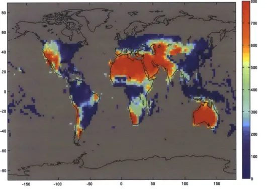
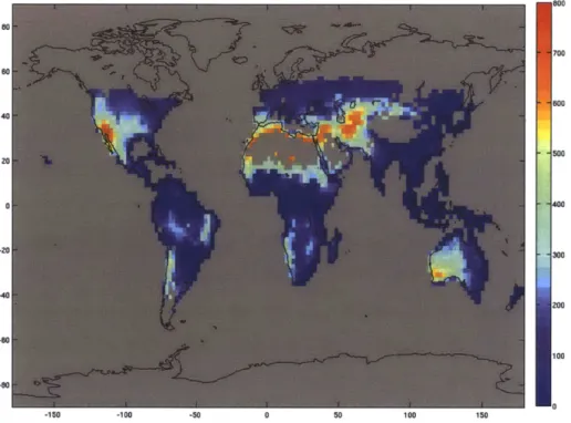
3-6 CLM-AG historic irrigation need for maize with NCC . . . 51

3-7 GAEZ historic irrigation need for maize . . . 51

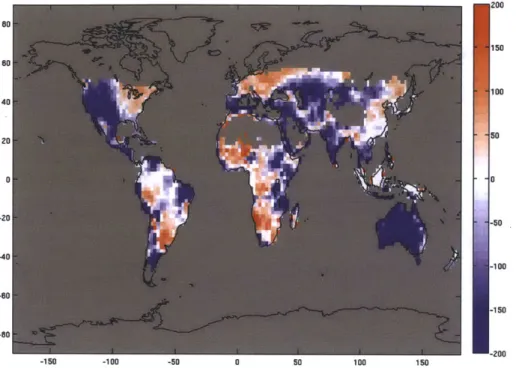
3-8 Comparison of maize irrigation need between CLM-AG and GAEZ . . . . 52

4-1 CLM-AG water deficit for irrigated maize - Historic IGSM-CAM run . . . 60

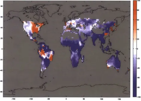
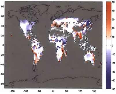
4-2 Comparison between historic IGSM-CAM and NCC runs of CLM-AG -Absolute difference . . . 61

4-3 Comparison between historic IGSM-CAM and NCC runs of CLM-AG -Relative difference . . . 61

4-4 Absolute change in irrigated maize irrigation need, UCE with CAM . . . . 63

4-5 Relative change in irrigated maize irrigation need, UCE with CAM . . . 63

4-6 Absolute change in irrigated maize irrigation need, L2S with CAM . . . 64

4-8 Absolute difference in irrigated maize irrigation need, L2S vs UCE with

CAM ... ... ... 66

4-9 Relative difference in irrigated maize irrigation need, L2S vs UCE with CAM 66 4-10 Relative change in rainfed wheat yield, UCE with CAM . . . 68 4-11 Relative change in rainfed wheat yield, L2S with CAM . . . 68 4-12 Relative difference in rainfed wheat yield, L2S vs UCE with CAM . . . 70

4-13 Absolute change in irrigated cotton irrigation need, UCE with CAM . . . . 72

4-14 Relative change in irrigated cotton irrigation need, UCE with CAM . . . 72 4-15 Absolute change in irrigated cotton irrigation need, L2S with CAM . . . 73 4-16 Relative change in irrigated cotton irrigation need, L2S with CAM . . . 73 4-17 Absolute difference in irrigated cotton irrigation need, L2S vs UCE with

CAM ... ... 75

4-18 Relative difference in irrigated cotton irrigation need, L2S vs UCE with CAM 75 4-19 Relative changes in precipitation (in percent) for the period 2090-2099,

relative to 1980-1999 - AR4 models average for the A1B scenario . . . 79

5-1 Map of the Zambezi River Valley and Central Province of Zambia . . . 82 5-2 Representation of the 400 run ensemble of the IGSM in the probability

space of climate sensitivity and rate of ocean heat uptake . . . 84

5-3 Schematic of the HFD hybridization technique . . . 85

5-4 Probability function of the distribution of annual temperature change in central Zambia. . . . 89

5-5 Cumulative probability of the distribution of annual temperature change in

central Zambia. . . . 90

5-6 Probability function of the distribution of annual precipitation change in

central Zambia. . . . 91

5-7 Cumulative probability function of the distribution of annual precipitation

change in central Zambia. . . . 91

5-8 Probability function of the distribution of OND precipitation change in

5-9 Probability function of the distribution of JFM precipitation change in

cen-tral Zam bia. . . . 93

5-10 Probability function of the distribution of irrigation need change for maize

in central Zambia. . . . 95

5-11 Cumulative probability function of the distribution of irrigation need change

for maize in central Zambia. . . . 95

5-12 Cumulative probability function of the distribution of yield change due to

water-stress for wheat in central Zambia. . . . 97

5-13 Cumulative probability function of the distribution of yield change due to

water-stress for wheat in central Zambia. . . . 97 5-14 Probability function of the distribution of irrigation need change for cotton

in central Zambia. . . . 99

5-15 Cumulative probability function of the distribution of irrigation need change

for cotton in central Zambia. . . . 99

5-16 Box diagram of the distribution of irrigation need change for maize in

cen-tral Zam bia. . . . 103

5-17 Box diagram of the distribution of irrigation need change for cotton in

cen-tral Zam bia. . . . 103

5-18 Box diagram of the distribution of yield change for wheat in central Zambia. 104

B-i CLM-AG water deficit (in mm) for irrigated cotton . . . 125 B-2 CLM-AG water deficit (in mm) for irrigated cotton . . . 126 B-3 Difference in water deficit estimates (in mm) for irrigated cotton between

CLM-AG and GAEZ . . . ..126

B-4 CLM-AG water deficit (in mm) for rainfed spring wheat . . . 127 B-5 GAEZ water deficit (in mm) for rainfed spring wheat . . . 128 B-6 Difference in water deficit estimates (in mm) for rainfed spring wheat

List of Tables

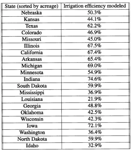
3.1 Irrigation Efficiency for Maize in the United States drawn from CLM-AG results and FRIS data. . . . 54

4.1 Changes in irrigation need between 2050 and 2000 under an UCE scenario for the major corn producing regions with irrigation. . . . 65 4.2 Changes in irrigation need between 2050 and 2000 under a L2S scenario

for the major corn producing regions with irrigation. . . . 65 4.3 Changes in irrigation need in 2050 between a L2S and a UCE scenario for

the major corn producing regions where irrigation is present. . . . 67 4.4 Changes in rainfed yield between 2050 and 2000 under an UCE scenario

for the major regions producing spring wheat. . . . 69

4.5 Changes in rainfed yield between 2050 and 2000 under a L2S scenario for

the major regions producing spring wheat. . . . 69 4.6 Changes in rainfed yield between 2050 and 2000 under a L2S scenario for

the major regions producing spring wheat. . . . 70 4.7 Irrigation need changes between 2050 and 2000 under a UCE scenario for

the major cotton producing regions where irrigation is present. . . . 74 4.8 Irrigation need changes between 2050 and 2000 under a L2S scenario for

the major cotton producing regions where irrigation is present. . . . 74 4.9 Irrigation need changes between 2050 and 2000 under a L2S scenario for

the major cotton producing regions where irrigation is present. . . . 76

List of Abbreviations and Acronyms

AOGCM Atmospheric and Oceanic Global Climate Model

AR4 IPCC Fourth Assessment Report

CAM Community Atmosphere Model CCSM Community Climate System Model CGE Computable General Equilibrium

CLM Community Land Model

CLMAG Community Land Model -Agriculture module

CRU Climate Research Unit, University of East Anglia DSSAT Decision Support System for Agrotechnology Transfer

EPIC Erosion-Productivity Impact Calculator EPPA Emission Prediction and Policy Analysis

FAO Food and Agriculture Organization, Rome GAEZ Global Agro-Ecological Zones

GDD Growing Degree Days GDP Gross Domestic Product

HFD Hybridized Frequency Distribution

IGSM Integrated Global System Model

IIASA International Institute for Applied Systems Analysis, Vienna LiS Level 1 Stabilization scenario

L2S Level 2 Stabilization scenario

LAI Leaf Area Index

MIT Massachusetts Institute of Technology, Cambridge, MA

NCAR National Center for Atmospheric Research, Boulder, CO NCC NCEP/NCAR Corrected by CRU

NCEP National Centers for Environmental Prediction, Camp Springs, MD

PFT Plant functional Type

ppm parts per million

SRES Special Report Emission Scenarios

SST Sea-Surface Temperature

UCE Unconstrained Emissions Scenario

UNFCC United Nations Framework Convention on Climate Change

WBM Water Basin Module

Chapter 1

Introduction

1.1

Background

1.1.1

The Challenge of Feeding Nine Billion People on a Finite Planet

With the global population projected to reach nine billion by 2050 (UN, 2004) and eco-nomic growth transforming the lives of millions in developing countries, world food de-mand is expected to roughly double by 2050 (FAO, 2009). This includes a westernization of diets in lower-income countries, where energy-, land- and water-intensive meat demand is expected to increase significantly. Agriculture already uses 34% of ice-free land world-wide (Ramankutty et al., 2008) and is responsible for 10 to 12% of direct global greenhouse gases emissions' (Smith et al., 2007), including most of the global emissions of methane. Humans used about 54% of all attainable runoff in 1996 (Postel et al., 1996). Of this amount, 87% is used for agriculture, mostly for irrigation purposes (Shiklomanov, 2000).

Despite its footprint on the environment, food production is essential for human sub-sistence. As shown in Figure 1-1, after declining through the last quarter of the twentieth century, largely due to the Green Revolution and an unusually mild climate (Ziska, 2011), food prices have started to rise again, and it is estimated that in 2011 six hundred million people in developing countries are still undernourished (FAO, 2011). The double concern

'This number would be higher if we were to take into account indirect emissions due to deforestation to claim new crop land or pastureland, which is much harder to quantify.

Index (2002-04 = 100) 400 350 300 250 200 150 100 50 0 ... 1961 1968 1975 1982 1989 1996 2003 2010

Figure 1-1: FAO Food Price Index, adjusted for inflation, 1961 - 2010, calculated using international prices for cereals, oilseeds, meats, and dairy and sugar products (FAO, 2011). of environmental stress caused by agriculture and of the absolute necessity of producing enough food for humans makes feeding the planet sustainably one of the biggest challenges of the twenty-first century 2.

1.1.2 The Importance of Irrigation

In the broader context of food security, irrigation is an often overlooked but nevertheless important issue. Indeed, even if irrigated land composes only 20% of the cultivated area globally, it accounts for around 40% of the global food production (D611, 2002). As is shown on the map of irrigated areas worldwide presented in Siebert et al. (2005) irrigation is crucial for food production in certain countries like Egypt, Pakistan or India. Any drop in irrigation capacity, whether from increased water demand from crops or decreased runoff in the streams would have dire consequences for these countries, especially at the time they need to ramp up their production capacity to meet the demands of a growing population. At the same time, the development of irrigation in some areas (mostly in Africa) could spur

2

The interested reader can find a more extensive presentation of these issues in a TED talk given by Professor Jonathan Foley from University of Minnesota (Foley, 2010).

an agricultural revolution in these countries and increase crop yields, thus improving food security and being part of the answer to meeting food demand growth.

Irrigation is crucial to the agricultural policies of many countries but evaluating the relevance of irrigation projects becomes increasingly difficult as climate changes. Indeed, one of the major factors relevant to assess the potential success of such a project is the amount of water required by crops to grow healthily. However this irrigation need is highly dependent on temperature and on precipitation, and is likely to vary significantly under a changed climate.

Thus tools are needed to assess the potential impact of climate change and its surround-ing uncertainty to help policy makers make informed decisions on irrigation projects and, more broadly, to assess the risks future climate change could pose on human food supplies. The potential impacts of climate change on irrigation need for crops and the uncertainties policy makers must take into account when dealing with these issues are the subject of this master's thesis.

1.2 Contributions

1.2.1

Main Questions and Approaches

The issues that have been outlined in the previous section give rise to many interesting questions. We will concentrate on the following issues:

- Which areas in the world could face the largest changes in irrigation need by the middle of the century? What would be the impact of mitigation policies on this outcome? Would agricultural production be better or worse off in a warmer world, from a water stress point of view?

- How can we efficiently characterize irrigation need uncertainty at the regional level? What are the relevant tools we can provide policy makers to help them make informed decisions on irrigation projects whose success are dependent on a potential change in climate? Do global climate policies have an impact on irrigation at the local level?

As it is impossible to rely on past observations to predict future irrigation need - given climate change and its impact on the planet - we must rely on models to answer these questions. For this work, a crop and irrigation model called the Community Land Model

-Agriculture module (CLM-AG) has been developed. This model was designed to be a part of the MIT Integrated Global System Model (IGSM) framework (Prinn et al., 1999; Sokolov et al., 2005). This integrated approach ensures that all models parameters and results (from greenhouse gases emissions to irrigation need) are consistent with one another

and do not result in physical impossibilities.

To answer the first question we use the results of a full 3-D climate model, the IGSM

-Community Atmosphere Model (IGSM-CAM, Monier et al. (2012)) driven by the emis-sions scenarios from the MIT Emission Prediction and Policy Analysis (EPPA, Paltsev

et al. (2005)) model. We then compare the average irrigation need modeled for the period

1980-2000 with what the model predict for the period 2040-2060. Two distinct scenarios

were considered for the future runs: an unconstrained emissions scenario and a climate change mitigation scenario. This allows us to draw conclusions on the different regional impacts of climate change and on the potential impact of a mitigation policy on irrigation need.

To answer the second question, we focus on the Central Province of Zambia in South-Western Africa and take advantage of the IGSM functionality to run uncertainty scenarios. For each emissions scenario, the hybridization of a statistically representative ensemble of 400 IGSM 2-D model runs with AR4 kernels for regional impacts (Schlosser et al., 2011) leads to a distribution of 6800 possible outcomes. We reduce this distribution to approximately 400 weighted outcomes using a Gaussian Quadrature reduction technique (Arndt, 1996). CLM-AG allows us to characterize the impact of these different scenarios on crop irrigation need and to build probability distribution of the evolution of crop water stress by 2050 in the Central Province of Zambia under the two emissions scenarios.

1.2.2

Outline

Chapter 2 reviews the existing literature on the impacts of climate change on agriculture, on the models that have been used to make these assessments, and on the underlying un-certainties.

Chapter 3 describes the crop and irrigation model called CLM-AG that was developed for this study. We also present in this chapter two different evaluations of CLM-AG. The first one compares CLM-AG to another crop model, the IIASA-FAO Global Agro-Ecological Zones (GAEZ, Fischer et al. (2012)). The second one compares a subset of the model for the United States to the water withdrawn for irrigation of maize as reported in the Farm and Ranch Irrigation Survey conducted by the US Department of Agriculture

(USDA, 2008).

Chapter 4 shows the results of the global study using the IGSM-CAM forcing under two different scenarios: an unconstrained emissions scenario and a scenario where policies limit the concentration of carbon dioxide to 550 ppm by the end of the century. We then identify the impacts of these two policies on major growing areas of corn, wheat and cotton globally and conclude on some of the impacts of a mitigation policy on irrigation as well as on the regional patterns of change.

Chapter 5 then presents the results of the regional analysis carried out for the Central Province of Zambia. We analyze the distribution of the possible outcomes for irrigation need under two different scenarios and provide a few tools to evaluate them and interpret the results in a policy making framework.

We finally summarize the main findings of this work in Chapter 6 and discuss future research that the development of CLM-AG renders possible.

Chapter 2

Literature Review

This chapter reviews relevant literature in the field. Section 2.1 focuses on the effects of climate change on agriculture and crop production. Section 2.2 describes the different varieties of crop models that have been developed to study the impacts of climate change on agriculture. It assesses the strengths and weaknesses of each model and focuses particularly on irrigation models. Finally, Section 2.3 reviews the major uncertainties a modeler is faced with when developing an assessment tool for future agricultural production.

2.1

Impacts of Climate Change on Agriculture

The twentieth century has been characterized by a constant increase in agricultural produc-tion driven by the use of new varieties and the development of fertilizers (Figure 2-1). This has been widely referred as the Green Revolution. It has helped keep food prices at a his-torically low level. However, the Green Revolution occurred during a time of remarkable climate stability (Swanson et al., 2009). Will agricultural production be able to continue rising in the coming years under a changing climate? As most of the existing science is compiled in chapter 8 of the working group II report for the International Panel on Climate Change (Smith et al., 2007) we only review the main findings here and highlight what can be explored with CLM-AG.

Global Agricultural Production

Figure 2-1: Increase in global agricultural production. Data source: USDA.

2.1.1 Direct Effects of Climate Change

Water

Crops require water to grow. Currently, irrigated land represents 20 percent of cultivated land but 40 percent of total agricultural production (D611, 2002). The largest impact in the agricultural sector is likely to be felt in irrigation, as water supply becomes scarcer in some areas and more subject to extreme variations (Ziska, 2011). According to Do11

(2002), two-thirds of current globally irrigated areas will need more water by 2070, due to a combination of higher temperatures and lower precipitation. At the same time, water supply

- namely river runoff - is likely to decrease in some of these areas (Kundzewicz et al., 2007, 2008). According to a study by Fischer et al. (2007), mitigation could reduce globally the

impacts of climate change on annual agricultural water requirements by about 40 percent, or 125 to 160 billion m3 _{compared with an unconstrained emissions scenario. However, this}

study relies on a rather simple crop model and we aim at improving the results regionally

Temperature

Crops are very sensitive to temperature. Ziska (2011) provides a table of optimal flowering and vegetative stage temperatures for the main US crops (Table 2.2 in the cited volume). Under climate change it is likely that temperature will frequently exceed the optimal range for crops, leading to reduced yields or a need to develop new hybrids. The main finding is that crop response to temperature is not linear, as shown in Schlenker and Roberts (2009). These non-linearities are not implemented in CLM-AG (discussed in Chapter 3) as new hybrids better adapted to a warmer climate may appear. Nevertheless, temperature indi-rectly affects the water requirement from the crop as a warmer weather means a higher evapotranspiration from the plant, which CLM-AG takes into account.

Extremes

Under any climate change (i.e. human or natural), extreme weather events are likely to become more frequent and/or more intense, for temperatures and precipitation alike (IPCC, 2012). The most impactive of extreme events to agriculture are droughts and floods, as well as heat waves. These extreme events can dramatically reduce crop yields when they occur during the most critical stages of crop growth and could impact overall agricultural production (Rosenzweig et al., 2001; Smith et al., 2007). As the intent of CLM-AG is to model irrigation, it does not model the direct impact of these events on crop physiology. It does, however, model the impact of a drought on irrigation demand and the associated yield reduction.

Change in Carbon Dioxide Concentration

Extensive studies have been conducted on the effect of increasing CO2 concentrations on

crop yields. Kimball et al. (1993) posits a yield increase of 30% under a doubled carbon dioxide concentration based on closed environment experimentations, but this rate is highly contested as the technique involves small volumes of air that may create micro-climatic ef-fects (Ziska and Bunce, 2007). It is thus very uncertain that this result would hold in a natural environment. It is clear that more research in this area is required before providing

a conclusive parameterization in this regard, thus this implementation of CLM-AG does not directly take carbon dioxide concentrations into account when modeling the plant

physiol-ogy.

Nutritional Value

Rising levels of carbon dioxide in the atmosphere also impact the physiology of the plant through different mechanisms (more efficient nitrogen uptake, stomatal closure, etc.). Taub

et al. (2008) estimate experimentally that crop nutritional value could decrease as much

as 15% if the concentration of CO2 in the atmosphere doubles. Loladze (2002) shows

that rising carbon dioxide could also reduce the quantity of essential micronutrients in the plants, such as iron, iodine and zinc. These findings have strong implications for the quantity of food that needs to be grown to feed the planet; however, they do not impact directly crop water requirements and are not considered in this implementation of

CLM-AG.

2.1.2 Indirect Effects of Climate Change Mitigation Strategies

Fertilizer Price

Synthetic fertilizers are overwhelmingly produced from natural gas. As of 2003, fertilizer production was consuming approximately 1.2% of the world's energy and was responsi-ble for approximately 1.2% of total greenhouse gases emissions (Kongshaug and Jenssen,

2003). Hence any climate policy that prices directly or indirectly emissions (like a carbon

tax or a cap-and-trade policy) will increase fertilizer price, decrease fertilizer use and there-fore impact global agricultural production. Irrigation can potentially offset the amount of fertilizer needed to improve yields and is consequently an important tool for mitigating the impacts of such a climate policy.

Biofuels

Some politicians (see the US Energy Policy Act of 2005 and the EU Directive 2003/30/EC) and scientists (Demirbas, 2009) have championed replacing conventional fossil fuels with

biofuels as a way to green the transportation sector. However, Melillo et al. (2009) showed that the introduction of biofuels created unintended consequences for agricultural produc-tion. By shifting some of the best land from agricultural production to fuel production (as biofuel prices as likely to be higher than food prices), it relegates food production to less fertile land. This would either reduce yields, require an intensification of the production through the use of more fertilizers, or require more irrigation because food production is displaced to marginal land. As a consequence, biofuels are generally seen as a threat to food security (Rosegrant et al., 2008b; Boddiger, 2007). Though it is not the focus of this work,

CLM-AG would allow us to explore in future works the impacts of such a displacement of

food production on the irrigation need and on the water systems of countries.

2.2

Crop Models

Farm production is influenced by biophysical conditions (temperature, rainfall, soil, pests, etc.) and by the socio-economical context (population, lifestyle, income, water resources, etc.) Farmers respond to these external conditions through management decisions (crop choice, irrigation, fertilizer use, etc.) The variety of parameters that influence a crop and the high adaptivity of farmers makes modeling crops a very difficult task. Moreover, inputs range from the local (soil, precipitation) to the regional (water resources, subsidies) or even the global (carbon dioxide concentration, food prices), and all need to be taken into account if one wants to reliably model food production.

As a result this system is too complex to be studied in its entirety. First, experiments to study the impact of climate change on food production are not possible. Thus, research has to rely on models to analyze potential effects. Second, as one cannot model the system in its entirety, different models perform different types of assessments at different scales.

There are three general types of crop models: process-based models, statistical mod-els and economic modmod-els. We describe all of them below, but focus more extensively on process-based crop models as CLM-AG falls into this category.

2.2.1

Process-Based Crop Models

Process-based crop models are usually deterministic. Any change in the model results is due to input data or parametrization. Most of these models consist of three modules: a soil module with water infiltration from precipitation or irrigation, a plant module to represent the growth and physiology of the plant, and a canopy air-space module to simulate evaporation and transpiration. They are usually based on a numerical integration over a rather short period of time that can range from hours to a month (Faivre et al., 2009). These models are all data-intensive but they can capture non-linear responses to climate change (Challinor et al., 2003).

DSSAT

The Decision Support System for Agrotechnology Transfer model (DSSAT, Jones et al.

(2003)) was developed to provide farmers with a way to predict the response of their crops

to different management options such as fertilizer use or irrigation. It is very detailed and has been developed for as many as twenty different crops. It focuses on fertilizer use and plant processes. In climate change studies it has been used to see how crop management might evolve under a changing climate (e.g. Rosenzweig et al. (1994)) or for local studies on specific crops (Guerefia et al., 2001; Brumbelow and Georgakakos, 2001)). Arguably the most detailed of crop models, it nevertheless requires a large amount of data. Fur-ther, its very detailed parametrization becomes problematic at a global scale as field data aggregation for inputs can lead to large errors.

EPIC

The Erosion-Productivity Impact Calculator (EPIC, Williams and Singh (1995)) is primar-ily a soil hydrology model. It was developed to track the impacts of erosion and soil productivity on crops. Stockle et al. (1992) modified the model by adding a carbon dioxide function for climate change assessments. It has been used since in a number of such climate assessments (Izaurralde et al., 2003; Tan and Shibasaki, 2003; Easterling et al., 1996). It is also a field-scale model that requires a number of local parameter inputs and therefore

becomes parametric intensive on a global scale.

The FAO models: CROPWAT and AquaCrop

CROPWAT (Smith, 1992) is an empirical process-based crop model. In contrast to the

preceding models it has the advantage of being generic and requiring very little input pa-rameters for the plant or soil specifications. Conversely, this results in a somewhat larger uncertainty in the outputs. It has been used for local studies of the impact of climate change on irrigation resources (Rodriguez Diaz et al., 2007; Rosenzweig et al., 2004) or on rainfed agriculture (Moussa and Amadou, 2006).

AquaCrop (Steduto et al., 2009; Raes et al., 2009) is the evolution of CROPWAT. It is also a process-based model, focused on evaluating the irrigation need for crops. As it was developed and released only recently, and is parametrized for relatively few crops, only a few studies have used it (e.g. Chung (2010)). AquaCrop simulates crop growth over the season, and tracks a variety of different stresses to the crop (heat, water or nutrient shortage, soil salinity, etc.) and hydrological processes in the ground. As a result, it outputs a variety of indicators including yield and water deficit.

CLM-AG is directly inspired by these models as its purpose is to be a global irrigation

model. However, only the water-deficit routines from AquaCrop were implemented as total yield is secondary to this study. It is, like CROPWAT and AquaCrop, a generic crop model and has been parametrized for corn, wheat and cotton, given the global agro-economic importance of these crops.

2.2.2

Agroclimatic Indices and Production Functions

Agroclimatic Indices

Agroclimatic indices are used to determine if a crop can be grown at a given place. They rely mostly on temperature, average rainfall and soil characteristics to compute the suit-ability of a given place for a given crop. Carter et al. (1996) at a local level or Fischer et al.

(2005) at a global level use this method to assess the potential shift of agricultural land and

practice adaptations and provides insights on climate impacts on crop localization; how-ever it does not compute actual yields and irrigation needs, except when coupled with a process-based model (Fischer et al., 2012).

Production Functions

Production function models are statistical models based on a regression of relevant factors that underly the yield of a crop. For example, these factors can include temperature, rainfall, sowing date and fertilizer use. They are mostly modeled after present-day systems and thus are a very unreliable estimate for future yields as regression coefficients are bound to change because of climate change and subsequent adaptations (Mearns et al., 1997). However, Parry et al. (2004) at a global level or Iglesias et al. (2000) at a local level have combined such models with precise process-based model runs of DSSAT (see 2.2.1) to calibrate the regressions in the future.

2.2.3

Economic Models

Economic models do not predict the irrigation need of crops as they lack a physical basis. Aside from macroeconomic models that incorporate results from a process-based model (Parry et al. (2004) for example), the main economic approach to modeling the impacts of climate change on the farm is the Ricardian method. This method uses statistical production functions to compute not a yield but the value of the land or the farm revenue. These outputs are in turn used to analyze the economic effects of climate change as in Mendelsohn et al. (1994).

2.3 Uncertainty

As it is the rule for any model, crop models are uncertain in nature and do not exactly represent reality. This is an even bigger problem when it is run in the future as there is a wide uncertainty surrounding climate models. The three major sources of uncertainty in the water stress predicted by any process-based crop model are the uncertainty in

green-house gases emissions, the uncertainty in the temperature and precipitation outputs from the climate model and the uncertainty in the computed crop water need from the crop model itself.

2.3.1

Economic Uncertainty

The largest input uncertainty in climate models comes from the uncertainty in greenhouse gases emissions (Stott and Kettleborough, 2002; Webster et al., 2002). Indeed these emis-sions depend largely on the future state of the economy and on the production techniques that will be chosen, as well as on eventual mitigation policies. One way to quantify the evolution of these emissions in the future is to use a Computable General Equilibrium

(CGE) model. One such model is the MIT Emission Prediction and Policy Analysis (EPPA)

model (Paltsev et al., 2005). In contrast to the IPCC Special Report Emission Scenarios (SRES, Nakicenovic et al. (2000)), using a CGE model ensures that emissions and eco-nomic growth are consistent with each other. However, as summarized in Abler et al.

(1999), there is wide uncertainty associated with CGE models outputs, even given a

par-ticular growth course, as most economic elasticities are highly uncertain. Webster et al.

(2008) provide a technique to quantify some of these uncertainties in the EPPA model.

2.3.2

Climate Uncertainty

Climate model uncertainties are well recognized and documented (Deser et al., 2012; Ran-dall et al., 2007). Three parameters summarize most of this climate models internal uncer-tainty: climate sensitivity, ocean uptake rate and aerosol forcing effect1_{. The uncertainty}

surrounding these parameters explains most of the prediction differences between climate models in terms of temperature increase.

One way to recognize this uncertainty is to create several runs of a given climate model while varying these parameters. Forest et al. (1999) describes a technique to select a

phys-1

The climate sensitivity can be defined as the ratio of temperature change to radiative forcing change in an equilibrium state, the ocean heat uptake rate is the amount of carbon absorbed by the oceans and the aerosol forcing is the impact of aerosols and clouds on the radiative forcing of the atmosphere. More complete definitions can be found in Sokolov et al. (2009).

ically possible subset of these parameters given the climate observations during the twen-tieth century. This is the approach that is used in the MIT Integrated Global System Model (Sokolov et al., 2005, 2009) to represent the underlying climate uncertainty.

Besides the uncertainty on the level of the climate response to an increased concen-tration of greenhouse gases, there is a large disagreement between the different climate models in terms of regional impacts of climate change. For example, some models pre-dict that precipitation could increase by 20% in the North-East United States while others predict that they could decrease by 20% (Christensen et al., 2007). Schlosser et al. (2011) describe a technique to take this regional uncertainty into account and describe a multi-model ensemble of climate forcings. We discuss this technique at length in Chapter 5.

2.3.3 Crop Models Uncertainty

Finally, there is a very high uncertainty associated with crop models themselves as crop growth depends on a large number of parameters (Monod et al., 2006). Different types of models face different issues.

A detailed model like DSSAT represents crops very precisely but in return require

ex-tensive input data. This data is usually not available at the global scale, and aggregation issues will arise.

On the contrary, a generic crop model like CLM-AG or AquaCrop does not simulate all the processes involved in crop growth. It is thus likely to be imprecise at the field level. However, at a global scale the model representation becomes more palatable as it does not require much data.

Although these uncertainties have an impact on the absolute water deficit the crop is facing, we argue later in this work that only differences in irrigation need from 2050 to the present are useful to policy makers. Indeed global model outputs need to be downscaled at a local level to generate relevant data for decision maker. This process requires changes in irrigation need (or water stress) and not the absolute values. Following the community, we contend that differences are much more reliable as they identify the impact of one factor only (here climate change).

Chapter 3

The CLM-AG model

In this chapter we describe the CLM-AG model. The chapter first explains the reasons for developing the model and the specifications the MIT Integrated Global System Model required it to have. Then we describe its structure and algorithms. Finally we present two different evaluations of the model on a historic run with past climate data.

3.1 A Process-Based Model for Global Change Studies

3.1.1

The IGSM Framework

The CLM-AG model has been developed with the potential to become a component the

MIT Integrated Global System Model (Prinn et al., 1999) that would be used for water and food studies under global change. In the context of an integrated global assessment, a crop water stress and irrigation demand model must meet certain specifications that differ from other crop models (yield prediction or irrigation planning at the field scale require different specifications for example). First the model needs to output a monthly irrigation demand (later used in the Water Basin Model in the IGSM framework) and a rainfed yield factor (that quantifies the effects of water stress on crop yields, and that is used in calculating the agricultural output). Second, as the model has to be global, it must be able to run on large grid cells and to be as computationally efficient as possible. Finally, as it is difficult to predict how crop characteristics will change in the future, this model needs to be a generic

crop model with a minimal set of inputs.

wgloaasear

E VE

---ATMOSPHERE URANanffan

2-D Dynamicadl, PhySical, Air Pollutonr t*"'Prtwearnf

anidCheical rcess Prova Iero"

sunltight Water c ycles, energy & mnomenitum trarnsffrsV050gvr

ar& $eaj temperature, C02, CH4, N20, nuf riernt- 00" as PF -0 ~pollutants, sotl properties, suir ace albedo, prouinee .

ea-te coverage Ocean COt upiaketa

land CO,, uptake, vegetation chanig... soil avt Vtative

carbonM net primary l I w c F LAN prodseivity,

franDr3 -D D ynnWate& Eoigy Budw b trace gas emissions frm eCosystems, Bloge cemia Process permafrost area...

Figure 3-1: The IGSM Framework.

Figure 3-1 describes the MIT Integrated Global System Model (IGSM) framework, with a particular highlight on the Water Resource System (WRS, Strzepek et al. (2010)). Using emission predictions and economic outputs from the MIT Emission Prediction and Policy Analysis (EPPA) model (Paltsev et al., 2005) and earth system modeling predic-tions from the IGSM (Sokolov et al., 2005), the Water Basin Module (WBM) describes climate impacts on water demand as described in Figure 3-2. Previously, the hydrology part (runoff) would come from the Community Land Model (CLM, Bonan et al. (2002)) and the agriculture part from CliCrop (Fant et al., 2012). These two distinct parts may create an inconsistency in the framework. Indeed, CLM and CliCrop did not have the same soil water calculation algorithms, leading to inconsistencies in their respective water balance when putting the results together in WBM. CLM-AG solves this issue by integrat-ing the two models with a sintegrat-ingle soil water module. It also integrates advances in crop modeling that were not simulated or simulated differently in CliCrop.

Emission Prediction and

Policy Analysis (EPPA)

GHG Emissions

Integrated Global

System Model (IGSM)

Climate data

Community Land Model

with Agriculture

module (CLMAG)

Hydrology Data Agriculture Data

Water Basin Model

(WBM)

Water Constraints to the Economy

Figure 3-2: The WRS framework.

3.1.2

Philosophy of the Model and Inspiration

CLM-AG was originally intended to be a simple implementation of CliCrop in the very flexible Community Land Model (CLM v3.5, Oleson et al. (2004) and Oleson et al. (2008))1. However, it evolved to include advances in modeling and a better understanding of

man-agement options for agriculture.

'The MIT Joint Program on the Science and Policy of Global Change currently uses the version 3.5 of CLM for most of its land studies.

As an evolution of CliCrop, CLM-AG relies on the same principles; the irrigation and yield reduction routines are taken from CROPWAT (Smith, 1992). However, the physiol-ogy of the crop needed to be more precise than the one in CROPWAT as CLM runs on an hourly time-scale (CROPWAT is monthly). CLM-AG thus relies primarily on AquaCrop physiology routines to drive plant growth (Raes et al., 2009). Meanwhile the soil hydrology remains unchanged from the original CLM model.

3.2 Description of the Model

We describe here only the agriculture and irrigation routines created during the course of this work. The interested reader will find a precise description of the other CLM routines in the CLM 3.0 technical description (Oleson et al., 2004) and the subsequent improvements of CLM 3.5 in the CLM 3.5 description (Oleson et al., 2008).

3.2.1

Structure in CLM

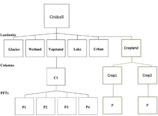
The CLM structure is a nested subgrid hierarchy under the unit of the gridcell. Climate inputs are given at the gridcell unit. Each gridcell is composed of multiple landunits, soil columns and Plant Functional Types (PFTs). Soil properties are defined at the landunit level. The energy and water balances are made at the column level. Of primary concern for agriculture, soil hydrology routines operate at this level. Finally, plant dynamics are simulated at the PFT level with both biophysical and biochemical routines.

Figure 3-3 shows the changes from the usual CLM structure made in CLM-AG. Crop-land is now a separate Crop-landunit with each crop being a distinct column. Separating crops in different columns (and not only PFTs) prevents them from competing for the same water resources present in the ground: two distinct fields are completely independent when it comes to the water content in the soil.

The scheme is entirely flexible and one can add new crops as needed. Currently, only maize, spring wheat and cotton are implemented in the framework as they are among the two most important food crops and cash crop, respectively. It is also important to note that besides the plant physiology, all other CLM routines (hydrology, energy and water

Figure 3-3: The CLM-AG structure. Changes to the usual CLM structure are represented in green. (Adapted from Oleson et al. (2004).)

balance, snow cover, etc.) apply to crop landunits as they apply to natural PFTs. This ensures consistency between the different landunits.

3.2.2

Crop Physiology

CLM-AG adds new plant types to CLM. The physiology of these news plants (the crops)

differs from the other plants physiology as simulated in CLM. In the standard CLM, root ex-tension is fixed and plant height and Leaf Area Index (LAI) are interpolated from monthly input data. This is a good approximation for natural plants but is too imprecise to calculate crop water stresses. To generate an accurate representation of the irrigation demand, we indeed need a better representation of the crop itself. The representation implemented in

CLM-AG is largely based on the physiology routines of AquaCrop (Raes et al., 2009). CLM-AG being a generic crop model, all crop parameters appearing below, except

mentioned otherwise, are crop dependent and do not vary geographically. The values of these parameters for maize, spring wheat and cotton are detailed in Appendix A.

Growing Degree Days

The planting date and the length of the growing season are prescribed by an input data file and held constant for this study. In CLM-AG the growth of a crop is not measured in days but in growing degree days (GDD) that are defined for each day as follow:

GDD = Tmin + Tmax - Tbase

2

where GDD is the accumulated growing degree days for the day, Tmin and Tmax are re-spectively the minimum and maximum temperatures (with minimum and maximum thresh-old values being the crop parameters Tse and T,,ppe,) for the day and the crop parameter

Tbase is the base temperature for the crop (all temperatures in Kelvin).

We also define for each crop and each gridcell a GDD ratio as the ratio between the length of the growing season in a particular gridcell and a standard length of the growing season. This is to account for the fact that farmers in colder climates will plant faster-growing crops than in warm climates2 . This standard length is defined arbitrarily as it is

but a reference point and has no impact on the final result. The GDD ratio is calculated as

follow:

ddt - grlength(lat, lon) grlength-std

where gddratio is the unitless growing length ratio, gr-length(lat, lon) is the growing length of the gridcell (in GDD) and gr-length-std is the arbitrary standard value of the length of the growing season for this crop (in GDD).

Crop Cover

Figure 3-4 presents the AquaCrop physiology implemented into CLM-AG. The crop cover is the basis for calculating the physiology of the plant and varies with the number of grow-ing degree days elapsed since the plantgrow-ing date. The crop cover is defined as the proportion of the ground covered by the crop canopy at a given time. There are four distinct stages in

2_{A longer growing season usually improves the yield but can create a weather risk (freezing, drought,}

the growing season:

- Initial stage: the seed is in the ground and the roots grow until the emergence of the plant.

- Vegetative stage: the plant grows and develop its leaves until it reaches full canopy cover.

- Yield formation: the plant is at full canopy cover. This is when flowering happens and fruits begin to appear.

- Senescence: the canopy cover diminishes as the plant ages and the fruits finish grow-ing until they are harvested.

We describe below how CLM-AG simulates these different stages in chronological or-der.

CC. CC,

1 I

-6

S."

tlne to full canp

stal of canopy senescence

fine to maturitV

tinwI

Figure 3-4: CLM-AG crop physiology is a transcription of

et al., 2010).

the AquaCrop model (Raes

After planting the seed stays in the ground until emergence time that is prescribed by:

where gdd is the accumulated3 growing degree days since planting and the time to emergence Lem is a crop parameter (in GDD).

Upon emergence, the initial crop cover of the crop is defined by the crop parameter

CCo and the crop enters the vegetative state.

Then, until it reaches a crop cover of 0.5 (or 50%), the crop grows exponentially at the end of every day:

gdd

CC = CCO -exp (g-d1ajo CGC)

where CC is the crop cover, CCo is the initial crop cover, gdd is the accumulated growing degree days since emergence (in GDD) and CGC is a crop parameter.

After reaching this threshold of CC = 0.5, the growth rate of the crop decreases until

it reaches 98% of the maximal crop cover value CC, (which is a crop parameter):

CC2 gdd

CC = CC, - 0.25 - * - exp - . -CGC

CCo gddratio

where CC is the crop cover, CCo is the initial crop cover, CCx is the maximum crop cover, gdd is the accumulated growing degree days since emergence (in GDD) and CGC is a crop parameter.

At this point the crop has reached the yield formation stage and the crop cover stays at

CC, until senescence, which is triggered by:

gdd > Lsen -gddratio

where gdd is the accumulated growing degree-days since emergence and the time to senescence Lsen is a standard crop parameter (in GDD).

The crop then starts to decay during the senescence stage according to the equation:

CC = CC, I - 0.05 -exp CDC gdd 1

(CC, gddratio

3_{Growing degree days are accumulated by adding every day to the previous day total the corresponding}

where CC is the crop cover, CC, is the maximum crop cover, gdd is the accumulated growing degree days since the beginning of senescence (in GDD) and CDC is a crop parameter.

Finally the crop is harvested when the crop reaches maturity as follows:

gdd > Lmat -gddratio

where gdd is the accumulated growing degree days since the beginning of senescence and the time to maturity Lmat is a standard crop parameter (in GDD).

CC is subsequently held at zero until the beginning of the next growing season the

following year.

Crop Coefficient, Crop Height and Root Growth

The basal crop coefficient Kcb expresses how much evapotranspiration comes from the crop as compared with a well-watered reference grass (a precise definition of which can be found in Allen et al. (1998)).

As in AquaCrop, before the canopy reaches the maximum canopy cover Kcb can be calculated as:

Kcb = (1.72 - CC - CC2 +0.3 CC-3 Kcb,,

where Kcb is the basal crop coefficient, CC is the crop cover and Kcb, is a crop parameter representing the maximum basal crop coefficient.

Once the crop has reached maximal canopy cover, and after a five day time lag, the crop canopy ages and Kcb is expressed as:

Kcb = Kcb., - (t - 5) -fage - CC,

where t is the number of days since maximum canopy cover, the crop parameter CC, is the maximal canopy cover and fage is a crop parameter.

of Kcb is corrected by the ratio c as follows:

CC

Kcb = c - (Kcbx - (t - 5) -fage - CCx)

CC,

The height of the canopy is calculated following AquaCrop by:

CC

h = hx -,

where h is the height of the canopy, hx is a crop parameter representing the maximum height of the canopy, CC is the crop cover and CCx is the maximum crop cover. The crop height does not decrease after senescence starts but stays at maximum height until harvesting, even after the crop cover declines.

Roots grow by a fixed amount on a daily basis as soon as the crop is planted and until maximum depth is reached. Initial root depth (rting), daily root growth (rt,) and maximum root depth (rtmax) are crop parameters. The root fraction in a given layer of soil (per unit of volume) is then calculated at the end of every day using the same routine CLM uses for other plants (see Oleson et al. (2004)).

Leaf Area Index

The Leaf Area Index (LAI) is defined as the area of leaf per area of ground and repre-sents the density of the canopy. It differs from crop cover in the sense that it takes into account multiple layers of leaves. CLM needs the Leaf Area Index as a crucial parameter to calculate the energy and water balances in the crop. We follow here the observations and parametrization of LAI by Vina (2004) that shows that the crop cover is an exponential function of the LAI.

We thus estimate the LAI based on the crop cover as:

LAI = LAI .-log(1 - CC)

log(1 - CCX)

where LAI and LAIx are respectively the current and maximum LAI of the plant (LAI, is a crop parameter) and CC and CC, are respectively the current and maximal crop cover.

3.2.3

Biogeophysics and Hydrology

Biogeophysics

Hydrology

m *

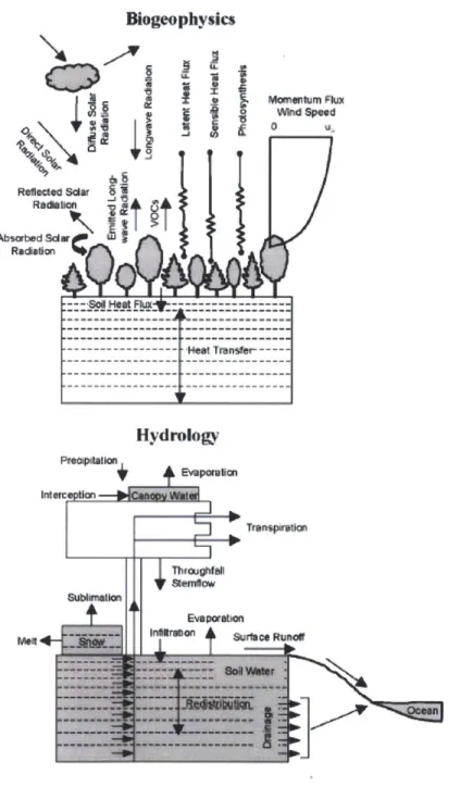
Figure 3-5: The biophysical and hydrological processes simulated in the Community Land Model (Oleson et al., 2004).

Figure 3-5 presents the biogeophysical and hydrological processes simulated in CLM

3.5. CLM-AG uses these same routines for crop columns to preserve consistency.

Evearetso