Global climate modeling of the Martian water cycle with improved microphysics and radiatively active water ice clouds

(1)

HAL Id: hal-01044402

https://hal.archives-ouvertes.fr/hal-01044402

Submitted on 12 Sep 2020

HAL is a multi-disciplinary open access

archive for the deposit and dissemination of

sci-entific research documents, whether they are

pub-lished or not. The documents may come from

teaching and research institutions in France or

abroad, or from public or private research centers.

L’archive ouverte pluridisciplinaire HAL, est

destinée au dépôt et à la diffusion de documents

scientifiques de niveau recherche, publiés ou non,

émanant des établissements d’enseignement et de

recherche français ou étrangers, des laboratoires

publics ou privés.

clouds

T. Navarro, J.-B. Madeleine, François Forget, A. Spiga, E. Millour, Franck

Montmessin, Anni Määttänen

To cite this version:

T. Navarro, J.-B. Madeleine, François Forget, A. Spiga, E. Millour, et al.. Global climate

mod-eling of the Martian water cycle with improved microphysics and radiatively active water ice

clouds. Journal of Geophysical Research. Planets, Wiley-Blackwell, 2014, 119 (7), pp.1479-1495.

�10.1002/2013JE004550�. �hal-01044402�

(2)

RESEARCH ARTICLE

10.1002/2013JE004550

Key Points:

• Radiatively active clouds impact atmospheric water vapor and ice in a GCM

• Cloud microphysics with dynamic nuclei is needed in GCMs

Correspondence to:

T. Navarro,

Thomas.Navarro@lmd.jussieu.fr

Citation:

Navarro, T., J.-B Madeleine, F. Forget, A. Spiga, E. Millour, F. Montmessin, and A. Määttänen (2014), Global cli-mate modeling of the Martian water cycle with improved microphysics and radiatively active water ice clouds,

J. Geophys. Res. Planets, 119, 1479–1495,

doi:10.1002/2013JE004550.

Received 2 OCT 2013 Accepted 7 JUN 2014

Accepted article online 13 JUN 2014 Published online 8 JUL 2014

Global climate modeling of the Martian water cycle

with improved microphysics and radiatively

active water ice clouds

T. Navarro1_{, J.-B Madeleine}1,2_{, F. Forget}1_{, A. Spiga}1_{, E. Millour}1_{, F. Montmessin}3_{, and A. Määttänen}3

1_{Laboratoire de Météorologie Dynamique, CNRS/UPMC/IPSL, Paris, France,}2_{Formerly at Department of Geological}

Sciences, Brown University, Providence, Rhode Island, USA,3_{Laboratoire Atmosphères, Milieux, Observations Spatiales,}

CNRS/UVSQ/IPSL, Guyancourt, France

Abstract

Water ice clouds play a key role in the radiative transfer of the Martian atmosphere, impacting its thermal structure, its circulation, and, in turn, the water cycle. Recent studies including the radiative effects of clouds in global climate models (GCMs) have found that the corresponding feedbacks amplify the model defaults. In particular, it prevents models with simple microphysics from reproducing even the basic characteristics of the water cycle. Within that context, we propose a new implementation of the water cycle in GCMs, including a detailed cloud microphysics taking into account nucleation on dust particles, ice particle growth, and scavenging of dust particles due to the condensation of ice. We implement these new methods in the Laboratoire de Météorologie Dynamique GCM and find satisfying agreement with the Thermal Emission Spectrometer observations of both water vapor and cloud opacities, with a significant improvement when compared to GCMs taking into account radiative effects of water ice clouds without this implementation. However, a lack of water vapor in the tropics after Ls = 180◦is persistent in simulations compared to observations, as a consequence of aphelion cloud radiative effects strengthening the Hadley cell. Our improvements also allow us to explore questions raised by recent observations of the Martian atmosphere. Supersaturation above the hygropause is predicted in line with Spectroscopy for Investigation of Characteristics of the Atmosphere of Mars observations. The model also suggests for the first time that the scavenging of dust by water ice clouds alone fails to fully account for the detached dust layers observed by the Mars Climate Sounder.

1. Introduction

The Martian water cycle is an important component of the Martian climate. The repeatable seasonal cycle of water vapor was first characterized from orbit by the Viking Mars Atmospheric Water Detector [Jakosky and Farmer, 1982] and later monitored for several years by the Thermal Emission Spectrometer (TES) onboard Mars Global Surveyor (MGS) [Smith et al., 2001; Smith, 2004], as well as the Mars Express instru-ments [Fedorova et al., 2006; Fouchet et al., 2007; Tschimmel et al., 2008; Maltagliati et al., 2011]. TES was also used to monitor the water ice cloud opacities around 2:00 P.M. local time. In light of these measurements, a first generation of numerical models that are able to simulate the main characteristics of the observed cycle was developed by introducing water vapor sublimation, condensation, and transport in three-dimensional global climate model (GCM). Richardson and Wilson [2002] first described the major mechanisms control-ling the cycle. Montmessin et al. [2004] obtained similar results and analyzed the importance of clouds in the overall water transport. However, these models did not take into account the radiative effect of water ice clouds which had long been assumed to be negligible [Zurek et al., 1992].

It is only recently that clouds have been acknowledged to play a key role on the temperature structure of the Martian atmosphere. Haberle et al. [1999], Colaprete et al. [1999], and Hinson and Wilson [2004] showed that they could create thermal inversions and explain temperature profiles observed in locations where clouds were present. Wilson et al. [2008] showed that the atmospheric temperatures in the equa-torial region could only be fully explained by taking into account the radiative effect of clouds. Finally, Madeleine et al. [2012] studied the local and global effects of radiatively active clouds in the Labora-toire de Météorologie Dynamique (LMD) GCM and showed that they help reduce global temperature biases between model and observations throughout northern spring and summer. This was also briefly discussed by Urata and Toon [2013] using a new GCM derived from the National Center for Atmospheric

(3)

Research Community Atmosphere Model. However, Madeleine et al. [2012], Urata and Toon [2013], and unpublished studies performed with other Martian climate models (NASA Ames GCM, [Haberle et al. 2011]; Geophysical Fluid Dynamic Laboratory (GFDL) GCM, R. J. Wilson, personal communication, 2014) found that, taking into account, the radiative effects of clouds had a strong negative impact on the modeled water cycle which cannot be simulated realistically. In most cases, it tended to be much drier than without radia-tive effects of clouds. Haberle et al. [2011] attributed this to unrealistic spurious water ice clouds that form above the northern polar cap during summer, affecting the global radiation budget at the surface, and therefore reducing the total amount of water vapor released in the atmosphere. Urata and Toon [2013] also found that “it was extremely difficult to simultaneously duplicate the observed cloud opacities in the high summer latitudes due to the highly coupled nature of the polar cap temperature, cloud formation, atmo-spheric heating and cooling by clouds, and the saturation vapor pressure.” They concluded that their model failed “to take into account some process that occurs at high latitudes in the summer hemisphere that sup-presses cloud formation,” and suggested that this process could be supersaturation. They were inspired by the observations of Maltagliati et al. [2011] who reported the presence of water vapor in supersaturation above the hygropause using Mars Express SPICAM (Spectroscopy for Investigation of Characteristics of the Atmosphere of Mars) solar occultation. In most GCMs, including the LMD GCM until today, such supersatura-tions were not taken into account. Condensation was assumed to occur when saturation is reached, and all the excess water converted into ice.

In this paper we investigate the eﬀects of radiatively active clouds on the atmospheric water ice and vapor in a GCM that consistently model the nucleation of cloud particles and their growth in supersaturated atmo-sphere. We show that it prevents the formation of water ice clouds above the northern polar cap during summer. A description of the new water cycle model (including the detailed microphysics scheme, as well as a better representation of permanent ice caps) is given in section 2. Section 3 describes the GCM results, the necessity for the microphysical modeling of clouds, and the inﬂuence of tunable parameters. Section 4 compares simulations to TES measurements and discusses the various interactions and features of the water cycle.

2. Model Description

The model used in this paper is the Mars general circulation model (GCM) developed at Laboratoire de Météorologie Dynamique (LMD) [Forget et al., 1999, 2011].

The dynamical core that integrates the fluid hydrodynamic equations for the atmosphere is a finite differ-ence numerical model. The horizontal discretization is a longitude-latitude grid, and the vertical discretiza-tion uses hydrid𝜎-pressure coordinates. Due to the longitude-latitude grid, the Courant-Friedrichs-Lewy criterion is violated in upper latitudes, and a classical Fourier filter is applied at the pole to the dynamical variables, such as the horizontal wind, the temperature, and the surface pressure [Forget et al., 1999]. The physical parametrization of the model takes into account emission and absorption of CO2gas in

infrared, as well as emission, absorption, and scattering of two aerosols: airborne dust [Madeleine et al., 2011] and water ice [Madeleine et al., 2012]. The seasonal variations of atmospheric mass by condensation of CO2

[Forget et al., 1998] reproduce the pressure cycle as measured by Viking lander [Hess et al., 1980]. A subgrid scale convection using a thermal plume model is parameterized in the planetary boundary layer [Cola¨ıtis et al., 2013]. A photochemical module with 15 species [Lefèvre et al., 2004, 2008] is implemented in the model and is used only in one speciﬁc case in section 4.3. The model has an extension to the thermosphere up to the exobase around 250 km [Angelats i Coll et al., 2005; González-Galindo et al., 2009], but it is not activated in the simulations of the present paper.

The ground is modeled with 18 subsurface layers down to 18 m with a horizontally and vertically varying thermal inertia to solve the thermal conduction for underground thermal inertia values ranging from 30 to 2000 J m−2_K−1_s−1∕2_{. The CO}

2cycle is tuned thanks to, among other things, the CO2ice albedo and the

underground thermal inertia in the model, representing the underground water ice centimeters below the surface from midlatitude to the pole in both hemispheres [Haberle et al., 2008].

Airborne dust distribution is simulated using a “semi-interactive” scheme [Madeleine et al., 2011]: the shape of the dust vertical proﬁles freely evolves with atmospheric mixing, but the total column values are rescaled to match the observed opacities as compiled by Montabone et al. [2014]. The transported dust is modeled using a two-moment scheme [Madeleine et al., 2011]. The two moments are the number mixing ratio dust

(4)

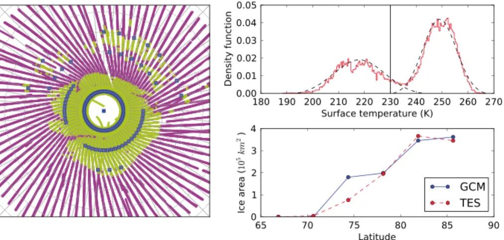
Figure 1. Surface temperatures betweenLs = 90◦andLs = 120◦for latitudes above 65◦N and at local times between 10:00 A.M. and 5:00 P.M. Geographic distribution of daytime temperatures from TES betweenLs = 110◦andLs = 115◦ above 65◦N colder than 230 K (beige) and warmer (pink), and (left) representation in the GCM. (right, top) Distribution of these temperatures (red) and two Gaussian ﬁts (dashed) of the underlying cold and warm distributions. (right, bottom) Ice as a function of latitude from TES temperatures and as prescribed in the GCM.

particles (number of particles per kilogram of air) and the mass mixing ratio (kilogram per kilogram of air). Each quantity is advected independently and, assuming a lognormal size distribution, the eﬀective radius of dust particles can be computed. A constant and homogeneous dust-lifting value is used as a source of dust, balanced by a size-dependent gravitational sedimentation. Below we describe how this scheme is now used to parameterize the scavenging of dust particles by water ice condensation.

2.1. Ground Water Ice

2.1.1. Permanent Ice Reservoirs

The model uses thermal inertia and albedo derived from TES measurements [Putzig and Mellon, 2007]. However, the permanent water ice reservoirs on the northern polar ice cap, the main source of Martian atmospheric water in the model, are modeled with their own prescribed albedo and thermal inertia, instead of using surface values derived from spacecraft data. Using true ice thermal inertia and albedo data is indeed more suitable to a GCM, as it simulates actual perennial surface water ice, instead of relying on measurements that mix bare ground and ice within a GCM grid mesh.

Albedo and thermal inertia values of this ice are left as tunable parameters because one cannot exactly know the ice surface purity, although acceptable values range from 0.3 to 0.5 for albedo [Wilson et al., 2007] and 500 to 2000 J m−2_K−1_s−1∕2_{[Putzig and Mellon, 2007] for thermal inertia.}

The extent of a permanent ice reservoir in the GCM is simply the area of the corresponding mesh deﬁned by the longitudinal-latitudinal grid. One of the main parameters for water vapor release is the surface tem-perature controlled by direct solar illumination or, equivalently, the latitude of the permanent ice reservoir, which can be used to deﬁne permanent reservoirs.

2.1.2. Amount of Permanent Ice

A new representation of perennial surface ice is used to better constrain the water cycle than the simple dis-tributions usually used in GCMs [Richardson and Wilson, 2002; Montmessin et al., 2004]. The actual locations occupied by perennial surface water ice can be derived from summertime TES surface temperature because water ice tends to remain signiﬁcantly colder than bare ground during northern summer as illustrated on Figure 1 (right, top). In practice, we assumed that permanent ice is present when surface temperatures remain below 230 K above 65◦N between Ls = 90◦and Ls = 120◦, and that the corresponding GCM grid points would be covered by water ice. This results in a realistic spatial distribution of permanent ice in the GCM with a good approximation of the ice variation with latitude. Figure 1 (right, bottom) compares the total area of ice at a given latitude in the GCM (in the resolution used in this paper) and as retrieved from the observations (corrected to account for the imperfect spatial coverage). The modeled ice coverage is in good agreement with the observations, except at latitude 75◦N, where the ice is overestimated in the GCM. However, as explained in section 4.5, this overestimation does not result in an overestimation of water vapor release.

(5)

2.1.3. Seasonal Frost

As for polar ice reservoirs, seasonal frost can modify surface albedo. We use a threshold value of 5 μm, as in Richardson and Wilson [2002] and Montmessin et al. [2004], of surface ice deposition to change surface albedo from bare soil albedo to the same value prescribed for the perennial north polar cap reservoirs. This choice was made in order to reduce the number of tunable parameters. In reality, both albedos are sig-niﬁcantly variable in space and time (in the future it may be possible to improve—and complicate—the model by better representing the perennial surface ice and the frost albedo). The maximal extent of the observed seasonal frost to latitudes around 50◦N and 50◦S is reproduced. The diﬀusion of water vapor into the regolith is not included.

2.1.4. Sublimation Scheme

The sublimation of surface ice deposits is controlled by the surface turbulent ﬂux [Forget et al., 1999; Montmessin et al., 2004]:

Ew=𝜌Cdu∗(qsat− qw) (1)

where E_wis the turbulent flux of water into the lowest atmospheric model layer,𝜌 is the atmospheric density near the ground, C_dis the aerodynamic drag coefficient, u_∗is the friction velocity, and q_wis the mass mixing ratio of water vapor (q_satis the saturation mass mixing ratio at the surface temperature) in the first layer. C_d depends, among other variables, on the surface roughness coefficient and on the Richardson number [see Cola¨ıtis et al., 2013]. Equation (1) shows that the amount of water ice that is sublimated depends on both the humidity and the intensity of the turbulent mixing close to the surface.

2.2. Microphysics

2.2.1. Cloud Microphysics Under Martian Conditions

In the previous studies performed with the GCM [Montmessin et al., 2004; Madeleine et al., 2012], the cloud scheme was rather simplistic: water vapor is turned instantaneously into ice, or the other way around, to reach the saturation pressure; and the number of ice particles is defined as a fixed fraction of available dust particles. However, it is well known that in the atmosphere the water vapor phase does not suddenly turn into a condensed phase as soon as saturation, mainly controlled by temperature, is reached. Instead, ice particles nucleate and grow onto airborne dust [see e.g., Määttänen et al., 2005]. Such processes have a tight control of the properties of the clouds as well as on the remaining vapor phase. Nucleation eventu-ally determines the number of dust nuclei onto which water vapor will condense. Inclusion of these two processes makes predictions for cloud particle size physically consistent and also allows the existence of substantial amounts of supersaturation (e.g., when dust nuclei are too sparse). We included a microphysics scheme adapted from Montmessin et al. [2002] in the GCM. The main motivations are to address the effect of dust scavenging by water ice clouds, allow supersaturation of water vapor, and correctly predict water ice clouds characteristics.

2.2.2. Nucleation

As on Earth, airborne dust is expected to play the role of condensation nuclei under Martian atmospheric conditions [Gooding, 1986], referred to below as CCN for Cloud Condensation Nuclei. Therefore, we assume that nucleation occurs within the frame of the theory of heterogeneous nucleation. As described in Montmessin et al. [2002], the number of activated CCN by nucleation depends on a poorly constrained con-tact parameter, m, given by m = cos𝜃 with 𝜃 the “contact angle” (in the liquid phase it is the angle of the interface between the droplet and its nucleus). In the case of a nucleation as efficient as possible, the contact would be maximized with m equal to 1. In reality, this contact parameter depends on the intrinsic properties of water and Martian dust. Laboratory experiments on Mars dust analogs have typically found values ranging between 0.97 and 0.93, or even lower values (down to m = 0.84) at temperatures below 180 K, with nucleation becoming more difficult when lowering temperatures [Trainer et al., 2009; Iraci et al., 2010; Phebus et al., 2011]. The sensitivity of the modeled water cycle with m is discussed in section 3.1. In practice, in the GCM, the dust particles which are activated are transferred into a new kind of tracer, the CCN. The quantity and size distribution of CCN is described in each model box by its own mass-mixing ratio and number-mixing ratio assuming a lognormal distribution and an effective variance of 0.1 (in other words, we use the two-moment scheme of Madeleine et al. [2011] for the dry dust particles, and add the CCN size distribution that differs from the dust size distribution). To implement the nucleation process itself (i.e., to compute the mass and the number of dust particles which become CCN at every time step in a model grid-box), we first discretize the dust distribution around the mean radius. Then, in each radius bin, we perform

(6)

nucleation as described in section 2.1 in Montmessin et al. [2002]. The new distributions of dust and CCN are the sum over the radius bins for the mass and the number of particles. We use five bins for this discretization from 0.1 to 50 μm. Tests did not show a significant difference when using 50 bins.

2.2.3. Condensation

We use the formulation of Montmessin et al. [2002] for the growth of ice crystals:

dr dt = 1 r ( S − S∗ Rc+ Rd ) (2)

with r the radius of the crystal (assumed to be spherical), S the saturation ratio between water vapor partial pressure and the saturation pressure, S∗_{the saturation ratio at equilibrium taking into account the crystal}

surface curvature (Kelvin eﬀect) and Rcand Rdthe heat and diﬀusive resistances described in Montmessin et

al. [2004, 2002].

We initially introduced equation (2) and the formulation for nucleation of Montmessin et al. [2002] in the GCM using a 15 min time step with an explicit numerical scheme. This led to a severe underestimation of rfor ice clouds formed in the model and an overestimation of the amount of CCN involved. Underestimat-ing the radius has dramatic eﬀects on the cloud evolution in case of radiatively active clouds. Indeed, if the same amount of ice is condensed on a greater number of particles, the resulting cloud has smaller particles and hence higher opacity. In particular, any local drop in temperature due to the radiative eﬀect of clouds is overestimated, leading to increased saturation ratio (even if the amount of water vapor decreases), rein-forcing nuclei activation. This positive feedback loop between cloud formation and temperature, controlled by the ice particles size and number, yields unrealistic cloud opacities. Again, radiatively active clouds mod-ify not only Martian dynamics on a large scale [Hinson and Wilson, 2004; Madeleine et al., 2012] but also the structure and the formation of the clouds themselves due to microphysical processes on the local scale. Therefore, it appears that the use of an elaborate microphysical scheme in a GCM needs to be followed by a careful understanding of the ice particle size dependence on the integration time step. Various tests with single-column model and 3-D simulations led us to conclude that it is necessary to couple both nucleation and condensation through subtimesteps no larger than 1 min. In particular, this was necessary to prevent the formation of unrealistic clouds above the North Pole during summer, as explained in section 3.3.

2.2.4. Scavenging

Scavenging is a key physical process on the Earth, allowing for the “cleaning” of the atmosphere from aerosols through water precipitation. On Mars, scavenging is thought to play a role in the dust cycle [Clancy et al., 1996], but detailed studies are lacking. Modeling scavenging of dust particles working as cloud nuclei is straightforward in our new cloud microphysical scheme as implemented: CCN are advected like any other tracer in the GCM. As nucleation occurs, dust particles are converted to CCN, incorporated into ice crys-tals, while the number of remaining “ice-free” dust particles is reduced accordingly. CCN sediment and the ice particles are released only after all of the ice crystals have sublimated, returning to the “ice-free” dust inventory.

In our model, one speciﬁcity is that the mass and number of dust particles are multiplied by a conversion factor at each time step so that the dust column matches the observed column opacities [see Madeleine et al., 2011]. We use the same conversion factor for CCN when it comes to getting actual values of mass and number at each time step. This implies the following two assumptions:

1. CCN do not aﬀect radiative transfer. In other words, dust captive into ice crystals does not interact with light and extinction by ice dominates.

2. The typical lifetime of CCN in ice particles is lower than the typical time associated with major dust changes. Indeed the conversion factor used for dust varies with time and space according to changes in prescribed dust opacity. If a dust particle is sequestered in an ice crystal, the conversion factor is then based on the local dust conditions and not on the conditions where and when the dust particle was captured by ice.

Within and below the clouds, the scavenging of dust by falling crystals which could intercept and coalesce with the dust particles is neglected. The mass ﬂux associated with this process can be estimated following Seinfeld [1986]. On Mars, it is 2 to 3 orders of magnitude smaller than the sedimentation ﬂux of CCN.

(7)

Table 1. Parameters Used for the Reference Run

Parameter Value

Contact parameterm 0.95

Eﬀective variance for sedimentation𝜈_eﬀ 0.1 Albedo of frost and permanent ice 0.35 Thermal inertia of permanent ice 800 tiu

3. Global Water Cycle Sensitivity

to Model Parameters

3.1. Parameters

Modeling the water cycle requires the setting of val-ues for four poorly constrained model parameters: the albedo of surface ice and frost, the thermal inertia of perennial water ice deposits, the contact parameter m, and the variance of the size distribution of the ice cloud particles which affects the radiative properties of the clouds and the sedimentation flux of ice cloud particles. This last point has a strong impact on the model results because the cloud particle size effective variance𝜈_effis directly used to calculate the sedimentation flux via an “effective” fall radius rsed _{= r}

c(1 +𝜈eﬀ)3used in the Stokes-Cunningham relationship for falling

particles [Montmessin et al., 2004], with rcthe mass mean radius This reﬂects the fact that, when it comes to

the mass transport of a population of particles due to sedimentation, rcis biased toward larger particles.

The three reference diagnostics, collected from observations, for the tuning values of the four model param-eters are (1) the sublimation peak of water vapor during northern summer solstice of 60 pr μm, (2) the zonal mean of the amount of atmospheric water vapor in the tropics during northern fall of 10 pr μm, and (3) the mean aphelion cloud belt opacity of 0.15 at 825 cm−1_{at a local time of 2 P.M. These diagnostics have}

been chosen because they refer to quantities that are handy for physical interpretation and they well con-strain the simulated water cycle. The sublimation peak controls most of the total atmospheric water vapor throughout the year on the whole planet, the opacity of the aphelion cloud belt constrains the impact of clouds on atmospheric temperatures [Madeleine et al., 2012], and the tropical water vapor is a good indicator of meridional transport of vapor from northern polar regions.

3.2. Reference Run

The results in this section are obtained by running the LMD GCM at a resolution of 64 × 48 on the longitude-latitude grid and 29 levels reaching a maximum altitude above ground of 0.02 Pa, about 80 km. The column dust opacity is prescribed at a given location and time using a scenario derived from observa-tional data [Montabone et al., 2014]. The scenario for Martian Year (MY) 26 has been used by default, because it is representative of years without a global dust storm. Results for other years are addressed in section 3.3. The tunable parameters have been set to the values compiled in Table 1. These speciﬁc values were chosen in order to obtain a realistic water cycle. The overall simulated water cycle is compared to TES observations [Smith, 2004] during MY26.

An equilibrated state for the water cycle is reached after 20 years of simulation (Figure 2). The main dif-ference between the modeled zonal average water vapor ﬁelds and the TES observations is the summer sublimation peak at the North Pole, whose amplitude is 30% too large, and the amount of water vapor in the Northern Hemisphere tropics after Ls = 180◦, which is too low in the GCM. The diﬀerence in timing for the peak of the frost sublimation in the Southern Hemisphere is mainly controlled by the seasonal timing of the CO2ice cap sublimation.

3.3. Global Eﬀect of the Improved Microphysics

The effect of the microphysics on the water cycle of the reference run is fundamental. This is illustrated in Figure 3 for two different simulations. The first one is the reference run, and the second one is the same simulation, except that the cloud microphysics scheme is not used and supersaturated water vapor is turned instantaneously into ice with a predefined number of ice particles, as in Montmessin et al. [2004]. The cloud opacity shows that, for this second simulation, the polar hood clouds persist throughout the sum-mer. As mentioned above, this situation is not realistic, as observations by the MGS Mars Orbiter Camera [Wang and Ingersoll, 2002] and TES [Smith et al., 2002] show that clouds above the Northern polar cap dur-ing summer are intermittent, scattered across the polar region, and very faint. For the reference run, we see a quasi-absence of polar clouds between Ls = 100◦and Ls = 145◦, as expected from observations. When comparing the two simulations, the infrared downward radiative flux is greater with the simulation without microphysics, while the visible flux is smaller. This is simply due to the fact that clouds limit the vis-ible sunlight that reach the surface and they emit in the infrared band. The total downward radiative flux to the surface is substantially smaller for the simulation without microphysics, except at local time 2 A.M. after Ls = 120◦. This explains why the surface of perennial surface ice is colder for the simulation without microphysics, at all local times during the whole summer.

(8)

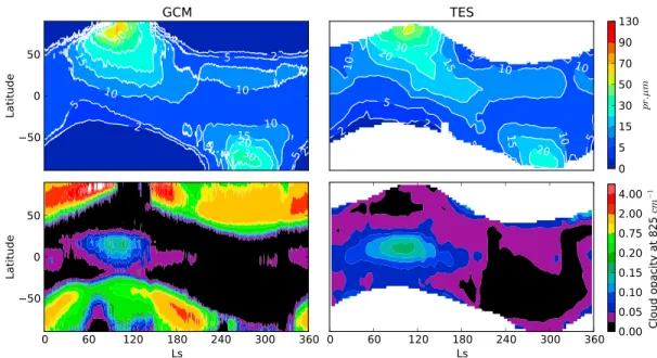
Figure 2. Zonal mean quantities at 2 P.M. local time for MY26 of atmospheric water vapor as simulated by the (top left)

GCM and observed by (top right) TES, (bottom left) GCM cloud opacity and (bottom right) TES cloud opacity.

As a consequence, the surface ice is sublimated in smaller quantities in the simulation without microphysics. Therefore, the column-integrated water vapor in the atmosphere is subsequently decreased for the simula-tion without microphysics. When the polar clouds reappear after Ls = 145◦in the reference simulation, there is a decrease of the atmospheric water vapor because it is trapped in the clouds. Polar clouds also increase the total 2 A.M. radiative ﬂux and the surface temperature after Ls = 145◦, but the surface ice sublimation is not enhanced enough to overcompensate for the loss of water vapor.

In this example, the continuous presence of polar clouds in the simulation without microphysics causes a decrease of the amount of water vapor released in the atmosphere, as in Haberle et al. [2011], Madeleine et al. [2012], and in the GFDL GCM (R. J. Wilson, personal communication). This behavior is very dependent on the properties of clouds simulated in the model and could also enhance the amount of water vapor if the total flux happens to be increased when compared to the reference simulation, if the infrared radiative flux to the surface caused by clouds overcompensates the loss of visible flux. The only realistic way to prevent such feedback loops is by having clear sky conditions during the summer thanks to the use of the microphysics, such as illustrated by the reference simulation.

One should also be aware that the simulation without microphysics induces a global water cycle that is not in a steady state, and the next years of simulation would have less and less water vapor at the pole and on the whole planet.

It is worth noting that even in the reference simulation, polar clouds that exist before Ls = 100◦seem to still play a role on the surface temperature and the amount of atmospheric water vapor. There is an extreme sensitivity of the whole water cycle to the critical short period of the summer solstice at the North Pole as already noted by Urata and Toon [2013].

3.4. Sensitivity to Parameters

3.4.1. Surface Ice Albedo and Thermal Inertia

The reference simulation is a basis for analysis and comprehension of the water cycle and of the sensitiv-ity to the previously mentioned parameters. Figures 4, 5, 6, and 7 explore the inﬂuence of parameters on the atmospheric water vapor and clouds after 5 years of simulation starting from the same reference steady state of the reference run. A decrease of albedo or thermal inertia of the perennial surface ice increases the overall humidity and cloud opacity, especially in the aphelion cloud belt (Figures 4 and 5). With such param-eters, quantities sublimated at the North Pole are larger than in the reference run due to warmer surface temperatures for the perennial surface ice. Because of this, the period during which the North Pole is free of clouds is reduced in these warm and wet cases, thus giving more weight to the undesired relation between clouds and the total water vapor released in the atmosphere, as explained in section 3.3. The use of a smaller

(9)

Figure 3. Zonal mean quantities for latitudes 75◦N to 90◦N for simulations with microphysics (plain) and without (dashed), betweenLs = 60◦andLs = 160◦. Values (left column) at local time 2 P.M. and (right column) at local time 2 A.M. (first row) The cloud opacity at 825 cm−1_{. (second row) The total radiative flux received at the surface (black), and} its infrared (red) and visible (blue) contributions. (third row) The surface temperatures for the perennial surface ice only. (fourth row) The atmospheric water vapor. Note that the vertical axis is not the same for the radiative flux budget at the two different local hours, unlike in the other rows.

time step for microphysics does not change the resulting cloud ﬁelds in simulations. Thus, it remains unclear if this behavior would be real in cases with higher surface temperatures or is a limitation of the model for these cases.

Changing values of the ice thermal inertia or albedo has the same qualitative impact on the sublimation peak at the North Pole, although the impact of each parameter on the diurnal cycle of surface temperatures of surface perennial ice is diﬀerent. A decrease of albedo or thermal inertia results in higher water vapor col-umn values from Ls = 250◦to Ls = 360◦in the Northern Hemisphere. However, the higher sublimation peak near the South Pole is more emphasized with the decrease of albedo than with the decrease of ther-mal inertia. This can be explained by the fact that therther-mal inertia only impacts the perennial surface ice on the North Pole, whereas albedo impacts any surface ice thicker than 5 μm. Hence, seasonal frost sublima-tion is enhanced in those two places when the ice albedo is decreased. Conversely, an increase of albedo or thermal inertia tends to dry out the water cycle and produce fainter aphelion clouds.

3.4.2. Nucleation Contact Parameter and Eﬀective Variance of the Cloud Particle Size Distribution

The contact parameter controls the amount of activated nuclei in water ice clouds. Increasing the contact parameter, i.e., the eﬃciency of nucleation, increases the number of ice particles for a given cloud mass (as long as all CCN are not activated). Hence, the size of ice particles is lowered and the sedimentation of

(10)

Figure 4. GCM zonal mean quantities during daytime for MY26 of (top row) atmospheric water vapor and (bottom row) cloud opacity with three diﬀerent values

of albedo for perennial surface ice: (left) 0.3, (middle) 0.35, and (right) 0.4.

clouds is less effective. This impacts the transport of water from polar regions to lower latitude regions, which is made easier due to longer lasting clouds [Montmessin et al., 2004]. It follows that the atmosphere keeps more water vapor (Figure 6). The same statement stands for the effective variance of sedimentation (Figure 7): a decrease of the variance decreases sedimentation and increases the global amount of water vapor in the atmosphere. Varying the contact parameter between 0.94 and 0.96 as presented here changes the number of ice particles by 2 orders of magnitude. This helps to prevent the formation of polar clouds above the North Pole around summer solstice, more efficiently than what a change of the effective variance for sedimentation would produce. This is shown in Figure 6 (left), where the sublimation peak at the North Pole is less pronounced than the three other wet cases for the other parameters. In other words, increas-ing the contact parameter tends to increase the water vapor column in the tropics rather than the vapor near the North Pole. Conversely, an increase of sedimentation due to a smaller contact parameter or a larger effective variance limits the transport of water and tends to dry the atmosphere.

(11)

of contact parameter: (left) 0.94, (middle) 0.95, and (right) 0.96.

4. Analysis and Comparison With Observations

4.1. Eﬀect of Radiatively Active Clouds on the Global Water Cycle

One simple and obvious way to assess the effect of radiatively active clouds on the modeled global water cycle is to compare simulations with and without radiatively active clouds. All other things being equal, the main difference is the amount of vapor sublimated at the North Pole that is almost twice lower with radia-tively inactive clouds than with active clouds (not shown). This discrepancy is caused both by the direct effect of radiatively active clouds on the surface temperature before Ls = 90◦and the induced stronger baroclinic wave activity at the same period that generates stronger winds and enhances sublimation flux from surface to atmosphere, as can be inferred from section 2.1.4. The global amount of water vapor is pri-marily controlled by this sublimation peak at the North Pole. To explore factors other than this dominant one, we lowered the surface ice albedo and thermal inertia in the simulation with radiatively inactive clouds to increase the surface temperature and thus the sublimating flux of vapor. The most prominent difference between a simulation with radiatively active clouds and one without is then the amount of atmospheric water vapor that is advected from the North Pole to the tropics during northern spring and summer, as seen

of cloud particle size distribution eﬀective variance for sedimentation: (left) 0.01, (middle) 0.1, and (right) 0.2. Note that we keep the value of the eﬀective variance for the radiative transfer to the same value of 0.1 in all cases.

(12)

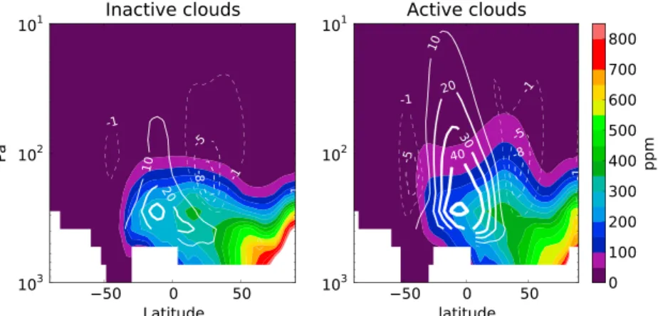
Figure 8. Zonal mean of atmospheric water vapor (colors, volume mixing ratio) and stream function (108kg/s, contoured lines) averaged overLs = 120◦–150◦(right) with radiatively active clouds and (left) without.

in Figure 8. This is due to the strengthening of the Hadley cell with radiatively active clouds [Madeleine et al., 2012] which traps more eﬃciently water vapor at latitudes 40◦to 60◦N. Indeed, the vertical extension of the Hadley cell above the hygropause is more emphasized with radiatively active clouds than without. This manifestation of the so-called “Clancy eﬀect” Clancy et al. [1996] is reinforced by radiatively active clouds and changes the equatorward transport of water vapor.

4.2. Eﬀect on Dust Vertical Distribution

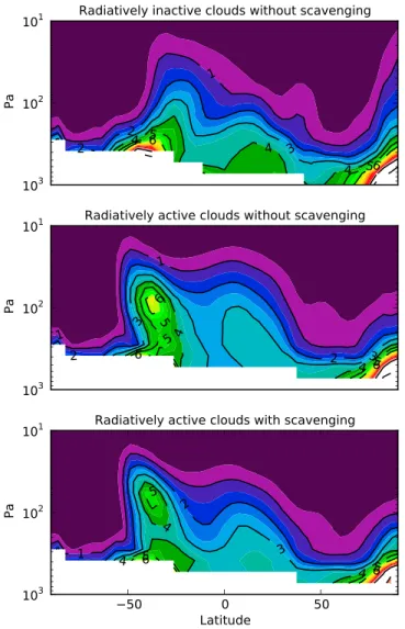
One motivation for the inclusion of dust scavenging by water ice clouds was to assess its influence on dust vertical distribution. In particular, it has been suggested that scavenging could explain the formation of the detached dust layers observed by Mars Climate Sounder [McCleese et al., 2010; Heavens et al., 2011a] by the enrichment of dust below the ice clouds (by releasing the dust when the cloud sublimates) or by depletion in the clouds (by decrease of dust quantities due to nucleation within the cloud). It is possible to assess the effect of scavenging on the whole simulation and especially on the dust distribution by simply turning off the interactions of clouds with airborne dust in the simulations. In other words, if a cloud forms, CCN are acti-vated but no dust is removed from the ambient atmosphere. When ice particles sublimate, the released CCN just disappear and are not turned back into dust. From the reference simulation, it appears that turning on and off scavenging does not help to produce more dust-detached layers. However, even without scaveng-ing, the radiative effect of clouds sometimes favors the formation of such layers, as illustrated in the example of Figure 9. This is due to the reinforcement of semidiurnal waves with radiatively active clouds [Hinson and Wilson, 2004] that locally enhance upward winds. However, such layers only occur at rare and specific loca-tions in our simulaloca-tions. The example given in Figure 9 is the most evident one with a detached layer and is not representative of the dust vertical distribution throughout the simulation. Therefore, radiatively active clouds alone cannot account for the formation of detached layers of dust, but it is worth noting their possi-ble contribution in combination with other possipossi-ble mechanisms [Spiga et al., 2013; Rafkin, 2012; Heavens et al., 2011b].

4.3. Supersaturation

The use of our new microphysical scheme for the formation of water ice clouds opens the possibility to simulate supersaturation.

Above the hygropause, the lack of dust particles to trigger nucleation allows water vapor to remain in a supersaturated state. In that case, the most prominent process that affects water vapor is the photodissocia-tion of water vapor. Because of the exponential relaphotodissocia-tion of saturaphotodissocia-tion with temperature, a few ppm of water vapor can correspond to a huge saturation ratio, and photodissociation cannot be neglected. Therefore, we used the photochemistry module implemented in the GCM [Lefèvre et al., 2004] to study the supersatura-tion of water vapor in dedicated simulasupersatura-tions. The model is vertically extended when using this module to take into account all photochemical processes that take place at different altitudes. The use of the photo-chemistry module and this vertical extension does not significantly change the simulated water cycle, as quantities of supersaturated water vapor affected by the photochemistry are very small when compared to

(13)

Figure 9. Mass-mixing ratio of airborne dust (ppm) at longitude 25◦W during the periodLs = 90◦–120◦for a GCM simulation (top) with-out radiatively active clouds, (middle) with radiatively active clouds but without scavenging, (bottom) with both radiatively active clouds and scavenging.

the typical amount of water vapor (less than 2 ppm versus hundreds of ppm). The photochemistry mod-ule and this extension were not used for previous simulations, as it is computationally expensive.

Figure 10 shows supersaturation profiles from the GCM, at the same locations as those reported from SPI-CAM solar occultation measurements in Maltagliati et al. [2011]. When com-pared to Figure 3 of Maltagliati et al. [2011], the Northern Hemisphere values are in agreement with the obser-vations, with a typical saturation ratio, S, of at most 10 between 30 and 50 km before Ls = 90◦and between 40 and 60 km after. In the Southern Hemi-sphere, some profiles after Ls = 75◦ match the observations but about 10 km higher than observed. More-over, there is a clear discrepancy before Ls = 75◦with peaks at S = 100 between 20 and 40 km, and S> 1000 above 60 km. This can be explained by the vicinity of those profiles to the strong temperature gradient of the polar night.

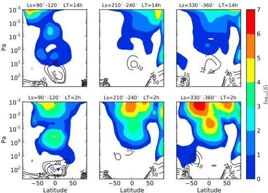
Figure 11 shows the structure of super-saturation up to 0.001 Pa at three diﬀerent seasons, as predicted by the GCM. Supersaturated water vapor remains above the water ice clouds. The pattern of supersaturation varies signiﬁcantly with local time, mainly

(14)

Figure 11. Base-10 logarithm of water vapor saturation ratio (shaded) and water ice volume mixing ratio in ppm at local

times (top row) 2 P.M. and (bottom row) 2 A.M., averaged over (left)Ls = 90◦–120◦, (middle)Ls = 210◦–240◦, and (right) Ls = 330◦–360◦.

because of the diurnal cycle of temperature. At Ls = 210◦–240◦and Ls = 330◦–360◦, temperature clearly controls the boundary of supersaturated water vapor.

The GCM fails to form dust-detached layers and might also miss the actual distribution of dust above the hygropause [Heavens et al., 2011a; Määttänen et al., 2013] that coexists with supersaturated water vapor [Maltagliati et al., 2013]. Therefore, we can wonder whether a supersaturated ratio above 103_{is realistic or}

not. It reaches the limits of our knowledge of dust distribution at these altitudes. Even without the pres-ence of dust, homogeneous nucleation (the formation of ice without another support) could be taken into account for such saturation ratios, which is not the case in the present model and is signiﬁcant for a ratio S > 105_{at 50 km [Määttänen et al., 2005]. All in all, such considerations do not aﬀect the total amount}

of atmospheric water in simulations because this supersaturated water vapor corresponds to negligible amounts of water vapor, less than one ppm.

4.4. Polar Ground Ice Budget

The improved representation of permanent surface ice on the North Pole gives insights into the fate of polar ice. Figure 12 shows that the long-term stability of permanent ice depends on the latitude of the con-sidered deposit. Ice is accumulating on the central cap at latitudes above 80◦N, whereas ice outliers are being hollowed at a rate of 1 mm/yr. Conversely, in southern polar regions, ice is accumulating at a rate of 0.5 mm/yr (not illustrated). This instability of surface ice that does not signiﬁcantly vary on a few years timescale and therefore supposed as perennial in atmospheric models, could be of great interest for recent climate changes and paleoclimatology. However, given the current uncertainties and limitations of the model to represent the water cycle, this question requires further investigation and is out of the scope of the present paper. The current version of the GCM suggests that the water ice reservoirs are not in an annual equilibrium state.

4.5. Exploration of Parameter Space and Tuning of the Water Cycle

The issue about the dry tropics raised in section 3.2 and explained in section 4.1 motivates a change of the values of these model parameters toward wetter simulations. A change of albedo, thermal inertia, or eﬀec-tive variance would indeed increase the water vapor in the tropics, but the maximum of water vapor at the North Pole would also be increased as seen in section 3.4, in stark contrast with observations.

(15)

Figure 12. Annual budget of permanent surface ice atLs = 0◦for the perennial surface ice on North Pole as defined in the GCM in mm/yr. White indicates this mesh grid is not defined as a permanent ice reser-voir in the GCM. Positive values indicate an increase of ice. A contour of albedo derived from TES observations is shown to indicate the distribution of ice on a finer scale.

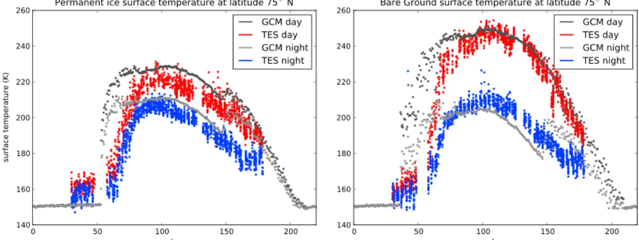
Furthermore, a decrease of albedo or thermal inertia would result in greater surface temperatures than in the refer-ence simulation. However, this would not be realistic because modeled temperatures are already slightly too high compared to the observations, as shown in Figure 13. One can see that the values of albedo and thermal inertia selected for the reference run yields temperatures 5 K warmer on the average than observed for permanent surface ice.

Another possibility would be to change the distribution of perennial surface water ice, described in section 2.1.2. The extent of this distribution, shown in Figure 1, directly controls the amount of water vapor released by surface sub-limation in polar regions. However, as mentioned in section 2.1.2 the amount of perennial surface ice is already slightly greater in the GCM at latitude 75◦N than in the surface ice distribution retrieved from TES tempera-ture observations (see Figure 1, right, bottom). Thus, further increasing the coverage of perennial surface ice would not be realistic.

An attractive option would be to increase the value of the contact parameter m to increase the amount of water vapor in the tropics. Figure 14 shows that increasing the value of the contact parameter helps to match the quantities of water vapor at the equator past Ls = 180◦. However, the maximum of water vapor around Ls = 180◦is then less well represented. The increase of water vapor in northern latitudes between Ls = 120◦and Ls = 180◦is controlled by the advection of water vapor sublimated at the North Pole, whereas the decrease after Ls = 180◦is controlled by the sedimentation flux of ice particles in the tropics. Increasing maffects the size of particles and therefore modifies the water vapor decrease after Ls = 180◦. It has no effect on the lack of southward vapor advection due to a stronger Hadley cell. A representation of the water vapor closer to observations at equator could only be obtained without radiatively active clouds, which yields a correct maximum at 15 pr μm at Ls = 180◦, even though the maximum is well represented at 40◦N at Ls = 120◦for the three cases (inactive clouds, active clouds with m = 0.95, and m = 0.96).

(16)

Figure 14. Zonal mean quantities during daytime for MY26 of

atmo-spheric water vapor at (top) latitude 40◦N and (bottom) equator of TES (grey) and GCM for three diﬀerent runs: reference run (blue), same as reference run but with contact anglem = 0_.96(red) and same as ref-erence run but without radiatively active clouds and diﬀerent tuning (see text) (green).

This raises the question of the improve-ment of the water cycle with the current version of the GCM. Even if it is possible to assess the local effect of each parameter, the complete simula-tion is a complex balance after at least a decade of integrations before reach-ing a steady state, and the best way to quantitatively assess the global impact of one single parameter is through an empirical approach. In such a sys-tem, effects of parameters are coupled and no better set of parameters than the one used for the reference run has been found. Given the current GCM configuration, we cannot find any sig-nificant leverage on the strength of the Hadley cell after summer solstice without degrading the water cycle.

5. Conclusion

We have included a new microphysi-cal scheme in a global climate model that takes into account the radiative eﬀects of clouds to represent cloud particles nucleation on dust particles, ice particle growth, and scavenging of dust particles resulting from the condensation of ice. The use of this microphysical scheme prevents the formation of clouds above the poles around summer solstice that occurs when microphysics is not well taken into account, and which has been found to negatively alter the model-ing of the water cycle in many Martian GCMs takmodel-ing into account the radiative eﬀect of clouds [Madeleine et al., 2012; Urata and Toon, 2013; Haberle et al., 2011, and R. J. Wilson, personal communication]. This enables a more realistic representation of the water cycle with radiatively active clouds. For this purpose, we have explored the model sensitivity to model parameters not well known from observations in order to tune the water cycle to match available observations and in particular TES data.

This study leads us to conclude that the radiative effects of clouds are (at least) twofold: First, there is an impact on the cloud formation itself, due to the local change in atmospheric temperature that generates a feedback on the cloud formation. Handling the cloud formation with such radiative effects is critical for the simulation of the Martian water cycle with a GCM. Second, there is an impact on the Hadley circulation that is reinforced in comparison with simulations without radiative effects of clouds. This changes the equator-ward transport of water, leading to a dry bias in tropics when compared to observations. The exploration of the influence of the four physical parameters on the water cycle leads us to conclude that this dry bias cannot be completely corrected with the current representation of the water cycle in the GCM. Neverthe-less, overall, the new model is more consistent with observations than before, thanks to a simulated thermal structure that is more consistent with observations because of the use of radiatively active clouds which leads to a qualitative improvement of the modeled water cycle. The coupling between atmospheric temper-atures and the water cycle, through clouds and global circulation, is so strong that the modeling of these two coupled quantities should be seen as an inseparable whole.

This new representation also allows the exploration of new topics, such as vapor supersaturation in the Mar-tian atmosphere, the long-term stability of perennial surface ice, and the question of missing sources and sinks in the water cycle. It has also been found that dust scavenging by water ice clouds is most probably not the cause of dust-detached layers observed in the Martian atmosphere, even though atmospheric waves enhanced by the radiative eﬀect of clouds sometimes help the formation of detached layers. The inclu-sion of new physical processes allowed us to point out model sensitivities that should be addressed before

(17)

adapting any GCM to paleoclimates, with warmer and wetter conditions than today and for which radiative eﬀects of clouds have long been neglected in GCM studies.

References

Angelats i Coll, M., F. Forget, M. A. López-Valverde, and F. González-Galindo (2005), The ﬁrst Mars thermospheric general circulation model: The Martian atmosphere from the ground to 240 km, Geophys. Res. Lett., 32, L04201, doi:10.1029/2004GL021368. Clancy, R., A. W. Grossman, M. J. Wolﬀ, P. B. James, D. J. Rudy, Y. N. Billawala, B. J. Sandor, S. W. Lee, and D. O. Muhleman (1996), Water

vapor saturation at low altitudes around Mars aphelion: A key to Mars climate, Icarus, 122, 36–62.

Cola¨ıtis, A., A. Spiga, F. Hourdin, C. Rio, F. Forget, and E. Millour (2013), A thermal plume model for the Martian convective boundary layer, J. Geophys. Res. Planets, 118, 1468–1487, doi:10.1002/jgre.20104.

Colaprete, A., O. B. Toon, and J. A. Magalhães (1999), Cloud formation under Mars Pathﬁnder conditions, J. Geophys. Res., 104, 9043–9054. Fedorova, A., O. Korablev, S. Perrier, J.-L. Bertaux, F. Lefèvre, and A. Rodin (2006), Observation of O₂1.27μm dayglow by SPICAM IR:

Seasonal distribution for the ﬁrst Martian year of Mars Express, J. Geophys. Res., 111, E09S07, doi:10.1029/2006JE002694.

Forget, F., F. Hourdin, and O. Talagrand (1998), CO₂snow fall on Mars: Simulation with a general circulation model, Icarus, 131, 302–316. Forget, F., F. Hourdin, R. Fournier, C. Hourdin, O. Talagrand, M. Collins, S. R. Lewis, P. L. Read, and J.-P. Huot (1999), Improved general

circulation models of the Martian atmosphere from the surface to above 80 km, J. Geophys. Res., 104, 24,155–24,176.

Forget, F., et al. (2011), Back to the basics: Improving the prediction of temperature, pressure and winds in the LMD general circulation model, in Proceedings of the Fourth International Workshop on the Mars Atmosphere: Modelling and Observations, edited by F. Forget and E. Millour, pp. 64–67, Paris, France.

Fouchet, T., et al. (2007), Martian water vapor: Mars Express PFS/LW observations, Icarus, 190, 32–49, doi:10.1016/j.icarus.2007.03.003. González-Galindo, F., F. Forget, M. A. López-Valverde, Angelats i Coll, M., and E. Millour (2009), A ground-to-exosphere Martian general

circulation model. 1. Seasonal, diurnal and solar cycle variation of thermospheric temperatures, J. Geophys. Res., 114, E04001, doi:10.1029/2008JE003246.

Gooding, J. L. (1986), Martian dust particles as condensation nuclei—A preliminary assessment of mineralogical factors, Icarus, 66, 56–74, doi:10.1016/0019-1035(86)90006-0.

Haberle, R. M., M. M. Joshi, J. R. Murphy, J. R. Barnes, J. T. Schofield, G. Wilson, M. Lopez-Valverde, J. L. Hollingsworth, A. F. C. Bridger, and J. Schaeffer (1999), General circulation model simulations of the Mars Pathfinder atmospheric structure investigation/meteorology data, J. Geophys. Res., 104, 8957–8974.

Haberle, R. M., F. Forget, A. Colaprete, J. Schaeﬀer, W. V. Boynton, N. J. Kelly, and M. A. Chamberlain (2008), The eﬀect of ground ice on the Martian seasonal CO2cycle, Planet. Space Sci., 56, 251–255, doi:10.1016/j.pss.2007.08.006.

Haberle, R. M., F. Montmessin, M. A. Kahre, J. L. Hollingsworth, J. Schaeffer, M. J. Wolff, and R. J. Wilson (2011), Radiative effects of water ice clouds on the Martian seasonnal cycle, in Fourth International Workshop on the Mars Atmosphere: Modelling and Observations

Abstracts, pp. 223–225, Lab. de Meteorol. Dyn., Paris.

Heavens, N. G., M. I. Richardson, A. Kleinböhl, D. M. Kass, D. J. McCleese, W. Abdou, J. L. Benson, J. T. Schoﬁeld, J. H. Shirley, and P. M. Wolkenberg (2011a), The vertical distribution of dust in the Martian atmosphere during northern spring and summer: Observations by the Mars Climate Sounder and analysis of zonal average vertical dust proﬁles, J. Geophys. Res., 116, E04003, doi:10.1029/2010JE003691.

Heavens, N. G., M. I. Richardson, A. Kleinböhl, D. M. Kass, D. J. McCleese, W. Abdou, J. L. Benson, J. T. Schoﬁeld, J. H. Shirley, and P. M. Wolkenberg (2011b), Vertical distribution of dust in the Martian atmosphere during northern spring and summer: High-altitude tropical dust maximum at northern summer solstice, J. Geophys. Res., 116, E01007, doi:10.1029/2010JE003692.

Hess, S. L., J. A. Ryan, J. E. Tillman, R. M. Henry, and C. B. Leovy (1980), The annual cycle of pressure on Mars measured by Viking Landers 1 and 2, Geophys. Res. Lett., 7, 197–200.

Hinson, D. P., and R. J. Wilson (2004), Temperature inversions, thermal tides, and water ice clouds in the Martian tropics, J. Geophys. Res.,

109, E01002, doi:10.1029/2003JE002129.

Iraci, L. T., B. D. Phebus, B. M. Stone, and A. Colaprete (2010), Water ice cloud formation on Mars is more diﬃcult than presumed: Laboratory studies of ice nucleation on surrogate materials, Icarus, 210, 985–991, doi:10.1016/j.icarus.2010.07.020.

Jakosky, B. M., and C. B. Farmer (1982), The seasonal and global behavior of water vapor in the Mars atmosphere: Complete global results of the Viking atmospheric vater detector experiment, J. Geophys. Res., 87(B4), 2999–3019.

Lefèvre, F., S. Lebonnois, F. Montmessin, and F. Forget (2004), Three-dimensional modeling of ozone on Mars, J. Geophys. Res., 109, E07004, doi:10.1029/2004JE002268.

Lefèvre, F., J.-L. Bertaux, R. T. Clancy, T. Encrenaz, K. Fast, F. Forget, S. Lebonnois, F. Montmessin, and S. Perrier (2008), Heterogeneous chemistry in the atmosphere of Mars, Nature, 454, 971–975, doi:10.1038/nature07116.

Määttänen, A., H. Vehkamäki, A. Lauri, S. Merikallio, J. Kauhanen, H. Savijärvi, and M. Kulmala (2005), Nucleation studies in the Martian atmosphere, J. Geophys. Res., 110, E02002, doi:10.1029/2004JE002308.

Määttänen, A., C. Listowski, F. Montmessin, L. Maltagliati, A. Reberac, L. Joly, and J.-L. Bertaux (2013), A complete climatology of the aerosol vertical distribution on Mars from MEx/SPICAM UV solar occultations, Icarus, 223, 892–941, doi:10.1016/j.icarus.2012.12.001. Madeleine, J.-B., F. Forget, E. Millour, L. Montabone, and M. J. Wolﬀ (2011), Revisiting the radiative impact of dust on Mars using the LMD

Global Climate Model, J. Geophys. Res., 116, E11010, doi:10.1029/2011JE003855.

Madeleine, J.-B., F. Forget, E. Millour, T. Navarro, and A. Spiga (2012), The inﬂuence of radiatively active water ice clouds on the Martian climate, Geophys. Res. Lett., 39, L23202, doi:10.1029/2012GL053564.

Maltagliati, L., F. Montmessin, A. Fedorova, O. Korablev, F. Forget, and J.-L. Bertaux (2011), Evidence of water vapor in excess of saturation in the atmosphere of Mars, Science, 333, 1868–1871, doi:10.1126/science.1207957.

Maltagliati, L., F. Montmessin, O. Korablev, A. Fedorova, F. Forget, A. Määttänen, F. Lefèvre, and J.-L. Bertaux (2013), Annual survey of water vapor vertical distribution and water-aerosol coupling in the Martian atmosphere observed by SPICAM/MEx solar occultations,

Icarus, 223, 942–962, doi:10.1016/j.icarus.2012.12.012.

McCleese, D. J., et al. (2010), Structure and dynamics of the Martian lower and middle atmosphere as observed by the Mars Climate Sounder: Seasonal variations in zonal mean temperature, dust, and water ice aerosols, J. Geophys. Res., 115, E12016, doi:10.1029/2010JE003677.

Montabone, L., F. Forget, E. Millour, R. J. Wilson, S. R. Lewis, D. Kass, A. Kleinböhl, M. T. Lemmon, M. D. Smith, and M. J. Wolﬀ (2014), Eight Martian years of dust climatology reconstructed from spacecraft observations, in Proceedings of the Fifth International Workshop on

the Mars Atmosphere: Modelling and Observation, edited by F. Forget and M. Millour, 1404 pp., Oxford, U. K.

Acknowledgments

Very helpful comments and sugges-tions were provided by an anonymous reviewer. We thank Luca Montabone and M.D. Smith for helping with the TES data, Luca Maltagliati for provid-ing the SPICAM vertical profiles of supersaturation, and Franck Lefèvre for his useful feedbacks on the model development. We also thank the finan-cial support provided by the Centre National d’Études Spatiales (CNES) and the Observatoire de Paris for the Labex Exploration Spatiale des Environnements Planétaires (ESEP) (2011-LABX-030), through the ANR “Investissements d’avenir” via the “Ini-tiative d’excellence” PSL* (convention ANR-10-IDEX-0001-02). The develop-ment of the LMD GCM is supported by CNES, Centre National de la Recherche Scientifique (CNRS), and European Space Agency (ESA), in collabora-tion with Instituto de Astrofísica de Andalucía (IAA, Granada), Open Uni-versity, and Atmospheric, Oceanic, and Planetary Physics laboratory (AOPP, Oxford University).

(18)

Montmessin, F., P. Rannou, and M. Cabane (2002), New insights into Martian dust distribution and water-ice cloud microphysics,

J. Geophys. Res., 107, 5037, doi:10.1029/2001JE001520.

Montmessin, F., F. Forget, P. Rannou, M. Cabane, and R. M. Haberle (2004), Origin and role of water ice clouds in the Martian water cycle as inferred from a general circulation model, J. Geophys. Res., 109, E10004, doi:10.1029/2004JE002284.

Phebus, B. D., A. V. Johnson, B. Mar, B. M. Stone, A. Colaprete, and L. T. Iraci (2011), Water ice nucleation characteristics of JSC Mars-1 regolith simulant under simulated Martian atmospheric conditions, J. Geophys. Res., 116, E04009, doi:10.1029/2010JE003699. Putzig, N. E., and M. T. Mellon (2007), Apparent thermal inertia and the surface heterogeneity of Mars, Icarus, 191, 68–94,

doi:10.1016/j.icarus.2007.05.013.

Rafkin, S. C. R. (2012), The potential importance of non-local, deep transport on the energetics, momentum, chemistry, and aerosol distributions in the atmospheres of Earth, Mars, and Titan, Planet. Space Sci., 60, 147–154, doi:10.1016/j.pss.2011.07.015. Richardson, M. I., and R. J. Wilson (2002), Investigation of the nature and stability of the Martian seasonal water cycle with a general

circulation model, J. Geophys. Res., 107(E5), 5031, doi:10.1029/2001JE001536.

Seinfeld, J. H. (1986), Atmospheric Chemistry and Physics of Air Pollution, John Wiley, The Univ. of Michigan.

Smith, M. D. (2004), Interannual variability in TES atmospheric observations of Mars during 1999–2003, Icarus, 167, 148–165. Smith, M. D., J. C. Pearl, B. J. Conrath, and P. R. Christensen (2001), Thermal emission spectrometer results: Mars atmospheric thermal

structure and aerosol distribution, J. Geophys. Res., 106, 23,929–23,945, doi:10.1029/2000JE001321.

Smith, M. D., B. J. Conrath, J. C. Pearl, and P. R. Christensen (2002), NOTE: Thermal emission spectrometer observations of Martian planet-encircling dust storm 2001A, Icarus, 157, 259–263.

Spiga, A., J. Faure, J.-B. Madeleine, A. Määttänen, and F. Forget (2013), Rocket dust storms and detached dust layers in the Martian atmosphere, J. Geophys. Res. Planets, 118, 746–767, doi:10.1002/jgre.20046.

Trainer, M. G., O. B. Toon, and M. A. Tolbert (2009), Measurements of depositional ice nucleation on insoluble substrates at low temperatures: Implications for Earth and Mars, J. Phys. Chem. C, 113, 2036–2040.

Tschimmel, M., N. I. Ignatiev, D. V. Titov, E. Lellouch, T. Fouchet, M. Giuranna, and V. Formisano (2008), Investigation of water vapor on Mars with PFS/SW of Mars Express, Icarus, 195, 557–575, doi:10.1016/j.icarus.2008.01.018.

Urata, R. A., and O. B. Toon (2013), Simulations of the Martian hydrologic cycle with a general circulation model: Implications for the ancient Martian climate, Icarus, 226, 229–250, doi:10.1016/j.icarus.2013.05.014.

Wang, H., and A. P. Ingersoll (2002), Martian clouds observed by Mars Global Surveyor Mars Orbiter Camera, J. Geophys. Res., 107, 5078, doi:10.1029/2001JE001815.

Wilson, R. J., G. A. Neumann, and M. D. Smith (2007), Diurnal variation and radiative inﬂuence of Martian water ice clouds, Geophys. Res.

Lett., 34, L02710, doi:10.1029/2006GL027976.

Wilson, R. J., S. R. Lewis, L. Montabone, and M. D. Smith (2008), Inﬂuence of water ice clouds on Martian tropical atmospheric temperatures, Geophys. Res. Lett., 35, L07202, doi:10.1029/2007GL032405.

Zurek, R. W., J. R. Barnes, R. M. Haberle, J. B. Pollack, J. E. Tillman, and C. B. Leovy (1992), Dynamics of the atmosphere of Mars, in Mars, pp. 835–933, Univ. of Ariz. Press, Tucson.