HAL Id: insu-01398155
https://hal-insu.archives-ouvertes.fr/insu-01398155
Submitted on 16 Nov 2016
HAL is a multi-disciplinary open access
archive for the deposit and dissemination of
sci-entific research documents, whether they are
pub-lished or not. The documents may come from
teaching and research institutions in France or
abroad, or from public or private research centers.
L’archive ouverte pluridisciplinaire HAL, est
destinée au dépôt et à la diffusion de documents
scientifiques de niveau recherche, publiés ou non,
émanant des établissements d’enseignement et de
recherche français ou étrangers, des laboratoires
publics ou privés.
Dayside temperatures in the Venus upper atmosphere
from Venus Express/VIRTIS nadir measurements at 4.3
µm
Javier Peralta, Miguel A. López-Valverde, Gabriella Gilli, Arianna Piccialli
To cite this version:
Javier Peralta, Miguel A. López-Valverde, Gabriella Gilli, Arianna Piccialli. Dayside temperatures in
the Venus upper atmosphere from Venus Express/VIRTIS nadir measurements at 4.3 µm. Astronomy
and Astrophysics - A&A, EDP Sciences, 2016, 585, pp.A53. �10.1051/0004-6361/201527191�.
�insu-01398155�
DOI:10.1051/0004-6361/201527191
c
ESO 2015
Astrophysics
&
Dayside temperatures in the Venus upper atmosphere from Venus
Express/VIRTIS nadir measurements at 4.3
µm
?
J. Peralta
1,2, M. A. López-Valverde
2, G. Gilli
3, and A. Piccialli
4,51 Institute of Space and Astronautical Science-Japan Aerospace Exploration Agency 3-1-1, Yoshinodai, 252-5210 Chuo-ku,
Sagamihara Kanagawa, Japan e-mail: [email protected]
2 Instituto de Astrofísica de Andalucía (IAA-CSIC), Glorieta de la Astronomía s/n, 18008 Granada, Spain 3 Laboratoire de Météorologie Dynamique, CNRS, 75006 Paris, France
4 LATMOS – UVSQ/CNRS/IPSL, 11 Bd d’Alembert, 78280 Guyancourt, France
5 LESIA, Observatoire de Paris/CNRS/UPMC/Univ. Paris Diderot, 92195 Meudon, France
Received 14 August 2015/ Accepted 17 October 2015
ABSTRACT
In this work, we analysed nadir observations of atmospheric infrared emissions carried out by VIRTIS, a high-resolution spectrometer on board the European spacecraft Venus Express. We focused on the ro-vibrational band of CO2 at 4.3 µm on the dayside, whose
fluorescence originates in the Venus upper mesosphere and above. This is the first time that a systematic sounding of these non-local thermodynamic equilibrium (NLTE) emissions has been carried out in Venus using this geometry. As many as 143,218 spectra have been analysed on the dayside during the period 14/05/2006 to 14/09/2009. We designed an inversion method to obtain the atmospheric temperature from these non-thermal observations, including a NLTE line-by-line forward model and a pre-computed set of spectra for a set of thermal structures and illumination conditions. Our measurements sound a broad region of the upper mesosphere and lower thermosphere of Venus ranging from 10−2–10−5mb (which in the Venus International Reference Atmosphere, VIRA, is approximately
100–150 km during the daytime) and show a maximum around 195 ± 10 K in the subsolar region, decreasing with latitude and local time towards the terminator. This is in qualitative agreement with predictions by a Venus Thermospheric General Circulation Model (VTGCM) after a proper averaging of altitudes for meaningful comparisons, although our temperatures are colder than the model by about 25 K throughout. We estimate a thermal gradient of about 35 K between the subsolar and antisolar points when comparing our data with nightside temperatures measured at similar altitudes by SPICAV, another instrument on Venus Express (VEx). Our data show a stable temperature structure through five years of measurements, but we also found episodes of strong heating/cooling to occur in the subsolar region of less than two days.
Key words.molecular processes – radiation mechanisms: non-thermal – radiative transfer – instrumentation: spectrographs – methods: data analysis – planets and satellites: atmospheres
1. Introduction
The upper mesosphere and lower thermosphere of Venus (or jointly, UMLT) are defined in this work as the altitude ranges 90−120 km and 120−150 km above the surface, respectively. Concretely, the zone 90–120 km is of great interest for being a transition region in terms of atmospheric dynamics, radiation, and photochemistry (Bougher et al. 2002;Gilli et al. 2015). The transition from the retrograde superrotating zonal (RSZ) flow to the subsolar-to-antisolar (SS-AS) circulation occurs in this zone (Bougher et al. 2006); the CO2 heating and cooling in the IR
dominate the radiative balance up to about 120−130 km (Roldán
et al. 2000), and the absorption/scattering processes of the Venus high-altitude haze also play an important role at these altitudes (Wilquet et al. 2009). Since the high thermal contrasts reported between day- and nightside must be responsible for the pressure
gradients driving the SS-AS circulation (Bougher et al. 2006),
?
The table with numerical data and averaged temperatures displayed in Fig.7A provided as a CSV data file is only available at the CDS via anonymous ftp to
cdsarc.u-strasbg.fr(130.79.128.5) or via
http://cdsarc.u-strasbg.fr/viz-bin/qcat?J/A+A/585/A53
knowledge of the horizontal distribution of neutral gas temper-ature is essential to understand the general circulation of the Venus atmosphere, to improve numerical models, and to perform aeronomy calculations. Unfortunately, the thermal structure is
poorly known at these altitudes, mainly because of its difficult
accessibility. In situ measurements by spacial probes are too lim-ited in both spatial and temporal coverage (Keating et al. 1985), while ground-based and remote sensing observations are scarce to date and are only allowed to sense a restricted set of altitudes (Bougher et al. 2006). New measurements made by various in-struments on the VEx spacecraft have provided important ad-vances concerning the vertical characterization of the Venus at-mospheric thermal structure, but this applies mostly below about 100 km. For example, radio occultation probed from 40 to 90 km (Tellmann et al. 2009,2012), while sensing the night-time emis-sion at selected IR wavelengths, allows us to sense between 65
and 96 km (Grassi et al. 2010;Migliorini et al. 2012;
Garate-Lopez et al. 2015). Temperatures in the altitude range between 90 and 150 km have been inferred, but only on the nightside with stellar occultation (Piccialli et al. 2015), and in the morning and
evening terminators with solar occultation techniques (Mahieux
et al. 2015b). Although sparse in the horizontal (lat, local time),
A53, page 1 of7 Open Access article,published by EDP Sciences, under the terms of the Creative Commons Attribution License (http://creativecommons.org/licenses/by/4.0),
A&A 585, A53 (2016)
dayside temperatures between 100 and 150 km have been ob-tained from limb observations of the infrared non-local
thermo-dynamic equilibrium (NLTE) emissions of CO at 4.7 µm (Gilli
et al. 2015). A few other observations available in the UMLT
are dispersed (Sonnabend et al. 2012; Krasnopolsky 2014) or
focused at selected local times (Mahieux et al. 2015a). Hence,
the temperatures in the upper mesosphere and lower mesosphere and, in particular, their horizontal distribution have not been properly issued to date.
CO2 is the most abundant molecule in the atmosphere of
Venus and its infrared emissions are known to be very strong during the daytime because of solar fluorescence, which is par-ticularly the case in NLTE situations. These are important in the upper atmosphere, where pressure and therefore the frequency of molecular collisions are so low that radiation dominates the
states’ populations (Dickinson 1972; López-Puertas & Taylor
2001). NLTE also affects both cooling and heating processes,
and consequently the thermal state and pressure gradients that drive atmospheric motions in the upper atmosphere. Where
im-portant, NLTE effects need to be considered in the correct
re-trieval of atmospheric temperature and species abundances. The Visible and InfraRed Thermal Imaging Spectrometer (VIRTIS)
instrument (Drossart et al. 2007) on board VEx (Svedhem et al.
2007) is capable of obtaining moderate resolution spectra of the
Venus atmosphere using one of its channels (VIRTIS-H). In this work, we analysed nadir observations carried out by this chan-nel, focusing on the ro-vibrational band of CO2at 4.30 µm in the
dayside, whose fluorescence peaks within 100−140 km in height (López-Valverde et al. 2007). We carry out systematic analysis and retrieval of these NLTE emissions in this work, similar to
a recent study using NLTE limb observations (Gilli et al. 2009,
2015): first, the VIRTIS-H spectra are examined and compared
with the results from our NLTE model for Venus, and, second, a NLTE retrieval scheme is designed and applied to these data to infer the global horizontal distribution of daytime temperature in the UMLT of Venus with unprecedented detail.
2. Measurements and NLTE modelling
The instrument VIRTIS on board VEx (Drossart et al. 2007;
Gilli et al. 2015) is a dual instrument consisting of two chan-nels named VIRTIS-H and VIRTIS-M. The first one is an in-frared echelle spectrometer with a spectral ranging 1.8–5.0 µm and a moderate spectral resolution (R ∼ 1200), and the second is a mapping spectrometer working in the visible (0.27–1.1 µm) and in the infrared (1.0–5.2 µm) with lower spectral resolution (R ∼ 200), but a much wider field of view. Despite the clear ad-vantages of using the spectral cubes from VIRTIS-M to infer the horizontal distribution of temperatures, we discarded VIRTIS-M data due to problems of calibration in the spectral range of interest. We used the complete database of nadir spectra taken by VIRTIS-H during the whole VEx mission of about five years of observations, implying a total of 200, 036 spectra after re-stricting the solar zenith angle (SZA) and emission angle (EA)
to values lower than 80◦ (due to noise). This data set is much
larger than the VIRTIS-H set of limb observations. As a result of VEx eccentric orbits, the projected spatial resolution of VIRTIS-H observations can change dramatically within the same orbit, varying from a few hundreds of meters to dozens of kilometers, as the satellite moves from periapsis to the apoapsis, respectively (Gilli et al. 2015). Hence, caution must be taken for limb obser-vations. However, in nadir viewing this is not that critical; we show later that the dimension of the spatial averages used in this work are larger than the field of view of the observations with
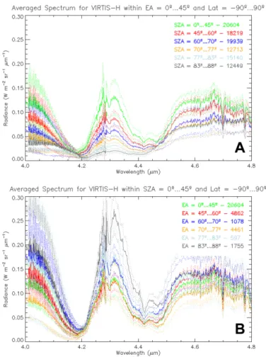
Fig. 1.Averaged spectra taken by VIRTIS-H and for all latitudes during Medium Term Planning covering several orbits of VEx (MTP001 ). Sets of spectra are shown for different intervals of SZA fixing the EA (A), and different intervals of EA fixing the SZA (B).
worse spatial resolution. The VIRTIS-H spectra are subdivided in eight spectral orders, with 432 elements in each one,
cover-ing infrared wavelengths from 1.88 to 5.03 µm (Drossart et al.
2007). We only used the order covering 4.01–5.03 µm (2000–
2500 cm−1) in this work, which includes the strong NLTE CO2
emission at 4.3 µm. The spectral resolution in our order is about 2 cm−1and the sampling step is 1 cm−1which, in contrast to the
CO band at 4.7 µm, inhibits the separation of the CO2rotational
lines and vibrational bands (Gilli et al. 2015). In contrast to the limb data used byGilli et al.(2015), we cannot retrieve vertical
information from this CO2band in nadir geometry since a much
larger spectral resolution would be required.
As observed with limb spectra in Venus (Gilli et al. 2009)
and in limb/nadir sounding in Mars (Formisano et al. 2006;
López-Valverde et al. 2005), the nadir dayside IR spectra around 4.3 µm also exhibit a characteristic double-peak
struc-ture with maxima around 4.28 and 4.32 µm (see Fig. 1, and
the study of nadir observations with VIRTIS-M by Garcia
et al. 2009). These dayside IR spectra are well predicted by NLTE models and are mostly caused by the strong solar
pump-ing at 2.7 µm of the (1001) and (0201) vibrational states
of the major CO2 isotope (López-Valverde et al. 2007). We
use a sophisticated NLTE model of the Venus Atmosphere (Roldán et al. 2000;López-Valverde et al. 2007) to simulate the emerging dayglow emission that would be expected for Venus
at different conditions of observations. In the case of nadir
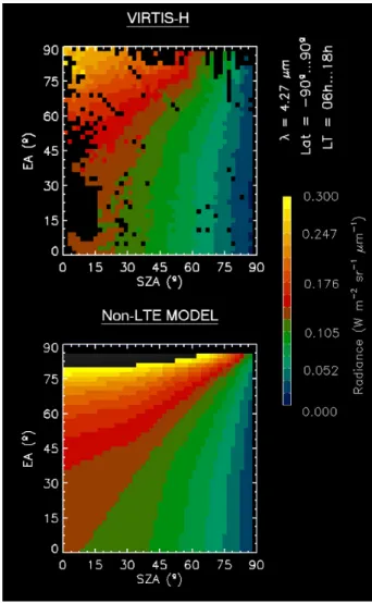
Fig. 2. Comparison between maps SZA-EA of averaged radiance at 4.27 µm from spectra taken by VIRTIS-H and from our NLTE model.
observations, it can be demonstrated that the emerging CO2
spectrum at 4.3 µm mainly comes from the emitting layers
within the range 10−2–10−5 mb (see Sect. 3). Figure 1 shows
two sets of VIRTIS spectra selected to illustrate the impact of the solar zenith angle (SZA) and of the emission angle (EA). The gradual changes show an enhanced emission for larger so-lar illumination (lower SZA) and for a so-larger number of layers contributing to the emission (larger EA). Moreover, the NLTE
forward model not only reproduces the spectral shape (Fig. 1),
but also the variations with SZA and EA with a good agreement.
This is shown in Fig.2at 4.27 µm, a wavelength near the NLTE
emission peak. The agreement between model simulations and measurements is satisfactory, including the SZA and emission
angle variation (Figs. 1 and 2) except at wavelengths beyond
4.34 µm. There, a scattering component from the solar reflexion at the clouds’ tops, or more likely in the mesospheric hazes, is significant, and the model systematically underestimates the ob-served radiance. For this reason, the analysis is focused on the range 4.22−4.34 µm. This NLTE forward model is a key part of our retrieval scheme. This kind of scheme is similar to that used byGilli et al.(2015), and consists of two steps described in more detail in Sect.3.
Fig. 3.Sensitivity expected in emerging NLTE emissions at 4.3 µm for temperature changes of about 1 K.
3. Temperature retrieval and error
As stated in the previous section, we followed a NLTE retrieval scheme previously developed and applied to VIRTIS limb CO
emissions by Gilli et al. (2015). In contrast to the work of
these authors, where two parameters (temperature and CO abun-dance) were derived simultaneously, we only estimated the at-mospheric temperature in this case. The core of the inversion scheme is a NLTE forward model that consists of a line-by-line radiative transfer code and the Venus NLTE model developed
at IAA/CSIC (Roldán et al. 2000;López-Valverde et al. 2007),
which was used to simulate the Venusian emerging infrared day-glow emission for the varied observational conditions of VEx.
Although SZA and EA are the two major parameters defin-ing the emission, the atmospheric temperature may be derived
from these VIRTIS-H spectra since the CO2NLTE nadir
emis-sions still have some sensitivity to temperature (López-Valverde
et al. 2005). We tested our NLTE forward model sensitivity for temperature disturbances of about 20 K at different altitudes, ob-taining similar results at most frequencies within the 4.30 µm
band. These Jacobians, presented Fig. 3, show a peak
sensi-tivity around 5 × 10⁻⁴ mb, with changes in the radiance of
2−3 × 10⁻³W × m−2× sr−1×µm, which is about half the
nomi-nal noise level for a single spectrum. The width of this function describes the vertical resolution of our retrieval, and hence we cannot resolve narrower features like small-scale waves or ther-mal gradients within this broad region. Following the previous work byGilli et al.(2015), we carried out a retrieval of the tem-perature following two steps.
In the first step, every measured spectrum is compared to a pre-computed set of synthetic spectra, at the appropriate SZA
and EA, using a χ2 minimization procedure. This χ2 is
evalu-ated for all the wavelengths in the 4.20–4.35 µm range and is used to define a first-fit spectrum. In the second step of the re-trieval, a linear inversion is performed around this first fit (used
A&A 585, A53 (2016)
Fig. 4. Thermal profiles used as reference for the set of temperature perturbations in vertical coordinates of pressure (A) and kilometers (B). The red curves corresponds to the thermal profiles from the reference at-mosphere VTS3 (Hedin et al. 1983), while the black curve corresponds to an arbitrary isothermal profile. The sensed vertical region for temper-ature perturbations ranging from ±10 to ±60 K is labelled with different line styles.
as reference state close to the real solution) to obtain the best
fit, following the optimal estimation formalism (Rodgers 2000).
The set of synthetic spectra was created with the NLTE forward model for a set of atmospheric profiles and observational con-ditions, with a grid of 11 points in SZA, 11 points in EA, and 13 points in temperature. These 13 temperatures correspond to
perturbations from −60 to+60 K in regular steps of 10 K around
the nominal VTS3 profile (Hedin et al. 1983) between 10−2and
10−5 mb, as shown in Fig. 4 (left panel). An additional set of
13 thermal profiles was also generated and applied to the 121 ob-servational conditions (11 SZA values times 11 EA values), but with an isothermal reference atmosphere. This isothermal case was used to test the impact of the unknown profile shape on the
results, as explained below. Figure 5shows an example of this
two-step retrieval applied to a single VIRTIS-H nadir spectrum.
The whole database of VEx/VIRTIS-H comprised a total of
200, 036 spectra after selecting values of SZA and EA lower
than 80◦ (the signal-to-noise for higher values of SZA and EA
is found to be too low). Despite this restriction, low-quality re-trievals were frequently obtained, hence, additional quality cri-teria were applied. We discarded retrievals where: (a) no clear
single minimum was present in the χ2function; or (b) this
mini-mum was placed at the maximini-mum/minimum temperature
pertur-bation (in our case at ±60 K); or (c) the inversion was possibly outside the linear regime, i.e. the absolute value of the di ffer-ence between the temperatures for best fit and first fit was higher than the step of 10 K used for temperature perturbations (i.e. |TBF− TFF| > 10 K) or this difference was more than twice the
error bars for the best fit. As a result, about a 33% of the nadir spectra were finally discarded and we obtained 133 015 valid re-trievals of dayside temperatures covering more than five years of data.
We averaged the atmospheric temperatures hereby obtained
for a grid of latitude and local time with bins of 5◦ in latitude
and 0.25 h in local time, and chose these values as a com-promise between maximizing the spatial coverage and mini-mizing the errors. The total error in each bin is calculated as
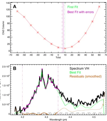
Fig. 5.Model fitting of one VIRTIS-H spectrum. (A) Minimization of χ2 differences for a set of synthetic spectra obtained for 13 different
values of atmospheric temperature in the UMLT region, Tdiststands for
temperature (K) from a fixed value used as reference; (B) synthetic spectrum best fits an individual nadir spectrum taken by the instru-ment VIRTIS-H. The fit is carried out using frequencies ranging 4.20– 4.35 µm. The first-step fit and the residuals are also shown with green and brown lines, respectively (see text.)
σ2 = σ2
SD+ σ
2
Method, where σSDis the standard deviation of the
temperatures within the bin and the methodological error
con-tains two components: the retrieval error (σRet) and the
uncer-tainty from the unknown shape of the thermal profile used in the set of synthetic spectra (σShape). As mentioned above, the actual
shape of the thermal profile is unknown within the range of
al-titudes (pressures, to be precise) actually sounded by this CO2
4.3 µm band. To evaluate the impact that this uncertainty has on
the temperature retrieval, two different profiles were used when
generating the database of pre-computed spectra. One of these
is the VTS3 daytime profile (Hedin et al. 1983), possibly more
appropriate for near-subsolar soundings, and the second one is a colder and isothermal profile, presumably closer to higher SZA and near-terminator conditions. Both profiles were disturbed in a similar way, with 10 K steps within the pressure range of
inter-est, 10−2–10−5mb. Figure4shows these reference atmospheres
in isobaric coordinates (left-hand panel). Nevertheless, a word of caution is needed for comparisons with other results. Our retrieval scheme is well defined in a pressure scale but the ac-tual altitudes may change depending on the acac-tual thermal struc-ture. This is clearly illustrated in the right-hand panel of Fig.4, which is similar to the left-hand panel except in altitude coor-dinates. This profile-shape uncertainty (σShape) turned out to be
larger than the retrieval error (σRet), especially near the
termi-nator (high latitudes, and early morning and late afternoon local times). In addition, the joint contribution or methodological error
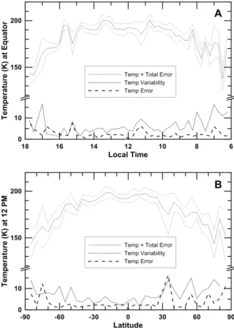
Fig. 6.Comparison for typical errors at the equator A) and at midday B). The averaged temperature along with the total error is shown with continuous lines, while the error due to the variability (standard devi-ation of the mean) and that due to the pure error (retrieval error plus the nominal profile dependent) are shown with dotted and dashed lines, respectively.
(σ2
Method) is usually smaller than the actual atmospheric
variabil-ity (σ2
SD). All these error terms are shown in Fig.6.
4. Results and discussion
After applying specific criteria to discard lower quality retrievals
(see Sect.3), we obtained a total of 133 015 dayside
tempera-tures covering more than five years of data (from 2006/05/14 to
2011/06/05). These errors are typically between 5−10 K with
a slight increase towards the terminator (see Sect. 3). Also, as
explained previously, these temperatures were averaged onto a
grid of latitude and local time with bins of 5◦ in latitude and
0.25 h in local time to maximize the spatial coverage and min-imize errors. The number of spectra or temperatures in most of these boxes varies between 5 and 20, with a few boxes with more than 25 values. The magnitude of the standard deviation within each bin is about 15 K, interpreted to be caused by the atmospheric variability. This is similar to typical noise values. The exception is close to the terminator, where the standard
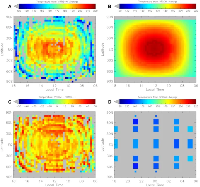
deviation has a small increase, up to 20−25 K. Figure 7A
ex-hibits the obtained 2D horizontal distribution of temperature and
Fig.8 shows the latitude and local time variations (meridional
and zonal scans in the 2D map) at the equator. A strong gradient of temperature of about 55 K is apparent from the warmest area at the subsolar point (around 190–200 K) and decreases to about 140 K at the near terminator.
This result is in qualitative agreement with the Venus’
up-per atmosphere global models. Figure 7 also shows
latitude-local time maps of numerical results from the Venus Thermal
General Circulation Model (VTGCM) by Brecht & Bougher
(2012) (panel B) and its difference from our measurements (C),
while Fig. 8 shows the variations of this model with latitude
(panel A) and with local time (B) around the subsolar point. Their simulations were performed for solar cycle conditions rep-resentative of the VEx data set (near solar minimum). For a co-herent comparison, data from the VTGCM were averaged for the interval 10−2–10−5 mb with our Jacobian functions (see Fig.3)
as well as interpolated onto the same grid of latitude and local
time as VIRTIS-H. Figures7and8 clearly exhibit a colder
at-mosphere than in the VTGCM, with temperatures reaching dif-ferences of 20–25 K near the subsolar point that were smaller away from this point and increasing up to 30 K at the near ter-minator, although our data and retrievals here are noisier. The standard deviation in the VTGCM bins is maximum at the sub-solar point, about 25 K, and smaller, about 15 K, near the termi-nator. Our data presents a plateau around the subsolar point, in contrast to the model that shows a clear maximum in the central point. This difference appears to be above the noise level and it might be the result of atmospheric variability, mostly temporal variability in our data set. This difference has been also observed in limb observations of the CO dayglow with retrieved
tem-peratures lower than the VTGCM in the subsolar region (Gilli
et al. 2015, see Fig. 14). Nightside temperatures from SPICAV (Piccialli et al. 2015) were also averaged for the same pressure
interval as our dayside data (see panel7D), exhibiting a much
colder atmosphere.
A comparison with other temperature measurements is
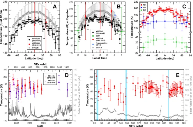
shown in Figs.7and8, and a study of the time evolution in our
data is also indicated in Fig.8. Concerning the temperatures de-rived from the CO dayglow measured by VIRTIS-H in the limb (Gilli et al. 2015) a good agreement is found despite their large error bars (above 40 K). Regarding temperatures from
ground-based observations (Krasnopolsky 2014) a proper comparison
is not possible because of the different vertical layer sensed. And although solar occultation with SOIR show larger error bars (Mahieux et al. 2015a), and their vertical weighting functions are also different, their temperatures agree well with the tendency of our values towards the terminator. On the other hand, the ther-mal gradient between the subsolar and antisolar meridians is of crucial importance to get an accurate evaluation of the SS-AS circulation. Caution must be taken in comparing VIRTIS with SPICAV data, since SPICAV uses altitude as the vertical
co-ordinate. For this reason, we used Fig.4 to infer which is the
corresponding altitude interval sensed for the subsolar tempera-tures of about 190 K (in this case, 100–125 km). Accordingly, SPICAV temperatures for the antisolar region were averaged for the same altitude region. Subsolar and antisolar values
(com-bining VIRTIS and SPICAV data) are presented in Fig.8C and
show a difference of 33 ± 21 K, much lower than the VTGCM
large day-night differences of more than 50 K at a fixed altitude
like 110 km (Brecht & Bougher 2012). However, the
tempera-ture in the nightside varies a lot with altitude within our pressure range and careful model averages should be considered. For
ex-ample, the model differences between the mesopeak on the
day-side (around 110 km) and on the nightday-side (around 104 km) is about 40 K, closer to our day-night gradient.
Finally, we examined long-term and short-term variations in the UMLT region. The time variation of the mean tempera-ture for latitudes 30◦S–30◦N of the subsolar region (10 h–14 h)
A&A 585, A53 (2016)
Fig. 7.Atmospheric temperature in the UMLT of Venus. A) Dayside temperatures inferred from CO2NLTE nadir spectra taken by
VEx/VIRTIS-H; B) dayside temperatures from the VTGCM byBrecht & Bougher(2012) and averaged for the pressure interval 10−2–10−5mb; C) difference
between temperatures from the VTGCM and VIRTIS-H; D) nightside temperatures inferred with stellar radio-occultation data from VEx/SPICAV (Piccialli et al. 2015) and averaged for the pressure interval 10−2–10−5mb.
(Figs.8E). In the case of the long-term behaviour, temperatures
have been also averaged along series of consecutive days cov-ering no more than 40 days, depending on the availability of data. For the short-term behaviour, we only display daily aver-ages. The basic result is that VIRTIS data exhibit a fairly stable behaviour, at least on the dayside hemisphere and on our aver-aged UMLT region. In contrast to the apparent stability exhib-ited for temperatures at midday and evening zones, remarkable variations up to 30 K seem trigger in only one or two days in the subsolar region as shown with blue areas in panel E. These sudden thermal variations are also compared in panels D and E
with the solar radio flux at 10.7 cm (Tobiska et al. 2000), with
no apparent correlation.
5. Conclusions
In this paper, we have measured for the first time the horizontal distribution of the dayside temperatures in the UMLT of Venus
at the pressure interval 10−2–10−5mb. A total of 133 015 dayside temperatures covering more than five years of data have been ob-tained by means of an inversion procedure applied to the NLTE
CO2 dayglow nadir spectra at 4.3 µm, as measured by the
in-strument VIRTIS-H on board VEx. Our dayside temperatures peak is about 195 K in a broad region around the subsolar point, extending to the latitude interval 20◦S–20◦N and to local times
10 h–15 h. This is in contrast to VTGCM results, which peak precisely at the subsolar point and reach 215 K. When there is coincidence, our results are in good agreement with the few previous ground-based and remote sensing measurements avail-able at these altitudes. Our results behave similarly to predic-tions from numerical models (Brecht & Bougher 2012), and de-crease away from the subsolar point, although they exhibit a 25 K colder atmosphere. A gradient of up to 35 K is found be-tween the subsolar and antisolar points when comparing our data with nightside temperatures from SPICAV at the same altitude region (Piccialli et al. 2015). Finally, time evolution shows that UMLT temperatures on Venus are very stable through the years
Fig. 8.Atmospheric temperature at the lower thermosphere of Venus: comparison and time evolution. A) and B) show our temperatures at the subsolar meridian and the equator compared with results from CO NLTE limb spectra (Gilli et al. 2015;Krasnopolsky 2014), solar occultation with SOIR/VEx (Mahieux et al. 2015a), and numerical VTGCM (Brecht & Bougher 2012); C) subsolar (red) and antisolar temperatures (blue) inferred with CO2 NLTE spectra taken by VEx/VIRTIS-H (this work) and with stellar occultation using SPICAV (Piccialli et al. 2015). The
difference between subsolar and antisolar temperatures are shown in green. Antisolar temperatures are averaged for the same altitude region as the pressure layer 10−2–10−5mb at the subsolar meridian (see Fig.4); D) and E) indicate long- and short-time evolution of the temperature, averaged
for consecutive and single days, respectively, as well as for intervals of latitude (30◦
S–30◦
N) and local time (10h–14h shown with red dots, and 14h–16h with purple dots). The solar radio flux at 10.7 cm (Tobiska et al. 2000) is also shown in grey. Sudden changes in temperature are shown in cyan in panel E).
except for several episodes where the subsolar region is shown to vary about 30 K in less than two days by mechanisms yet to be unveiled.
Acknowledgements. J.P. and MA.L-V acknowledge the Spanish MICINN for funding support through the CONSOLIDER program “ASTROMOL” CSD2009-00038 and project AYA2011-23552. J.P. also thanks the JAXA International Top Young Fellowship program, GG thanks CNES postdoc contract and A.P. ac-knowledges funding from the European Union Seventh Framework Programme (FP7/2007−2013) under Grant agreement No. 246556. We also thank J. L. Bertaux and F. Montmessin for their support with VEx/SPICAV.
References
Bougher, S. W., Roble, R. G., & Fuller-Rowell, T. 2002, Washington DC American Geophysical Union Geophysical Monograph Series, 130, 261 Bougher, S. W., Rafkin, S., & Drossart, P. 2006,Planet. Space Sci., 54, 1371 Brecht, A. S., & Bougher, S. W. 2012,J. Geophys. Res. (Planets), 117, 8002 Dickinson, R. E. 1972,J. Atmos. Sci., 29, 1531
Drossart, P., Piccioni, G., Adriani, A., et al. 2007,Planet. Space Sci., 55, 1653 Formisano, V., Maturilli, A., Giuranna, M., D’Aversa, E., & Lopez-Valverde,
M. A. 2006,Icarus, 182, 51
Garate-Lopez, I., García Muñoz, A., Hueso, R., & Sánchez-Lavega, A. 2015, Icarus, 245, 16
Garcia, R. F., Drossart, P., Piccioni, G., López-Valverde, M., & Occhipinti, G. 2009,J. Geophys. Res. (Planets), 114, 0
Gilli, G., López-Valverde, M. A., Drossart, P., et al. 2009, J. Geophys. Res. (Planets), 114, E00B29
Gilli, G., López-Valverde, M. A., Peralta, J., et al. 2015,Icarus, 248, 478 Grassi, D., Migliorini, A., Montabone, L., et al. 2010,J. Geophys. Res., 115,
9007
Hedin, A. E., Niemann, H. B., Kasprzak, W. T., & Seiff, A. 1983,J. Geophys. Res., 88, 73
Keating, G. M., Bertaux, J. L., Bougher, S. W., et al. 1985,Adv. Space Res., 5, 117
Krasnopolsky, V. A. 2014,Icarus, 237, 340
López-Puertas, M., & Taylor, F. W. 2001, in Non-LTE radiative transfer in the atmosphere (World Scientific), eds. M. López-Puertas, & F. W. Taylor, 3 López-Valverde, M. A., López-Puertas, M., López-Moreno, J. J., et al. 2005,
Planet. Space Sci., 53, 1079
López-Valverde, M. A., Drossart, P., Carlson, R., Mehlman, R., & Roos-Serote, M. 2007,Planet. Space Sci., 55, 1757
Mahieux, A., Vandaele, A. C., Bougher, S. W., et al. 2015a,Planet. Space Sci., 113, 309
Mahieux, A., Vandaele, A. C., Robert, S., et al. 2015b,Planet. Space Sci., 113-114, 347
Migliorini, A., Grassi, D., Montabone, L., et al. 2012,Icarus, 217, 640 Piccialli, A., Montmessin, F., Belyaev, D., et al. 2015,Planet. Space Sci., 113,
321
Rodgers, C. D. 2000, Inverse Methods for Atmospheric Sounding – Theory and Practice. Series: Series on Atmospheric Oceanic and Planetary Physics (World Scientific Publishing Co. Pte. Ltd.), 2, 2
Roldán, C., López-Valverde, M. A., López-Puertas, M., & Edwards, D. P. 2000, Icarus, 147, 11
Sonnabend, G., Krötz, P., Schmülling, F., et al. 2012,Icarus, 217, 856 Svedhem, H., Titov, D. V., McCoy, D., et al. 2007,Planet. Space Sci., 55, 1636 Tellmann, S., Pätzold, M., Häusler, B., Bird, M. K., & Tyler, G. L. 2009,J.
Geophys. Res. (Planets), 114, E00B36
Tellmann, S., Häusler, B., Hinson, D. P., et al. 2012,Icarus, 221, 471
Tobiska, W. K., Woods, T., Eparvier, F., et al. 2000,J. Atmos. Solar-Terr. Phys., 62, 1233
Wilquet, V., Fedorova, A., Montmessin, F., et al. 2009,J. Geophys. Res., 114, E00B42