Publisher’s version / Version de l'éditeur:
2010 IEEE Congress on Evolutionary Computation (CEC), pp. 1-8, 2010-07-23
READ THESE TERMS AND CONDITIONS CAREFULLY BEFORE USING THIS WEBSITE. https://nrc-publications.canada.ca/eng/copyright
Vous avez des questions? Nous pouvons vous aider. Pour communiquer directement avec un auteur, consultez la première page de la revue dans laquelle son article a été publié afin de trouver ses coordonnées. Si vous n’arrivez pas à les repérer, communiquez avec nous à [email protected].
Questions? Contact the NRC Publications Archive team at
[email protected]. If you wish to email the authors directly, please see the first page of the publication for their contact information.
NRC Publications Archive
Archives des publications du CNRC
This publication could be one of several versions: author’s original, accepted manuscript or the publisher’s version. / La version de cette publication peut être l’une des suivantes : la version prépublication de l’auteur, la version acceptée du manuscrit ou la version de l’éditeur.
For the publisher’s version, please access the DOI link below./ Pour consulter la version de l’éditeur, utilisez le lien DOI ci-dessous.
https://doi.org/10.1109/CEC.2010.5585951
Access and use of this website and the material on it are subject to the Terms and Conditions set forth at
Evolutionary computation based nonlinear transformations to low
dimensional spaces for sensor data fusion and visual data mining
Valdés, Julio J.
https://publications-cnrc.canada.ca/fra/droits
L’accès à ce site Web et l’utilisation de son contenu sont assujettis aux conditions présentées dans le site LISEZ CES CONDITIONS ATTENTIVEMENT AVANT D’UTILISER CE SITE WEB.
NRC Publications Record / Notice d'Archives des publications de CNRC:
https://nrc-publications.canada.ca/eng/view/object/?id=07ebfb0b-cb80-49f6-9dd7-86896af60593 https://publications-cnrc.canada.ca/fra/voir/objet/?id=07ebfb0b-cb80-49f6-9dd7-86896af60593
Evolutionary Computation Based Nonlinear Transformations to
Low Dimensional Spaces for Sensor Data Fusion and Visual Data
Mining
Julio J. Vald´es, Senior Member, IEEE
Abstract— Data fusion approaches are nowadays needed and
also a challenge in many areas, like sensor systems moni-toring complex processes. This paper explores evolutionary computation approaches to sensor fusion based on unsupervised nonlinear transformations between the original sensor space (possibly highly-dimensional) and lower dimensional spaces. Domain-independent implicit and explicit transformations for Visual Data Mining using Differential Evolution and Genetic Programming aiming at preserving the similarity structure of the observed multivariate data are applied and compared with classical deterministic methods. These approaches are illus-trated with a real world complex problem: Failure conditions in Auxiliary Power Units in aircrafts. The results indicate that the evolutionary approaches used were useful and effective at reducing dimensionality while preserving the similarity struc-ture of the original data. Moreover the explicit models obtained with Genetic Programming simultaneously covered both feature selection and generation. The evolutionary techniques used compared very well with their classical counterparts, having additional advantages. The transformed spaces also help in visualizing and understanding the properties of the sensor data.
I. INTRODUCTION
Data fusion in general and sensor data fusion in particular, are necessary. The progress in sensor and communication technologies demand generic and robust combination of monitored data coming from sensor nodes and networks [1]. It becomes increasingly important in large scale sensor system to make data transmission, storage and interpretation more efficient. In this sense dimensionality reduction [2] and relevant information finding while preserving as much inter-nal properties of the data as possible, becomes a challenging but important goal. The reduction of the dimensionality of the data benefits the application of many processing techniques as it alleviate the curse of dimensionality and makes the application of the methods more efficient and effective. On the other hand, it makes possible the visual interpretation of the data and allows a more direct involving of domain experts and decision makers, in the spirit of Visual Data Mining and Exploratory Analysis. Another important benefits are the reduction of the noise level and redundancies in the data.
Two main approaches are feature selection and feature generation. Whereas in the former the objective is to find (smaller) subsets of the original features with as much
Julio J. Vald´es is with the National Research Council Canada, Institute for Information Technology, 1200 Montreal Rd. Bldg M50, Ottawa, ON K1A 0R6, Canada (phone: 1-613-993-0887; fax: 1-613-993-0215; email: [email protected]).
descriptive or discriminatory power as possible, the later tries to produce new (fewer) features as functions of the original ones, hence creating a new space of dimension equal to the number of created features. Mathematically, feature selection works with subspaces of the original one, whereas feature generation works with new spaces created by transformations of the original. These mappings may be linear, like the classical principal components of factor analysis [3], or nonlinear, which are more flexible and powerful, but also more complex. A generic nonlinear approach to sensor data aggregation was introduced in [4] and applied to real-world complex sensor data from auxiliary aircraft engines. Using classical (deterministic) optimization methods it was shown that a substantial dimensionality reduction can be achieved. This paper extends the study to the use of computational intelligence methods (in particular, evolutionary computa-tion algorithms (EC)) for nonlinear transformacomputa-tions into low dimensional spaces with dimensionality reduction and Visual Data Mining purposes. Differential Evolution (DE) and Genetic Programming (GP) are used to obtain implicit and explicit mappings. The preliminary results show that dimensionality reduction can be achieved at levels totally equivalent to those obtained with classical deterministic methods. Also, feature selection is achieved when using explicit analytic models from which the relevant variables can be readily exposed and their importance quantified. The paper is organized as follows: Section II reviews the use of nonlinear transformations for data fusion with classical meth-ods. Section III introduces two evolutionary approaches for the same purpose (DE and GP). Section IV briefly presents the case study (Auxiliary Power Units (engines) in aircrafts). Section V describes the experimental framework. Section VI presents the results and Section VII the conclusions.
II. NONLINEARSPACETRANSFORMATIONS FOR
INFORMATIONFUSION
The construction of a smaller feature space can be per-formed via a nonlinear transformation that maps the original set of 𝑁 -dimensional objects under study 𝒪 into another space ˆ𝒪 of smaller dimension ˆ𝑑 < 𝑁 . An intuitive metric should be used for Visual Data Mining purposes, besides dimensionality reduction. A feature generation approach of this kind implies information losses and non-linear trans-formations (𝜑 : 𝒪 → ˆ𝒪) are required. This approach has been used for data representation and Visual Data Mining (knowledge and data exploration) [5]. There are essentially
three kinds of spaces generally sought [6]: i) spaces pre-serving the structure of the objects as determined by the original set of attributes or other properties (unsupervised approach), ii) spaces preserving the distribution of an existing class or partition defined over the set of objects (supervised approach), and iii) hybrid spaces. Data structure is one of the most important elements to consider and it can be approached by looking at similarity relationships [7], [8] between the objects, as given by the set of original attributes [5]. From this point of view, transformations𝜑 can be constructed that minimize error measures of information loss [9], based on similarities or distances.
If 𝛿(⃗𝑥, ⃗𝑦) is a dissimilarity measure between any two objects⃗𝑥⃗𝑦 ∈ 𝒪 , and 𝜁(ˆ⃗𝑥, ˆ⃗𝑦) is another dissimilarity measure defined on objects ˆ⃗𝑥, ˆ⃗𝑦 ∈ ˆ𝒪 (ˆ⃗𝑥 = 𝜑(⃗𝑥), ˆ⃗𝑦 = 𝜑(⃗𝑦)), a frequently used error measure associated to the mapping 𝜑 is the Sammon error [9]:
𝒮𝑒= 1 ∑ ⃗ 𝑥∕=⃗𝑦 𝛿(⃗𝑥, ⃗𝑦) ∑ ⃗ 𝑥∕=⃗𝑦 ( 𝛿(⃗𝑥, ⃗𝑦) − 𝜁(ˆ⃗𝑥, ˆ⃗𝑦))2 𝛿(⃗𝑥, ⃗𝑦) (1)
A. Computation of the Nonlinear Space with Classical Meth-ods
In order to optimize Eq. 1 the classical Fletcher-Reeves algorithm (FR) is used, which is a well known technique used in deterministic optimization [10]. It assumes that the function to optimize can be approximated as a quadratic form in the neighborhood of a 𝑁 dimensional point P and exploits the information contained in the partial derivatives of the objective function. This kind of optimization is prone to local extrema entrapment, therefore it is recommended to try different random initial parameter vectors.
The 𝜑 mappings obtained using the previously described approach are implicit, as the images of the transformed objects are computed directly and the algorithm does not provide a function representation. The accuracy of the map-ping depends on the final error obtained in the optimization process. Explicit mappings can however be obtained from these solutions using neural networks, genetic programming (Section III-A), and other techniques. In general 𝜑 is a nonlinear function and in order to compare results from transformations obtained with different algorithms or dif-ferent initializations, a canonical representation is preferred. It can be obtained by performing a principal component transformation 𝒫 after 𝜑, so that the overall transformation is given by the composition
ˆ
𝜑 = (𝜑▪ 𝒫 ) (2)
referred to as the canonical mapping. Since 𝒫 does not change the dimension of the new space, an advantage of the canonical mapping is to make easier the comparison of different solutions. It also contributes to the interpretability of the new variables, as they have a monotonic distribution of the variance. The images of the mapped objects can be
used for the construction of a 3D model (e.g. using virtual reality), for visual data mining and data exploration (pattern detection, cluster assessment, etc), as in this paper.
III. COMPUTATION OF THENONLINEARSPACE WITH
COMPUTATIONALINTELLIGENCEMETHODS
This task can be performed also using evolutionary com-putation methods.
1) Differential Evolution: Differential Evolution [11], [12] is a kind of evolutionary algorithm working with real-valued vectors, and it is relatively less popular than genetic algorithms. However, it has proven to be very effective in the solution of complex optimization problems [13], [14]. Like other EC algorithms, it works with populations of individual vectors (real-valued), and evolves them. Many variants have been introduced, but the general scheme is as follows:
step 0 Initialization: Create a population𝒫 of random vec-tors in ℜ𝑛, and decide upon an objective function 𝑓 : ℜ𝑛 → ℜ and a strategy 𝒮, involving vector differentials.
step 1 Choose a target vector from the population⃗𝑥𝑡∈ 𝒫. step 2 Randomly choose a set of other population vectors 𝒱 = {⃗𝑥1, ⃗𝑥2, . . .} with a cardinality determined by strategy 𝒮.
step 3 Apply strategy 𝒮 to the set of vectors 𝒱 ∪ {⃗𝑥𝑡} yielding a new vector⃗𝑥𝑡′.
step 4 Add 𝑥⃗𝑡 or 𝑥⃗𝑡′ to the new population according to the value of the objective function 𝑓 and the type of problem (minimization or maximization). step 5 Repeat steps 1-4 to form a new population until
termination conditions are satisfied.
There are several variants of DE which can be classified using the notation𝐷𝐸/𝑥/𝑦/𝑧, where 𝑥 specifies the vector to be mutated, 𝑦 is the number of vectors used to compute the new one and 𝑧 denotes the crossover scheme. Let 𝐹 be a scaling factor, 𝒞𝑟 ∈ ℜ be a crossover rate, 𝐷 be the dimension of the vectors, 𝒫 be the current population, 𝑁𝑝 = 𝑐𝑎𝑟𝑑(𝒫) be the population size, ⃗𝑣𝑖, 𝑖 ∈ [1, 𝑁𝑝] be the vectors of 𝒫, ⃗𝑏𝒫 ∈ 𝒫 be the population’s best vector w.r.t. the objective function 𝑓 and 𝑟, 𝑟0, 𝑟1, 𝑟2, 𝑟3, 𝑟4, 𝑟5 be random numbers in (0, 1) obtained with a uniform random generator function𝑟𝑛𝑑() (the vector elements are ⃗𝑣𝑖𝑗, where 𝑗 ∈ [0, 𝐷)). Then the transformation of each vector ⃗𝑣𝑖 ∈ 𝒫 is performed by the following steps:
step 1 Initialization:𝑗 = (𝑟 ⋅ 𝐷), 𝐿 = 0 step 2𝑤ℎ𝑖𝑙𝑒(𝐿 < 𝐷)
step 3𝑖𝑓 ((𝑟𝑛𝑑() < 𝒞𝑟)∣∣𝐿 == (𝐷 − 1))
/* create a new trial vector. For example, as: */ ⃗𝑡𝑖𝑗= ⃗𝑏𝒫𝑗+ 𝐹 ⋅ (⃗𝑣𝑟1𝑗+ ⃗𝑣𝑟2𝑗− ⃗𝑣𝑟3𝑗− ⃗𝑣𝑟4𝑗) step 4𝑗 = (𝑗 + 1) mod 𝐷
step 5𝐿 = 𝐿 + 1 step 6 goto 2 step 7 stop
Many particular strategies have been proposed and they differ in the way the trial vector is constructed (step 3 above). The
ones used in this paper are (see Table. I): 𝐷𝐸/ 𝑏𝑒𝑠𝑡/2/𝑏𝑖𝑛 𝑡𝒫 𝑖𝑗 = 𝑣𝑏𝑗𝒫 + 𝐹 × (𝑣𝑟𝒫1𝑗+ 𝑣 𝒫 𝑟2𝑗− 𝑣 𝒫 𝑟3𝑗− 𝑣 𝒫 𝑟4𝑗) 𝐷𝐸/ 𝑟𝑎𝑛𝑑/2/𝑏𝑖𝑛 𝑡𝒫 𝑖𝑗 = 𝑣𝑟𝒫5𝑗+ 𝐹 × (𝑣 𝒫 𝑟1𝑗+ 𝑣 𝒫 𝑟2𝑗− 𝑣 𝒫 𝑟3𝑗− 𝑣 𝒫 𝑟4𝑗) 𝐷𝐸/ 𝑟𝑎𝑛𝑑/1/𝑒𝑥𝑝 𝑡𝒫 𝑖𝑗 = 𝑣𝑟𝒫3𝑗+ 𝐹 × (𝑣 𝒫 𝑟1𝑗− 𝑣 𝒫 𝑟2𝑗) 𝐷𝐸/ 𝑏𝑒𝑠𝑡/1/𝑒𝑥𝑝 𝑡𝒫 𝑖𝑗 = 𝑣𝑏𝑗𝒫 + 𝐹 × (𝑣𝑟𝒫1𝑗− 𝑣 𝒫 𝑟2𝑗) 𝐷𝐸/ 𝑏𝑒𝑠𝑡/2/𝑒𝑥𝑝 𝑡𝒫 𝑖𝑗 = 𝑣𝑏𝑗𝒫 + 𝐹 × (𝑣𝑟𝒫1𝑗+ 𝑣 𝒫 𝑟2𝑗− 𝑣 𝒫 𝑟3𝑗− 𝑣 𝒫 𝑟4𝑗) 𝐷𝐸/ 𝑟𝑎𝑛𝑑 − 𝑡𝑜 − 𝑏𝑒𝑠𝑡/1/𝑒𝑥𝑝 𝑡𝒫 𝑖𝑗 = 𝑣𝑖𝑗𝒫+ 𝐹 × (𝑣𝑏𝑗𝒫 + 𝑣𝑖𝑗𝒫− 𝑣𝒫𝑟1𝑗− 𝑣 𝒫 𝑟2𝑗) (3) where 𝑡𝒫
𝑖𝑗 is a new trial vector and𝑏 is the index to the best vector ⃗𝑏𝒫. Some of them, like the𝐷𝐸/𝑏𝑒𝑠𝑡/2/𝑏𝑖𝑛 have been reported as producing good results in a wide variety of test problems [14].
When using DE for solving the nonlinear mapping prob-lem described by Eq.1 the dimension of the vectors in the DE algorithm was set to𝐷 = 𝑐𝑎𝑟𝑑(𝒪)× ˆ𝑑 in order to construct a representation in which each DE vector provides a candidate solution to Eq.1, which clearly be an implicit mapping.
A. Genetic Programming
Genetic programming (GP) techniques aim at evolving computer programs. They are an extension of the Genetic Algorithm introduced in [15] and further elaborated in [16], [17] and [18]. The algorithm starts with a set of ran-domly created computer programs. This initial population goes through a domain-independent breeding process over a series of generations. Genetic programming combines the expressive high level symbolic representations of computer programs with the search efficiency of the genetic algorithm. Those programs which represent functions are of particu-lar interest and can be modeled as 𝑦 = 𝐹 (𝑥1, ⋅ ⋅ ⋅ , 𝑥𝑛), where (𝑥1, ⋅ ⋅ ⋅ , 𝑥𝑛) is the set of independent or predictor variables, and𝑦 the dependent or predicted variable, so that 𝑥1, ⋅ ⋅ ⋅ , 𝑥𝑛, 𝑦 ∈ ℝ, where ℝ are the reals. The function 𝐹 is built by assembling functional subtrees using a set of predefined primitive functions (the Function Set), defined be-forehand. In general terms, the model describing the program is given by𝑦 = 𝐹 (⃗𝑥), where 𝑦 ∈ ℝ and ⃗𝑥 ∈ ℝ𝑛. Most imple-mentations of genetic programming for modeling fall within this paradigm but for some problems vector functions are required. A GP based approach for finding vector functions was presented in [19]. In these cases the model associated to the evolved programs is ⃗𝑦 = 𝐹 (⃗𝑥), which allows for the simultaneous estimation of several dependent variables ⃗𝑦 from a set of independent variables ⃗𝑥. Note that these are
notmulti-objective problems, but problems where the fitness function depends on vector variables. The mapping problem between vectors of two spaces of different dimension (𝑛 and 𝑚) is one of that kind. In this case a transformation like 𝜓 : ℝ𝑛 → ℝ𝑚, mapping vectors⃗𝑥 ∈ ℝ𝑛 to vectors⃗𝑦 ∈ ℝ𝑚 would allow a reformulation of Eq. 1:
𝒮𝑒= 1 ∑ 𝑖<𝑗𝛿𝑖𝑗 ∑ 𝑖<𝑗(𝛿𝑖𝑗− 𝑑(⃗𝑦𝑖, ⃗𝑦𝑗)) 2 𝛿𝑖𝑗 , (4) where ⃗𝑦𝑖= 𝜓(⃗𝑥𝑖), ⃗𝑦𝑗= 𝜓(⃗𝑥𝑗).
The evolution has to consider populations of forests such that the evaluation of the fitness function depends on the set of trees within a forest [19]. In these cases, the cardinality of any forest within the population is equal to the dimension of the target space 𝑚.
Gene Expression Programming (GEP) [20], [21] is one of the many variants of GP and has a simple string represen-tation. In the GEP algorithm, the individuals are encoded as simple strings of fixed length with a head and a tail, referred to as chromosomes. Each chromosome can be composed of one or more genes which hold individual mathematical ex-pressions that are linked together to form a larger expression. For the research described in this paper, the extension of the GEP algorithm which supports vector functions was used [19]. The GEP implementation is an extension to the ECJ System [22].
When genetic programming is used for solving Eq. 4 by estimating𝜓 explicitly, the terminal set for the GP algorithm may become large (potentially very large) if the dimension of the original space (the number of attributes of the data vectors) is large and the function set is rich. This poses a big challenge to the GP search process, as the search space is huge (perhaps infinite) whereas the number of functions generated during the evolutionary process is necessarily is a tiny fraction of it. However, there are important advantages of GP solutions to Eq. 4 if they provide a reasonable low error level. The explicit nature of the solution makes it a
transparent model rather than a black-box one, which is the case of neural networks, svm’s and other computational intelligence methods. On the other hand, the union of the set of arguments of the vector equations associated to the mapping 𝜓 provides a subset of the original variables found as relevant, since they are the chosen ones for building the GP model equations. Of no smaller advantage is the fact that by retaining not a single, but a set of k-best GP solutions, an ensemble model (committee of experts) can be built. In the same way, the solutions can be boosted or jointly used with a variety of schemes. Yet another potential advantage is a quantitative assessment of the importance of the selected variables, which is given by the elements of the Jacobian matrix as a sensitivity measure.
𝐽𝜓(𝑥1, ⋅ ⋅ ⋅ , 𝑥𝑁) =
∂(𝑦1, ⋅ ⋅ ⋅ , 𝑦𝑑ˆ) ∂(𝑥1, ⋅ ⋅ ⋅ , 𝑥𝑁)
(5) IV. A CASESTUDY: AUXILIARYPOWERUNITSENSOR
DATAFUSION
The Auxiliary Power Unit(APU) engines on commercial aircraft provide electrical power and air conditioning in the cabin prior to the starting of the main engines and also supply the compressed air required to start the main engines when the aircraft is ready to leave the gate. APUs are highly reliable but they occasionally fail to start due to failures of the
APU starter motor. When this happens, additional equipment such as generators and compressors must used to replace APU’s functionalities, which implies significant costs, delays or flight cancellation. Accordingly, airlines are very much interested in monitoring the health of the APU starter motors and proceed with preventive maintenance whenever a failure is suspected. The data comes from sensors installed at strategic locations in the APU which monitors various phases of operation. The ultimate objective is to develop predictive models that can accurately determine the remaining useful life of the starter motors. A generic methodology to tackle this problem was proposed by [23] but non-linear data fusion could help in further improve the results obtained and also facilitate the visualization and interpretation of the data.
The dataset comes from APU starting reports containing 18 original attributes (5 symbolic, 11 numeric, and 2 for date and time of the event) collected around each occurrence of component failures. The analysis is based on data generated between a certain starting date prior to the failure. Statisti-cal, time-series, and signal processing filters on the initial 11 numerical sensor measurements produced an additional collection of188 new variables (features) for a total of 198 numerical variables (the dimension of the original space) and 238 time-stamp instances. With such a highly dimensional space, it is impossible to visualize the characteristics of the APU sensor data.
V. EXPERIMENTALSETTINGS
The data used come from a fleet of 35 commercial Airbus 320 series aircraft collected over a period of 10 years. ACARS (Aircraft Communications Addressing and Reporting System) Auxiliary Power Unit starting reports were made available. Among them, an example of an APU was used for experimentation. Eq. 2 was used for computing new3-D spaces by nonlinear transformation of the original 198-D space of the observed and derived sensor data (via Eq. 1), for 238 time observations. The dissimilarity measure used has the form
𝛿(⃗𝑥, ⃗𝑦) = 1
𝑆(⃗𝑥, ⃗𝑦)− 1 (6) where⃗𝑥, ⃗𝑦 are any two vectors in the original p-dimensional space of sensor information and𝑆(⃗𝑥, ⃗𝑦) is Gower’s similarity coefficient [24] which for numeric variables is
𝑆(⃗𝑥, ⃗𝑦) = 𝑝 ∑ 𝑖=1 1 − ∣ 𝑥𝑖− 𝑦𝑖∣ 𝑅𝑎𝑛𝑔𝑒(𝑖) (7) where 𝑥𝑖, 𝑦𝑖 are the corresponding i-th vector components. A priori, there is no univocal indication about how many new dimensions are required in order to achieve a good similarity preservation between the original sensor space and the reduced target space for an arbitrary dataset. That is, how many dimensions would ensure an acceptable low mapping error. In the present case three dimensional target spaces were tried, as they would allow a visual inspection of the transformed sensor data obtained by different algorithms. In the transformed spaces, the Euclidean distance was used as
the dissimilarity measure. These general settings were the ones used in [4] and were kept the same across the mapping methods used in this paper. The following subsections cover those settings specific to the individual algorithms
A. Classical Optimization Settings
For the Fletcher-Reeves method, the settings were those described in [4]:10 initial random configurations in the target space were tried when computing𝜑. The best mapping errorˆ solution was kept (in order to cope with local minima).
B. Differential Evolution Settings
Table I shows the experimental settings used for different runs of the DE algorithm. For every DE run, the 10 best chromosomes were retrieved. Population size was fixed to 100 vectors of length 714 (238 objects whose image in a 3-D space require 3 coordinates). The maximum number of generations was set to 15000 as well as a Sammon error threshold of0.014. The idea was to asses the DE capabilities to approximate error levels of those obtained with classical methods like FR for the same data.
TABLE I
EXPERIMENTAL SETTINGS FOR THEDIFFERENTIALEVOLUTION ALGORITHM(DE-FR). 3DAND1DSPACES WERE COMPUTED
Parameter Values F {0.2, 0.3, 0.4, 0.5, 0.6, 0.7, 0.8} Cross-over Rate {0.3, 0.4, 0.5, 0.6, 0.7, 0.8, 0.9} Population Size {100} Strategies 𝐷𝐸/𝑏𝑒𝑠𝑡/2/𝑏𝑖𝑛, 𝐷𝐸/𝑟𝑎𝑛𝑑/2/𝑏𝑖𝑛, 𝐷𝐸/𝑟𝑎𝑛𝑑/1/𝑒𝑥𝑝, 𝐷𝐸/𝑏𝑒𝑠𝑡/1/𝑒𝑥𝑝, 𝐷𝐸/𝑏𝑒𝑠𝑡/2/𝑒𝑥𝑝, 𝐷𝐸/𝑟𝑎𝑛𝑑 − 𝑡𝑜 − 𝑏𝑒𝑠𝑡/1/𝑒𝑥𝑝 Number of Trials 5
A total of 1470 runs covered the experimental settings discussed above, producing a total of 14700 candidate new spaces, as for each run the 10 best vectors were retained. From these first round of results, some few were selected for further exploration (see Section VI-B).
C. Genetic Programming Settings
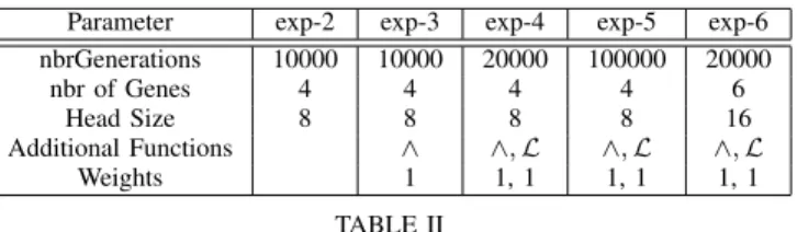
The ECJ-GEP genetic programming experiments were performed using a population sizes of1000 individuals. 100 different random seeds were used for each experiment and the best individual found was kept for each run. The total number of GP experiments was 500. The Function Set was composed by a Basic Set composed of arithmetic functions: {+, −, ∗, /} with weights given by {2, 1, 1, 1} and additional functions like the power (𝑥 ∧ 𝑦 = 𝑥𝑦) and the Logistic (ℒ(𝑥) = 1/(1 + 𝑒−𝑥)) were used in some cases as shown in Table. II.
The remaining algorithm parameters were fixed at the following suggested values [21]: genes/chromosome = 5, gene headsize = 5, elitism = 3 individuals, constants = allowed (in[−1, 1]), probabilities: inversion = 0.1, mutation = 0.044, istransposition = 0.1, ristransposition-prob = 0.1, onepointrecomb-prob = 0.3, twopointrecomb-prob = 0.3,
Parameter exp-2 exp-3 exp-4 exp-5 exp-6 nbrGenerations 10000 10000 20000 100000 20000 nbr of Genes 4 4 4 4 6 Head Size 8 8 8 8 16 Additional Functions ∧ ∧, ℒ ∧, ℒ ∧, ℒ Weights 1 1, 1 1, 1 1, 1 TABLE II
EXPERIMENTAL SETTINGS FOR DIFFERENTGENETICPROGRAMMING EXPERIMENTS(500IN TOTAL).
generecomb-prob = 0.1, genetransposition-prob = 0.1, rnc-mutation= 0.01, dc-mutation-prob = 0.044, dc-inversion= 0.1, dc-istransposition = 0.1.
VI. RESULTS
A. Mapping with classical deterministic methods
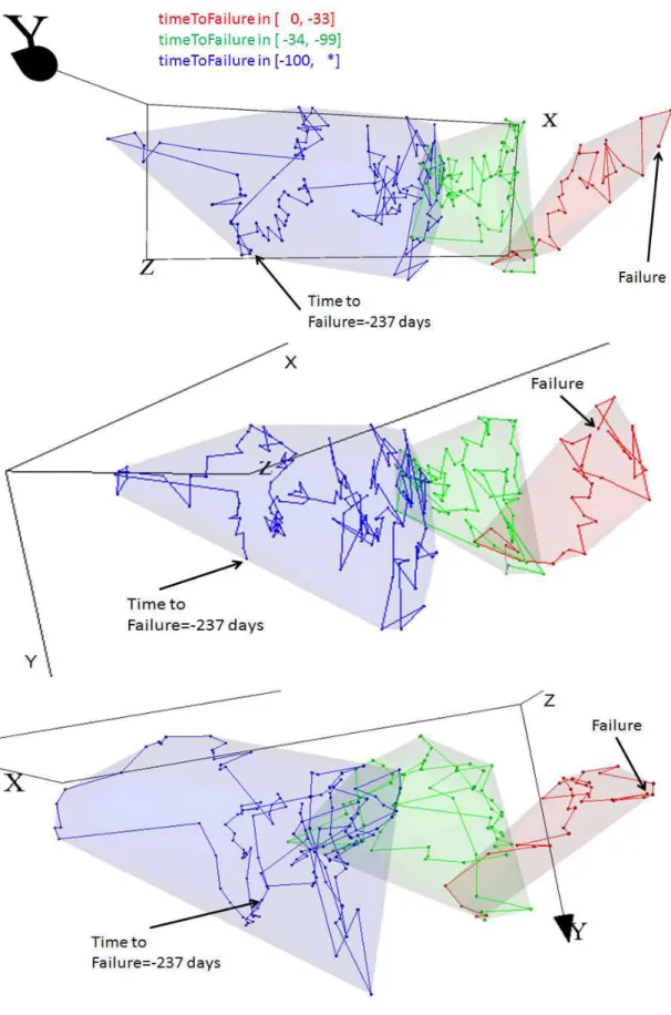
The implicit canonical 3-D mapping of the 198-D vectors (238 in total), corresponding to the APU-1 engine data obtained in [4] is shown in Fig. 1(Top). It is impossible to represent a 3D model on hard media. Therefore fixed snapshots of the actual 3D volume are displayed on the figure. When comparing them it should be remembered that the orientation of the coordinate axis is irrelevant as distance is invariant to rotation.
The small mapping error obtained (0.01315), indicates that despite of the large amount of sensor space compression due to nonlinear dimensionality reduction, the amount of information lost is small. Therefore, the new 3-D space pro-vides a reasonable representation of the overall data structure from the point of view of the preservation of the similarity relationships defined by the original sensor variables.
For comparison purposes, the vectors have been classified into three categories (1: timeToFailure∈ (−∞, −100] days, 2: timeToFailure ∈ [−99, −34] days, 3: timeToFailure ∈ [−33, 0] days), as was done in [4], where transparent closed surfaces wrapping the vectors corresponding to the given classes were added ( Fig. 1). It is important to recall that the computed mappings are unsupervised, therefore this time-to-failure based class information was not used in the process by any of the methods considered. However, the similarity preservation space recognizes well the time evolution of the APU engine status from a far-from-failure states to close-to-failure situations.
From the point of view of the time evolution, a more detailed view is provided by a 3-D polyline joining con-secutive observations starting from the initial vector (237 days before failure), to the final one at failure time. This polyline represents the trajectory of the198 individual time series from the original sensor space and enables a better understanding of the system’s evolution as failure contribut-ing factors cumulate and grow in influence on the process. The X-axis in the canonical nonlinear 3-D space (the one with the largest variance), clearly shows the time evolution of the failure classes: timeToFailure∈ (−∞, −100] days is located at the low values end, whereas the timeToFailure
∈ [−99, −34] days and timeToFailure ∈ [−33, 0] classes follows as the X-values increase. Therefore, the nonlinear X-axis represents an ’aging factor’ of the system. The same convention was used for representing the DE and GP results.
B. Differential Evolution Results
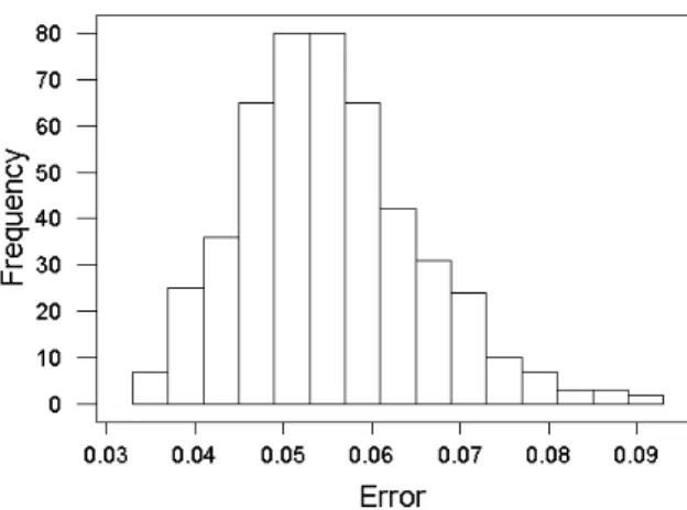
The overall distribution of the mapping error for the 14700 DE-computed new spaces, is shown in Fig. 2. The distribution is bimodal and highly skewed towards low error
Fig. 2. Mapping error distribution for the spaces obtained with Differential Evolution in 15, 000 or less generations.
values, clearly indicating that the overwhelming majority of the spaces obtained are of good quality and that the DE algorithm is robust. The error range is [0.0140, 4.0546] with a median of 0.0264, which is in the order of the best solution obtained with the classical FR algorithm (0.01314). Considering the high dimensionality of the DE vectors (714) this behavior is remarkable. In particular, 267 solutions achieve the error level threshold of 0.014 in 15, 000 or less generations. For these, the distribution of the actual number of generations needed is shown in Fig. 3, which
Fig. 3. Distribution of the number of generations required for the spaces obtained with Differential Evolution to achieve an error threshold of 0.014 in 15, 000 or less generations.
has a bimodal character with modes located around 7, 500 and 13, 000 generations. Most of the runs leading to low mapping error models required less than10, 000 generations.
Fig. 1. ℝ198
→ ℝ3
mapping of the APU data. A 3D polyline links consecutive points along the original 198-dimensional time series from the starting point (Time to Failure = -237) to the last (Time to Failure = 0). Semi-transparent surfaces wrap the three main classes: Time to Failure within 33 days or less, within 33 and 100 days and more than 237 days. The classes are reasonably well distinguished in the 3D space resulting from the nonlinear information fusion process. Top: Space obtained with the classical Fletcher-Reeves method (Error = 0.01315). Middle: Space obtained with Differential Evolution (Error = 0.01315). Bottom: Space obtained with Genetic Programming (Error = 0.0338).
Among these, some converged rapidly to the error threshold in less than 5, 000 generations. In particular, one achieved the error threshold in 4163 generations and was allowed to continue evolving. At 10336 generations it achieved an error of 0.01315, which is the same as the one obtained with the FR method. Considering the high dimensionality of the DE vector space, the fact that many solutions come close to the best result obtained with a classic technique which exploits the knowledge of the partial derivatives of the objective function (which DE does not) is remarkable. The resulting 3D space corresponding to that model is shown in Fig. 1(Middle). The effect of various DE parameters considered on the convergence towards accurate mappings is shown in Table III.
DE Strategy Freq F Freq Crossover Rate Freq DE/best/1/exp 85 0.4 67 0.9 83 DE/rand-to-best/1/exp 63 0.5 61 0.8 55 DE/best/2/exp 44 0.3 57 0.6 44 DE/best/2/bin 28 0.2 43 0.7 38 DE/rand/1/exp 25 0.6 28 0.5 27 DE/rand/2/bin 22 0.7 11 0.3 11 ————- - - - 0.4 9 TABLE III
DISTRIBUTION OF THEDECONTROLLING PARAMETERS FOR THE MODELS WITH MAPPING ERROR UNDER THE0.014THRESHOLD.
The𝐷𝐸/𝑏𝑒𝑠𝑡/1/𝑒𝑥𝑝 and the 𝐷𝐸/𝑟𝑎𝑛𝑑−𝑡𝑜−𝑏𝑒𝑠𝑡/1/𝑒𝑥𝑝 strategies were clearly more prone to drive the evolutionary process towards regions of the search space were high accurate mappings are found. 𝐹 factors are in the [0.3, 0.5] range and Crossover ratios larger than 0.5 lead to good results. Main features of the data distribution in the new space, like the relative ordering and trend of the broad classes defining the system’s state according to the Time to Failure (a variable not considered in the computation of the mapping), are clearly expressed in Fig. 1(Middle) as well as the location of the end states (from −237 days to the failure point). These results show that DE is capable of performing at a level comparable to classical deterministic optimization in providing suitable low dimension implicit mappings.
C. Genetic Programming Results
The general behavior of the mapping error for all GP experiments is shown in Fig. 4. The distribution is skewed towards the low error values which is a good behavior for the algorithm. The error range is [0.03382, 0.09027] with mean and median of0.05532 and 0.05450 respectively. This error range is considerably smaller than the one obtained with DE after almost three times more runs. However, DE was capable to achieve a minimum equal to the one obtained with the FR method, whereas the best GP result was 0.0338 (within experiment 5), which is two times larger. The breakdown of the error values for the individual experiments is shown in the boxplots of Fig. 5. There is not much variation between the results produced by experiments2 and 3 which
Fig. 4. Error distribution for the Genetic Programming experiments.
Fig. 5. Mapping error distributions for the GP experiments (See Table. II).
differ in the number of genes (allowing larger mathematical expressions) and in the introduction of the power function. However, performance improves by increasing the number of generations (more search) and the addition of the logistic function as shown by experiments4 and 5. Experiment 6, was conceived as a derivation of4 in the sense of providing room for forming longer and more complex expressions (increasing the number of genes and the chromosome head size). The performance improvement of experiment 5 with respect to 6 suggests that not too large or complex expressions are necessary beneficial. The results of experiment 5 seems to indicate that the amount of search made is the crucial factor (exps 4 and 5 differ only in the number of generations). Not only its mean, median, minimum and maximum are shifted towards lower error values, but also the interquartile range is smaller than in all other experiments. The best GP model representing the explicit mapping𝜓 is given by Eq. 8. When used in Eq. 4 the resulting 3D space is shown in Fig. 1(Bottom) with a mapping error of 0.0338. This error, although more than two times larger than those of FR and DE is still small enough as to represent a small information loss. The main characteristics of the associated 3D space in terms of the distribution of the time-to-failure classes and the location of the start and end states of the process
(Time to Failure −237 days and Time to failure 0), are the same as what is obtained with the other two methods. However with GP there is the additional advantage of having an analytical model (white box) in contradistinction with the implicit mappings, black-box models given by FR and DE.
𝜓𝑥=(((𝑣186/𝑣170) + (𝑣196/𝑣170)) +(((𝑣75− (𝑣80− 𝑣170)) +((𝑣90/𝑣155) + 𝑣191))/𝑣90)) +((𝑣90+ (𝑣10+ (𝑣175+ 𝑣165)))/𝑣71) 𝜓𝑦=(((ℒ((𝑣85+ 𝑣108)/(𝑣26+ 𝑣165)) + 𝑣38) (8) +ℒ(ℒ((6.811566/𝑣55) − (𝑣181/𝑣117)))) + ℒ(𝑣52)) +ℒ(𝑣118) 𝜓𝑧=((ℒ(𝑣14/𝑣94)/𝑣159)ℒ(ℒ(𝑣33))+ (1/ℒ(𝑣145/𝑣137)) +ℒ(𝑣125/(((𝑣148− 𝑣78) + (𝑣184∗ 𝑣173)) +(𝑣45∗ 𝑣197))) + ℒ(ℒ(𝑣103))
With new data, their images in the new space can be directly obtained by applying Eq. 8. Since the mappings obtained with FR and DE are implicit, it is necessary to merge the new data with the previous and recompute Eq. 1 every time. Another important side result of the GP approach is the feature selection that occurs as part of the evolutionary process. From the original198 attributes defining the original space, only 35 appear as arguments of the 𝜓 functions, meaning that the main similarity structure of the data can be represented with only 17.7% of the original variables, which is also an important dimensionality reduction per se. In terms of search effort, Eq. 8 was found at generation 99, 409. However, another solution obtained with the settings of experiment 4 achieved a mapping error of 0.03890 after 19225 generations, involving 42 variables. This is a fairly equivalent result but requiring only19% of the evolutionary effort. GP can perform comparable to classical deterministic optimization in providing low dimension explicit mappings. The advantage is that both dimensionality reduction and feature selection can be made (not possible with FR or DE).
VII. CONCLUSIONS
Nonlinear unsupervised transformation approaches to data fusion were applied to a case study from the aerospace domain. Experiments for dimensionality reduction were con-ducted, indicating that nonlinear transformations are effective to reduce dimensionality while preserving the structure of the original data and relevant information. The results also demonstrated that the transformed spaces help in understand-ing the characteristics of the sensor data. EC techniques proved to compare well with classical methods, with the extra advantage of providing white box models which allows simultaneous feature selection and generation. However, EC solutions are more expensive that their classical counterparts. The results suggest that relationships could be established between the nonlinear variables of the transformed spaces with the time to failure of the APU unit, which will be further investigated.
REFERENCES
[1] H. Durrant-Whyte, “Data fusion in sensor networks,” in Proc. IEEE
International Conference on Video and Signal Based Surveillance AVSS ’06, 2006, pp. 39–39.
[2] I. Fodor, “A survey of dimension reduction techniques,” Lawrence Livermore National Lab., CA (US), Tech. Rep., 2002.
[3] H. H. Harman, Modern Factor Analysis. University Of Chicago Press; 3 edition, 1976.
[4] J. Vald´es, S. Letourneau, and C. Yang., “Data fusion via nonlinear space transformations,” in Proceedings of the First International
Conference on Sensor Networks and Applications (SNA-2009). San Francisco, USA.: International Society for Computers and Their Ap-plications (ISCA), November 4-6 2009.
[5] J. Vald´es, “Virtual reality representation of information systems and decision rules: an exploratory technique for understanding data knowl-edge structure,” in Lecture Notes in Artificial Intelligence, LNAI. Springer-Verlag, 2003, vol. 2639, pp. 615–618.
[6] J. Vald´es and A. Barton, “Virtual reality spaces for visual data mining with multiobjective evolutionary optimization: Implicit and explicit function representationsmixing unsupervised and supervised properties,” in Proceedings of the IEEE Congress of Evolutionary
Computation, 2006, pp. 592–598.
[7] L. Chandon and S. Pinson, Analyse typologique. Th´eorie et
applica-tions. Masson, 1981.
[8] I. Borg, Multidimensional similarity structure analysis. New York, NY, USA: Springer-Verlag New York, Inc., 1987.
[9] J. W. Sammon, “A nonlinear mapping for data structure analysis,”
IEEE Trans. Comput., vol. 18, no. 5, pp. 401–409, 1969.
[10] W. Press, S. Teukolsky, W. Vetterling, and B. Flannery, Numerical
Recipes in C, 2nd ed. Cambridge, UK: Cambridge University Press, 1992.
[11] R. Storn and K. Price, “Differential evolution-a simple and efficient adaptive scheme for global optimization over continuous spaces.” ICSI, Tech. Rep. tr-09012, 1995.
[12] K. V. Price, R. M. Storn, and J. A. Lampinen, Differential Evolution.
A Practical Approach to Global Optimization., ser. Natural Computing Series. Springer Verlag, 2005.
[13] S. Kukkonen and J. Lampinen, “An empirical study of control parame-ters for generalized differential evolution.” Kanpur Genetic Algorithms Laboratory (KanGAL), Tech. Rep. 2005014, 2005.
[14] R. G¨𝑎mperle, S. D. M¨𝑢ller, and P. Koumoutsakos, “A parameter study for differential evolution.” [Online]. Available: citeseer.ist.psu. edu/526865.html
[15] J. Koza, “Hierarchical genetic algorithms operating on populations of computer programs.” in Proceedings of the 11th International
Joint Conference on Artificial Intelligence. San Mateo, CA. Morgan Kaufmann, 1989, pp. 768–774.
[16] ——, Genetic programming: On the programming of computers by
means of natural selection., MIT Press, 1992.
[17] ——, Genetic programming ii: Automatic discovery of reusable
pro-grams., MIT Press, 1994.
[18] J. Koza, D. Andre, and M. Keane, Genetic programming ii: Automatic
discovery of reusable programs., Morgan Kaufmann, 1999. [19] J. Vald´es, A. Barton, and R. Orchard, “Exploring medical data using
visual spaces with genetic programming and implicit functional map-pings,” in Proceedings of the Genetic and Evolutionary Computation.
GECCO 2007 Conference, London, July 7-11 2007.
[20] C. Ferreira, “Gene expression programming: A new adaptive algorithm for problem solving,” Journal of Complex Systems, vol. 13, no. 2, pp. 87–129, 2001.
[21] ——, Gene Expression Programming: Mathematical Modeling by an
Artificial Intelligence, Springer Verlag, 2006.
[22] S. Luke, L. Panait, G. Balan, S. Paus, Z. Skolicki, E. Popovici, J. Harrison, J. Bassett, R. Hubley, , and A. Chircop, ECJ, A
Java-based Evolution Computing Research System, Evolutionary Computation Laboratory, George Mason University., March 2007. [Online]. Available: http://www.cs.gmu.edu/∼eclab/projects/ecj/ [23] S. L´etourneau, C. Yang, and Z. Liu, “Improving preciseness of time to
failure predictions: Application to APU starter,” in Proceedings of the
1st International Conference on Prognostics and Health Management, Denver, Colorado, USA, October 2008.
[24] J. C. Gower, “A general coefficient of similarity and some of its properties,” Biometrics, vol. 1, no. 27, pp. 857–871, 1973.