HAL Id: hal-00298334
https://hal.archives-ouvertes.fr/hal-00298334
Submitted on 24 May 2007
HAL is a multi-disciplinary open access
archive for the deposit and dissemination of
sci-entific research documents, whether they are
pub-lished or not. The documents may come from
teaching and research institutions in France or
abroad, or from public or private research centers.
L’archive ouverte pluridisciplinaire HAL, est
destinée au dépôt et à la diffusion de documents
scientifiques de niveau recherche, publiés ou non,
émanant des établissements d’enseignement et de
recherche français ou étrangers, des laboratoires
publics ou privés.
Mediterranean Sea: surface fluxes and the dynamical
response
A. Olita, R. Sorgente, S. Natale, S. Gaber?ek, A. Ribotti, A. Bonanno, B.
Patti
To cite this version:
A. Olita, R. Sorgente, S. Natale, S. Gaber?ek, A. Ribotti, et al.. Effects of the 2003 European
heatwave on the Central Mediterranean Sea: surface fluxes and the dynamical response. Ocean
Science, European Geosciences Union, 2007, 3 (2), pp.273-289. �hal-00298334�
www.ocean-sci.net/3/273/2007/
© Author(s) 2007. This work is licensed under a Creative Commons License.
Ocean Science
Effects of the 2003 European heatwave on the Central
Mediterranean Sea: surface fluxes and the dynamical response
A. Olita1, R. Sorgente1, S. Natale2, S. Gaberˇsek2,*, A. Ribotti1, A. Bonanno3, and B. Patti3
1IAMC-CNR, Istituto per l’Ambiente Marino Costiero – Consiglio Nazionale delle Ricerche, c/o IMC Loc. Sa Mardini,
09170 Oristano, Italy
2Fondazione ONLUS Centro Marino Internazionale-IMC, Loc. Sa Mardini, 09170 Oristano, Italy
3IAMC-CNR, Istituto per l’Ambiente Marino Costiero – Consiglio Nazionale delle Ricerche, Via L. Vaccara 61, 91026
Mazara del Vallo (TP), Italy
*now at: University of Ljubljana, Department of Mathematics and Physics, Jadranska 19, Ljubljana, 1000-SI, Slovenia
Received: 24 March 2006 – Published in Ocean Sci. Discuss.: 16 May 2006 Revised: 17 January 2007 – Accepted: 15 May 2007 – Published: 24 May 2007
Abstract. The effects of the 2003 European heatwave on the
sea surface layer of the Central Mediterranean were studied using a regional 3-D ocean model. The model was used to simulate the period 2000 to 2004 and its performance was validated using remotely-sensed and in situ data. Analysis of the results focused on changes in the Sea Surface Temper-ature (SST) and on changes to the surface and sub-surface current field. This permitted us to identify and quantify the anomalies of atmospheric and sea surface parameters that ac-companied the heatwave. The dominant annual cycle in each variable was first removed and a wavelet analysis then used to locate anomalies in the time-frequency domain.
We found that the excess heating affecting the sea surface in the summer of 2003 was related to a significant increase in air temperature, a decrease in wind stress and reduction of all components of the upward heat flux. The monthly averages of the model SST were found to be in good agreement with remotely-sensed data during the period studied, although the ocean model tended to underestimate extreme events. The spatial distribution of SST anomalies as well as their time-frequency location was similar for both the remotely-sensed and model temperatures. We also found, on the basis of the period of the observed anomaly, that the event was not lim-ited to the few summer months of 2003 but was part of a longer phenomenon. Both the model results and experimen-tal data suggest the anomalous heating mainly affected the top 15 m of ocean and was associated with strong surface stratification and low mixing.
The skill of the model to reproduce the sub-surface hydro-graphic features during the heatwave was checked by com-parison with temperature and salinity measurements. This
Correspondence to: A. Olita
showed that the model was generally in good agreement with observations. The model and observations showed that the anomalous warming also modified the currents in the region, most noticeably the Atlantic Ionian Stream (AIS) and the At-lantic Tunisian Current (ATC). The AIS was reduced in in-tensity and showed less meandering, mainly due to the re-duced density gradient and low winds, while the ATC was enhanced in strength, the two currents appearing to modulate each other in order to conserve the total transport of Modi-fied Atlantic Water.
1 Introduction
In temperate regions, such as the Mediterranean Sea, the variability of sea surface parameters is usually dominated by the seasonal cycle. However, in periods of increased atmo-spheric large-scale variability (Sch¨ar et al., 2004), the effects of the interannual variability may also be significant.
In 2003, the anomalous persistence of high atmospheric pressure during the summer period, with almost no wind and very high surface air temperature (Black et al., 2004) over the western continental Europe and the western Mediterranean basin, resulted in a significant heatwave event (e.g., Black et al., 2004; Sch¨ar et al., 2004). Sutton et al. (2004) relate this heatwave, and other extreme atmospheric events over West-ern Europe and eastWest-ern North America, to a multi-decadal climatic oscillation of Atlantic sea surface temperatures, known as the Atlantic Multidecadal Oscillation (AMO). Marullo et al. (2003) show, using remotely-sensed data, the strong overheating that affected the Western Mediterranean during the heatwave event, and Sparnocchia et al. (2006) found experimental evidences that the anomalous warming
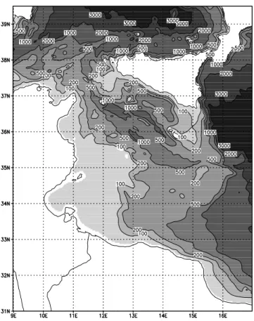
Fig. 1. SCRM domain and bathymetry obtained from U.S. Navy
DBDB1 by bilinear interpolation into the regional model grid. Depth in metres.
of sea surface in the Ligurian Sea was confined to the upper few metres of the sea and was associated with a period of weak winds.
Such changes in Sea Surface Temperature (SST) and re-lated changes in current speed and direction may affect other important physical and biological processes. In the Central Mediterranean the latter include the growth, concentration and retention of early life stages of fish populations (e.g. Brett, 1970; Bakun, 1996; Agostini and Bakun, 2002), the stock recruitment for important commercial species (Levi et al., 2003) and the reproductive strategies of small-pelagic species (Garc´ıa-Lafuente et al., 2005). In shelf seas (Ruardij et al., 1997) increases in stratification reduce vertical mixing and so limit nutrient supply and phytoplankton growth. Such effects are also believed to be very important in straits and channels where the current field is stronger and more com-plex and there is often higher biological production than in surrounding seas.
In this respect, the Central Mediterranean area studied here is important because of the channel flows and its role in link-ing the eastern and western Mediterranean sub-basins. The area is morphologically divided in two sub-areas, the Sar-dinia Channel to the west and the Sicily Channel to the east
(Fig. 1). The flows through the two channels are organ-ised in three main layers. The upper ocean flow is domi-nated by Modified Atlantic Water (MAW) driven primarily by the pressure gradient between the western and the east-ern basin. The flow is also strongly affected by wind forcing and bathymetry. Below this an intermediate layer, between about 200 and 500 m in the Sicily Channel, is dominated by the Levantine Intermediate Water (LIW) that flows from the eastern to western Mediterranean basin. The bottom layer contains the transitional Eastern Mediterranean Deep Water (tEMDW) which also flows westward underneath the LIW.
In the upper layer, the MAW flows east from the Strait of Gibraltar along the north African coast where it forms un-stable meanders that often create cyclonic and anticyclonic eddies with spatial scales of ∼200 km (Puillat et al., 2002). From the Sardinia Channel, two branches of MAW cross the Sicily Strait eastward. The first flows along the south-ern Sicily coast as an energetic meandering flow called the Atlantic Ionian Stream (AIS, e.g. Robinson et al., 1999; Warn-Varnas et al., 1999; Lermusiaux and Robinson, 2001). Strongest in summer, the AIS follows a complicated mean-dering path around three surface thermal features: the Ad-venture Bank Vortex, the Maltese Channel Crest and the Io-nian Shelf Break Vortex. The current brings nutrients into the surface layers and is ultimately responsible for the important little-pelagic-fish populations caught in this area (Garc´ıa-Lafuente et al., 2005). The interface between the fresh MAW of the AIS and the warmer Ionian Sea also produces the ther-mal filament known as the Maltese Front.
A second branch of MAW flows along the Tunisian coast as the Atlantic Tunisian Current (ATC) (Beranger et al., 2004). This is characterised by a high seasonal variability and a maximum volume transport in autumn (Manzella et al., 1988). In the summer the AIS, at its maximum intensity, bi-furcates southward at the trench past the Island of Pantelleria producing a weaker flow that also joins the ATC (Lermusiaux and Robinson, 2001).
In the present paper we report on the effects of the anoma-lous 2003 weather conditions on the surface and sub-surface temperatures and dynamics of the Central Mediterranean Sea simulated using a nested eddy resolving hydrodynamic 3-D model of the region. The model results are supported by remotely-sensed data and in situ observations made during the same period. Section 2 describes the model, the data used for validation and the methods used for analysis. Section 3 is concerned with the results from the study and covers at-mospheric forcing, the surface heat fluxes and model SSTs and changes in the model current field during the summer of 2003. Finally in Sect. 4 we summarize and discuss our findings.
2 Methods
A nested high resolution eddy resolving ocean circulation model was implemented and a 5-year hindcast simulation (2000–2004) was conducted in the Central Mediterranean area. The ocean responses to realistic atmospheric forcing from January 2000 to December 2004, have been analysed.
2.1 Model design
A new eddy resolving ocean model, the Sicily Channel Re-gional Model (SCRM), has been developed for the Sicily
Channel and surrounding areas. The model uses a
uni-form horizontal orthogonal grid with a resolution of 1/32◦
(∼3.5 km) in longitude and latitude (257×273 mesh points). In the vertical it uses 24 sigma levels (−1≤σ ≤0). The sigma levels are bottom following but follow a logarithmic distribu-tion near the surface. This permits more detail for the surface layer, while the other layers between bottom and surface are equally spaced. The high resolution SCRM should be ca-pable of resolving the mesoscale features, such as fronts and eddies, which have a horizontal scale characterised by the in-ternal Rossby deformation radius, ∼19 km (Manzella et al., 1988). The model grid is also sufficiently fine to resolve the important small scale bathymetric features in the region.
The model covers the area from 9◦E to 17◦E in longitude
and from 31◦N to 39.5◦N in latitude. Time integration is
done using a split explicit scheme in which the barotropic and baroclinic modes are integrated separately. The barotropic mode is integrated with a time step of 4 s and the baroclinic modes with a time step of 120 s.
The basic numerical formulation is based on the Princeton Ocean Model (POM), a three-dimensional primitive equation model (Blumberg and Mellor, 1987). POM timesteps equa-tions for the conservation temperature, salinity and horizon-tal momentum under the assumption that the ocean is incom-pressible, that it is in hydrostatic balance and that the Boussi-nesq approximation holds (Blumberg and Mellor, 1987). The equation of state used is an adaptation of the UNESCO equa-tion of state revised by Mellor (1991). The vertical mixing
coefficients KMfor momentum and KH for heat and salt are
calculated using the Mellor and Yamada (1982) turbulence
closure scheme, while the eddy viscosity coefficient AM is
calculated using the Smagorinsky (1993) parameterization.
The model bathymetry is based on the U.S. Navy 1/60◦
Digital Bathymetric Data Base (DBDB1) by bilinear inter-polation onto the SCRM grid. Additional light smoothing was applied to reduce the sigma coordinate pressure gradient error (Mellor et al., 1994). The resulting model bathymetry, as well as the model domain, is shown in Fig. 1. The max-imum depth is ∼3500 m, while the minmax-imum was set to be 5 m.
The model was initialised using data from the climatolog-ical run of Sorgente et al. (2003) and the model then inte-grated for the period 1 January 2000 to 31 December 2004.
During this period the model was forced using 6-hourly atmospheric analysis fields from the ECMWF. Although ECMWF re-analysis data would be more desirable this was not available for the period of interest. In order to avoid the presence of jumps due to changes in the analysis scheme, we checked the ECMWF documentation for major changes in their analysis system. On the basis of this check and the re-sults we obtain (see Sect. 3), we believe that there were no significant changes which affect the results presented here. A detailed description of parameterization of the surface boundary conditions can be found in Sorgente et al. (2003).
At its lateral open boundaries the model used oceano-graphic data from the OGCM-MFSPP large scale model of the Mediterranean (Pinardi and Masetti, 2000; Demirov and Pinardi, 2002). The large scale model uses a horizontal reso-lution of 1/8◦degrees and has 31 levels in the vertical. Data is interpolated from nearby grid points of the the large scale model to the open boundary points of the Sicily Channel Re-gional Model. In addition, to reduce the effect of interpola-tion errors, the total flux through each open boundary of the regional model is constrained to equal that through the same section of the large scale model. A detailed description of the nesting procedure is given in Pinardi et al. (2003) and Sorgente et al. (2003).
2.2 Satellite and hydrological data
The AVHRR SST data used in this analysis was derived from the 5-channel Advanced Very High Resolution Ra-diometers (AVHRR) on board of the NOAA −7, −9, −11,
−14, −16 and −17 polar orbiting satellites. Monthly
av-eraged data, derived from the ascending daytime pass on equal-angle grids of 8192 pixels/360 degrees, was obtained from the Physical Oceanography Distributed Active Archive Center (PO.DAAC) at the NASA Jet Propulsion Laboratory (http://podaac.jpl.nasa.gov). The data is normally referred to as the 4 km resolution data.
The CTD data was collected between the 11th and 21st July 2003 in the Sicily Channel area during oceanographic
cruise ANSIC03 of the N/V Urania. Hydrological data
(conductivity, temperature and depth) was acquired using a SBE911 plus CTD probe (Sea-Bird Inc.) with a 24 Niskin bottle rosette for water-column sampling. The data collected was quality-checked and processed following the MODB instructions (Brankart, 1994) using Seasoft software. The data was collected during four transects, T1, T2, T3 and T4 (Fig. 2) that cover the AIS area. The Section T1 runs from the south of Pantelleria Island to the western corner of Sicily, crossing the Adventure Bank, and contained 6 CTD stations. The Section T2 extends from just off Lampedusa Island to the Sicily Coast, with 11 CTD stations. T4 is located over the Ionic slope and has a NE direction toward the Ionian shelf break, with 4 CTD stations. These three transects lie at right angles to the southern coast of Sicily. The final tran-sect T3, with 15 CTD stations, is parallel to the coast. At all
12oE 13oE 14oE 15oE 16oE 35oN 36oN 37oN 38oN T1 T2 T3 T4
Fig. 2. CTD sampling points collected during 11–21 July 2003
pe-riod. They are organized in 4 transect (T1 to T4) covering the AIS area.
the stations the shallowest data collected was from a depth of 5 m. To make a direct comparison between the SCRM and observations, model profiles were extracted which matched the CTD sampling points in time (day) and space (±3.5 km).
2.3 Wavelet analysis
Two-dimensional fields of variables from either the ECMWF atmospheric input or the SCRM output were averaged in a two-step process. First they were averaged over the whole SCRM domain and then they were averaged in time to pro-duce a time series of daily spatial averages. Monthly aver-ages were also calculated for the whole 5-year period. We then removed seasonal effects by subtracting the 5-year av-erage monthly values from the daily time series and normal-izing the results by the monthly standard deviation:
xn=
x − xm
σm
, (1)
where x is the daily data value, xm is the climatological
(2000–2004) monthly mean for a corresponding month and
σm is the related monthly standard deviation. A similar
scheme was applied to the satellite monthly time series of SST. The resulting time series were then analysed further using Fourier Transforms (FT) and the Continuous Wavelet Transforms (CWT).
The CWT is useful for analysing time series data with a strong non-stationary component. This is because it allows localization of energetic events in both time, using transla-tions of the mother wavelet defined below, and in frequency, using wavelets of different dilation. In contrast the FT is only able to recognise the location and magnitude of a signal
in the frequency domain. However the FT remains very ap-propriate for the analysis of stationary data, which does not require time localization information or to get an overview of the main components of a signal, as in our analysis.
Before performing the CWT and the FT we removed trends from the data to reduce spurious low frequency sig-nals. By definition, a mother wavelet is a function with a zero mean and must be defined in both time and frequency dimensions. To calculate the CWT we have chosen the Mor-let waveMor-let as the mother waveMor-let, which is very useful for oceanographic data both in its real or complex forms (Tor-rence and Compo, 1998; Massel, 2001; Cromwell, 2001).
As in Torrence and Compo (1998) we define the Contin-uous Wavelet Transform as the convolution of our discrete time series, constituted by the xnelements, with dilations and translations of the mother wavelet function.
The wavelet plots, which show wavelet as a function of time and period, also show the 95% significance level con-tours as thick black lines. These significant levels were esti-mated by comparing the wavelet spectrum with a red-noise signal (commonly used for geophysical time series), com-puted on the basis of the lag-1 autocorrelation of the same time series. The wavelet plots also show the Cone Of Influ-ence (COI), a triangular region in which the wavelet results are not affected by the beginning or end of the time series.
3 Results
In this section the results of the wavelet analyses of the at-mospheric variables and surface heat fluxes (Sect. 3.1) are presented first, to give an overview of surface atmospheric forcing producing the anomalous warming of sea surface. Then the spectral analyses of the simulated and remotely-sensed SST (Sect. 3.2) are discussed. The most noticeable monthly values for each parameter and, when necessary, the seasonal and/or interannual trends are presented. The paral-lel observation of the time-frequency (wavelet and FT plots) data and of the raw time series (daily and monthly averaged) gives a complete picture of the variability of the analysed variables. The comparison between simulated and remotely-sensed SST anomalies maps shows the ability of the model to reproduce the spatial variability of the observed event. Sec-tion 3.2 contains observaSec-tions of water stratificaSec-tion and sur-face and sub-sursur-face currents modifications during the sum-mer of 2003. A comparison with in situ CTD data is per-formed to confirm the agreement of SCRM results with the measurements during the heat wave event, and more in gen-eral the ability of the model to reproduce the sub-surface hy-drographic features.
3.1 Surface forcing and heat fluxes
In the summer of 2003 the air temperature at 2 m reached
2000.5 2001 2001.5 2002 2002.5 2003 2003.5 2004 2004.5 −2 0 2 4 (a)
Fourier period (days)
Years (b) 2000.5 2001 2001.5 2002 2002.5 2003 2003.5 2004 2004.5 0 100 200 300 400 500 600 5 10 15 x 104 0 100 200 300 400 500 600 Power (c)
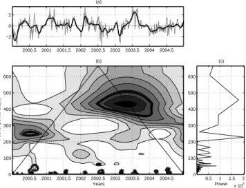
Fig. 3. Air temperature. (a) anomalies daily (thin gray line) and
monthly (thick black line) time series normalized by standard devi-ation; (b) anomalies CWT spectrum; (c) FT Periodogram. In sub-plot (b) we can see two different important anomalies: the first is a low frequency anomaly and the second, temporarily superimposed to the first, with a higher frequency (250 days); both are centred in the year 2003. The highest spectrum magnitude is reached in cor-respondence with the higher frequency 2003 anomaly that extends from autumn 2002 to autumn 2003, then including the low values of winter 2003. In the wavelet plot, the 95% significance level con-tours (thick black line) and the area known as Cone Of Influence (COI, the thin black line that forms a triangular area) that delimits the zone of the plot in without edge effects (inside the triangle), are also drawn.
parts of Europe. This high temperature was mainly caused by the prevalence of anticyclonic conditions (Black et al., 2004). Furthermore, the JJA monthly means of air temperature over
central Europe reached values up to ∼5◦C warmer than in
the last 150 years climatology. Over a larger European area,
values have been recorded as ∼3◦C warmer compared to the
period 1961–1990 (Sch¨ar et al., 2004).
From our analyses, in respect to the 2000–2004 clima-tology, in the 2003 JJA months, the daily anomalies time series of air temperature (at 2 m) over the SCRM domain reached the highest values of the entire period (up to 3–4◦C). In Fig. 3 the normalized anomalies time series, the wavelet spectrum and the periodogram (Fourier spectrum) relative to this parameter are shown, respectively. The presence of two distinct anomalies at two distinct frequencies (Fourier period of ∼450 and ∼220 days) are observed, temporally superim-posed and centred in the year 2003. We observe that both the signals reach their maximum magnitude in a time period situated between January/February (JF) 2003, when the cold-est anomaly of the whole period is recorded, and the warm anomaly of the summer 2003. We may also notice a reduc-tion of the high frequency signal, mainly due to the persis-tence of anticyclonic conditions, whose effect is in fact
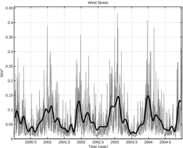
re-2000.5 2001 2001.5 2002 2002.5 2003 2003.5 2004 2004.5 0 0.05 0.1 0.15 0.2 0.25 0.3 0.35 0.4 0.45 Wind Stress N/m 2 Time (year)
Fig. 4. Wind stress daily (thin gray line) and monthly (thick black
line) time series, characterized by a high frequency variability. The two absolute maxima of monthly averaged wind stress intensity are in February and December 2003 and the absolute minimum in June, July and August of the same year.
ducing the short term variability. Another weak, but statisti-cally significant signal, at a shorter Fourier period (120 days), is consistent with anomalous negative values of air tempera-ture in December 2001/January 2002.
The wind stress time series, computed from the ECMWF atmospheric fields and used as forcing at the surface is shown in Fig. 4. The highest monthly values of wind stress are reached in February and December 2003 (respectively
0.16×10⁻² and 0.15×10⁻²Nm−2), while the lowest are
reached in the summer months of the same year. This last value is consistent with the computed high values of air and sea surface temperature (see below) for this period.
The spectral analyses performed on the anomalies series for the wind stress intensity (Fig. 5) show that a great part of non-seasonal variability is concentrated at the highest fre-quencies, with the great exception of the very low frequency signal temporally coincident with the air temperature anoma-lies of 2003, although it was partially outside of the COI.
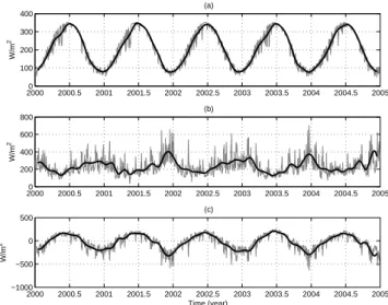
The daily and monthly averaged time series of solar radi-ation, upward heat flux (i.e. the sum of the latent heat flux Qe, longwave radiation Qband sensible hear flux Qh), and net heat flux are shown in Fig. 6.
The solar radiation time series (Fig. 6a) shows a strong seasonal variability. In performing the wavelet analysis, no significant anomaly was found with the exception of a weak signal at the beginning of 2003 (not shown). The upward heat flux (Fig. 6b) appeared to have a more complicated struc-ture compared to the solar radiation, due to its dependence on wind intensity and air temperature. The upward fluxes
2000.5 2001 2001.5 2002 2002.5 2003 2003.5 2004 2004.5 0
2 4
(a)
Fourier period (days)
Years (b) 2000.5 2001 2001.5 2002 2002.5 2003 2003.5 2004 2004.5 0 100 200 300 400 500 600 0.5 1 1.5 2 x 10⁴ 0 100 200 300 400 500 600 Power (c)
Fig. 5. Wind stress. (a) anomalies daily (thin gray line) and monthly
(thick black line) time series normalized by standard deviation; (b) anomalies CWT spectrum; (c) FT Periodogram. In subplot (b) note that the main magnitude is reached at the highest frequencies with the an exception of the strong interannual signal centred in 2003.
20000 2000.5 2001 2001.5 2002 2002.5 2003 2003.5 2004 2004.5 2005 100 200 300 400 (a) W/m 2 20000 2000.5 2001 2001.5 2002 2002.5 2003 2003.5 2004 2004.5 2005 200 400 600 800 W/m 2 (b) 2000 2000.5 2001 2001.5 2002 2002.5 2003 2003.5 2004 2004.5 2005 −1000 −500 0 500 W/m 2 (c) Time (year)
Fig. 6. Surface Heat fluxes. (a) Daily (thin gray line) and monthly
(thick black line) Solar Radiation; (b) Daily and monthly Heat Loss, i.e. the sum of Qe, Qband Qh; (c) Daily and monthly Net Heat flux
(Solar Radiation-Heat Loss).
respect to the 5-year climatology, we calculated the strongest positive monthly anomalies in February 2003 (+1.54, dimen-sionless). They were calculated by subtracting the monthly mean from the monthly climatological value and then nor-malising by standard deviation, in a similar way as for the daily anomalies time series. The strongest negative (−1.62 and −1.63) monthly anomalies were in March 2001 and June 2003. A strong decrease of fluxes in comparison to the 5-year
2000.5 2001 2001.5 2002 2002.5 2003 2003.5 2004 2004.5 −2 0 2 4 (a)
Fourier period (days)
Years (b) 2000.5 2001 2001.5 2002 2002.5 2003 2003.5 2004 2004.5 0 100 200 300 400 500 600 1 2 3 4 x 10⁴ 0 100 200 300 400 500 600 Power (c)
Fig. 7. Upward Heat flux. (a) anomalies daily (thin gray line) and
monthly (thick black line) time series normalized by standard devia-tion; (b) anomalies CWT spectrum; (c) FT Periodogram. The main anomaly is in the summer 2003. The rest of the signal is mainly located at the highest frequencies.
climatology was also noticeable from the months of April to November 2003, with the absolute minima in JJA.
A strong interannual variability on a monthly basis, as well as a moderate variability on annual basis is therefore intu-itive, but no conclusion can be drawn on the frequencies and periods of these deviations when considering only the aver-aged values. The analysis of the spectra of the anomalies time series (wavelet and Fourier spectra) provides this infor-mation. In Fig. 7 the daily anomalies time series (normalized by standard deviation) of upward fluxes and the spectral anal-yses of data are shown.
The two spectra of Figs. 7b and c indicate the presence of a significant low frequency signal in the anomalies time series with a Fourier period of ∼450–500 days. This sig-nal coincided with a strong increase of upward fluxes in the winter and spring 2003, and their decrease in summer 2003. This low frequency signal had a very good agreement with other sea surface and atmospheric anomalies we registered in the same time-frequency location (see below), although it is located just out of the COI. The residual variability of the anomalies time series is related mainly to the high frequency atmospheric variability.
In Fig. 8 the monthly time series of the three components of upward flux was compared. The main component is the la-tent heat flux (Qe), followed by the longwave radiation (Qb), while the sensible heat (Qh) is the smallest in terms of total budget.
The latent heat flux reached its maximum seasonal val-ues in the autumn and winter months (remember that for the Qe, Qband Qhterms, positive values indicated a flux from the sea surface to the atmosphere). The absolute maximum
2000 2000.5 2001 2001.5 2002 2002.5 2003 2003.5 2004 2004.5 2005 −50 0 50 100 150 200 250 W/m 2 Time (year)
Fig. 8. Upward heat flux components monthly time series. Latent
heat (Qe, black solid line); Longwave radiation (Qb, black dashed
line); Sensible heat (Qh, gray solid line).
was reached in November and December 2001 with 222 and
225 W m−2respectively, while the minimum was reached in
June 2003 with 48 W m−2. This last minimum corresponds
to the major anomaly observed for the total upward heat
fluxes. Also the Qband Qh fluxes had their seasonal
max-ima in the autumn and winter months. Very low 3-month av-eraged values have been reached for both fluxes in JJA 2003 with ∼80 W m−2and ∼1 W m−2, respectively.
The net heat flux values (Fig. 6c), 5-year averaged, are positive (i.e. the sea gain heat) in the months from April
to August, with a maximum value of +166 W m−2in June.
Values are negative in the other months with a minimum of
−251 W m−2 in December. The behaviour of the net heat
flux as well as its non seasonal variability, is driven by the upward heat flux, considering the very low interannual vari-ability of the solar radiation term. The wavelet spectrum for the net heat flux anomalies (not shown) is almost equal to the upward flux. In JJA 2003 we calculated the highest posi-tive anomaly of net heat fluxes (1.54 for June–July and 1.58 for August, dimensionless), which indicate a very strong heat gain.
3.2 Sea Surface Temperature and dynamical response
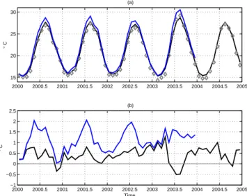
The SST monthly time series (Fig. 9a) simulated by the model shows a strong annual cycle and a somewhat weaker interannual signal, mainly related to the strong heat gain dur-ing the summer 2003.
In order to compare the simulated SST (temperatures are interpolated from sigma levels to the depth of 0.5 m) to real observed values, the means computed from satellite SST monthly data have been compared with the SST time series
2000 2000.5 2001 2001.5 2002 2002.5 2003 2003.5 2004 2004.5 2005 15 20 25 30 (a) ° C 2000 2000.5 2001 2001.5 2002 2002.5 2003 2003.5 2004 2004.5 2005 −1 −0.5 0 0.5 1 1.5 2 2.5 (b) ° C Time
Fig. 9. SST. (a) SST monthly time series (averaged on the entire
do-main) calculated with and without the relaxation term (black curve and blue curve respectively) and extrapolated from satellite data (grey diamonds); (b) Difference between the model SST and satel-lite SST. The black curve shows the difference in the case of a model setup with the relaxation term; the blue curve is the case without relaxation. With the relaxation scheme, the SCRM SST shows a better fit with the remotely-sensed SST. The difference ranges from
−0.5◦C to 1.3◦C, reaching both the highest and lowest values dur-ing the 2003 heatwave.
simulated from the SCRM, both in terms of monthly means and the wavelet spectra.
The computed domain-averaged SST in Fig. 9a (black curve) is in a good agreement with the satellite monthly data (gray diamonds), with an average offset between the two
se-ries of ∼+0.4◦C. The difference between the two time
se-ries, shown in Fig. 9b (black curve), ranges from −0.5◦C to
1.3◦C, reaching the highest and lowest values in agreement
with the surface anomalies of 2003. The satellite monthly means are generally colder than the model output, with the exception of the summer 2003 when the model underesti-mated the real SST temperature, assuming no error for the remotely-sensed data. The underestimated SST in summer 2003 is due to a correction term in the heat flux calculations, which generates a smoothing effect for the upward fluxes. This is confirmed by a second numerical simulation with-out any relaxation to the climatology fields (Figs. 9a, b, blue curves), which shows a larger overestimation of temperatures
(averaged values of about +1.1◦C) along the entire
simula-tion period and also during summer 2003. So, the employ-ment of the relaxation term is an efficient means to reduce the bias with respect to observations, and the chosen level of re-laxation is a good compromise to reproduce the normal years and the extreme event sufficiently well. To quantify the cor-rection in terms of net heat fluxes, we observed that the mean
2000.5 2001 2001.5 2002 2002.5 2003 2003.5 2004 2004.5 −2
0 2
(a)
Fourier period (days)
Years (b) 2000.5 2001 2001.5 2002 2002.5 2003 2003.5 2004 2004.5 0 100 200 300 400 500 600 0.5 1 1.5 2 x 10⁵ 0 100 200 300 400 500 600 Power (c)
Fig. 10. Modelled SST. (a) anomalies daily (thin gray line) and
monthly (thick black line) time series normalized by standard de-viation; (b) anomalies CWT spectrum; (c) FT Periodogram. The wavelet analysis of the SST anomalies shows a main anomalous long-wave signal that coincides with the 2003 summer heat wave.
daily correction is ∼–12 W m−2with a standard deviation of
∼14 W m−2. The relaxation acts mainly in the summer
pe-riods increasing the heat lost by the sea, and less during the winter time.
The spectral analysis of SST anomalies daily time series (Fig. 10) shows a main anomaly with a Fourier period of
∼450 days, which is consistent with the heatwave affecting
Europe and the Mediterranean area during the summer 2003. Although it cuts off the boundary of the COI, this wave has a level of significance greater than 95%. Another weak signal, related to a negative anomaly, is detected at the beginning of the time series, but it was not considered since it is entirely out of the COI and has a low significance level.
It is interesting to observe that the main wavelet signal was not limited to summer 2003. With a 95% significance level (thick black line) it extended from the middle of 2002 to the beginning of 2004, covering more than a 1.5 year inter-val. Furthermore, by considering only the highest magnitude of the spectrum, the main wavelet signal was reached be-tween December 2002 and August 2003, including also the strong heat loss in winter 2003 (see also the wind stress and the upward heat fluxes spectra) and the heatwave of sum-mer 2003. The presence of statistically significant signals at high frequencies during the entire series, although they register very low power spectra, was due to the related high frequency variability of wind stress and to very high auto-correlation (lag-1 autoauto-correlation >0.95) of the SST time se-ries. Despite the weakly underestimated SST in the period of the heatwave, the spectral analysis of SST monthly time series of the anomalies (Fig. 11) obtained from satellite mea-surements, reveals a wavelet spectrum almost equal, in the
2000.5 2001 2001.5 2002 2002.5 2003 2003.5 2004 2004.5 2005 −1
0 1
(a)
Fourier period (days)
Years (b) 2000.5 2001 2001.5 2002 2002.5 2003 2003.5 2004 2004.5 2005 0 100 200 300 400 500 600 100 200 300 0 100 200 300 400 500 600 Power (c)
Fig. 11. Satellite SST. (a) anomalies monthly time series
normal-ized by standard deviation; (b) anomalies CWT spectrum; (c) FT Periodogram. The wavelet analysis of the SST anomalies from satellite is consistent with the spectrum derived from the model out-put. The heatwave event is located in the same time-frequency re-gion.
lower frequencies, to the spectrum obtained from the anal-ysis of the simulated SST time series (compare Fig. 10 and Fig. 11). Both the location in time and the Fourier period of the anomaly are well simulated by the model.
The monthly SST anomaly fields computed from the remotely-sensed data and simulated by SCRM during June 2003, (the highest anomalies of JJA 2003 period) are shown in Fig. 12. The measured anomalies (Fig. 12, left panel) are slightly higher than those simulated by the model (Fig. 12, right panel), about 0.4◦C basin averaged, although the spa-tial distribution is very similar. The satellite anomalies are located mainly in the south Tyrrhenian Sea with values above
2.4◦C, while in the Sicily Channel they range from 1.2 to
2.1◦C, and generally decrease moving southward. A
simi-lar horizontal distribution of anomalies is reproduced by the model simulation, but over the Sicily channel the range is
rather limited, with values from 0.6 to 1.2◦C. In terms of
absolute values, the highest temperatures occurred in August 2003 with values over 29.5◦C in the Tyrrhenian Sea and east-ward of Sicily Coast, while over the Tunisian Shelf the SST reached about 31◦C (not shown).
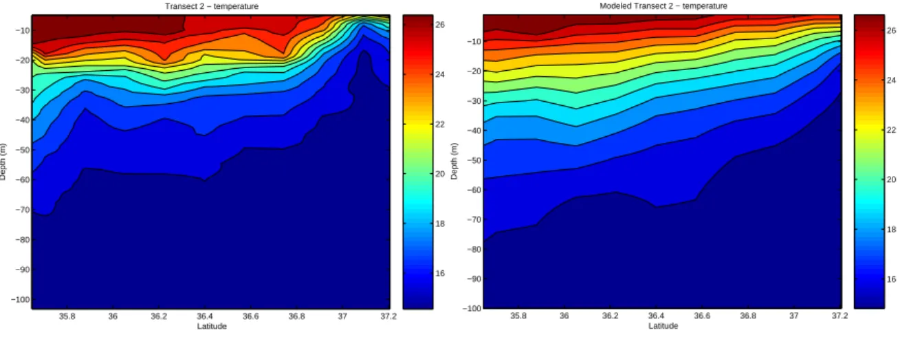
The combined effect of the sea surface warming and the low wind intensity over the upper layers is shown in Fig. 13, referring to the measurements collected along the T2 tran-sect. The temperature measurements along this section show a water column characterized by a strong vertical stratifica-tion, with SST values ranging from 26◦C (offshore) to 22◦C (closer to the south coast of Sicily). The upper layer is char-acterized by a thin mixed layer, between the surface and
Fig. 12. Monthly SST anomaly fields for the remotely-sensed (left) and simulated by SCRM (right) for June 2003. The anomalies are referred
respectively to the satellite and model minus climatology, where the climatology represents monthly averages for the period 2001–2004.
Transect 2 − temperature Latitude Depth (m) 35.8 36 36.2 36.4 36.6 36.8 37 37.2 −100 −90 −80 −70 −60 −50 −40 −30 −20 −10 16 18 20 22 24 26
Modeled Transect 2 − temperature
Latitude Depth (m) 35.8 36 36.2 36.4 36.6 36.8 37 37.2 −100 −90 −80 −70 −60 −50 −40 −30 −20 −10 16 18 20 22 24 26
Fig. 13. Vertical cross section of temperature along the T2 transect: Measurements (left) and simulation (right). Units are◦C.
pronounced thermocline is located at ∼25 m depth, reach-ing the surface near the southern coast of Sicily, at about 50 km offshore. The related simulated temperature section (Fig. 13, right panel), shows the same temperature range with the isotherms sloped towards the surface, that would indi-cate the presence of coastal upwelling, induced by the
north-westerly wind and by the inertia of the isopycnals dome of the AIS meanders. Due to the advection scheme, SCRM tends to underestimate the mixed layer thickness, with high-est temperature differences in the thermocline layer, where the model is warmer in respect to the observations.
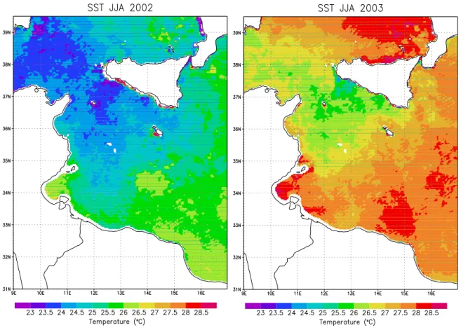
Fig. 14. Remotely-sensed Sea Surface Temperature averaged for JJA 2002 (left) and 2003 (right).
.
A comparison of the sea surface temperature observed by satellite, averaged for JJA 2002 and 2003, shown in Fig. 14, illustrates the exceptionally high SST recorded in the Sicily Channel during the summer of 2003. The surface water
tem-perature was found up to ∼3◦C degrees warmer than the
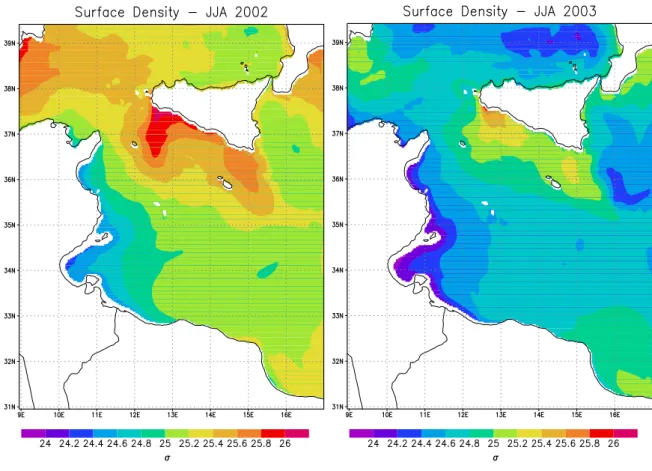
previous year, with a sensible decrease of the surface den-sity (Fig. 15, right panel) with respect to 2002 (Fig. 15, left panel). This effect only dissipated in autumn, with an on-set of cold and strong winds. The decrease of superficial density, observed over the whole domain, mainly affected its western part, determining a decrease of the usual west-east density gradient, having large implications on eastward flow of MAW through the Sicily Channel. In fact, as discussed by Molcard et al. (2002), the increase/decrease of the west-east density gradient play a key role in modulating the intensity of the AIS flow. Particularly this study shows that the AIS flow is enhanced when this gradient increases, to the detriment of the ATC, and vice-versa.
The simulated velocity fields over the AIS area (Fig. 16) show the AIS reduced in intensity, because of the previously seen reduction of density gradient and decrease of westerly winds. Together they are responsible for the generation and modulation of the velocity field. Current velocities of the
AIS simulated by the SCRM in JJA 2003 are of the order of
∼0.2–0.3 ms−1(compared to ∼0.3–0.4 ms−1of 2002) over
the Adventure Bank, with modifications in the path of the AIS along it. Usually the AIS path starts at the Sicily Strait as an energetic and well developed meander, controlled by bathymetry, over the Adventure Bank (Fig. 16, left) char-acterized by noticeable cool water, clearly visible also by satellite images (Fig. 14, left panel). In JJA 2003, the AIS appears less winding, weaker and shifted towards the Sicily coast (Fig. 16, right). The horizontal extension of the Ad-venture Bank Vortex appears rather limited, with a reduc-tion of the off-shore upwelling extension and mixing, as ob-served also by the SST images (Fig. 14, right panel) and from the CTD data along the Section T1 (Fig. 17, left). The salinity minimum (Fig. 17, right) depicts the position of the AIS core, characterized by a density front (not shown) to the
left of the current, which extends to ∼37.2◦N. Because the
MAW associated to the AIS flow moves south of the density front, the MAW flow tends to be more flattened along the southern Sicily coast. Due to this unusual path of the AIS, modifications of the coastal upwelling south of Sicily are also observed. In fact the offshore spread of the upwelling is controlled by AIS flow and its variability. Generally the
Fig. 15. Simulated sea surface density averaged for JJA 2002 (left) and 2003 year (right). Units are in σ density (kg m−3).
Fig. 16. The total velocity field at 30 m depth averaged for JJA 2002 and 2003, respectively. The domain is reduced over the AIS area. The
AIS in the year 2003 has a reduced meandering behaviour, while the ATC has an increased intensity.
upwelling area extends for a considerable distance offshore, about 100 km, especially over the Adventure bank forced by the cyclonic Adventure Bank Vortex and over the Malta
shelf, forced by Malta Channel Crest (Garc´ıa-Lafuente et al.,
2002). During JJA 2003 the upwelling area appears
Transect 1 − temperature Latitude Depth (m) 36.7 36.8 36.9 37 37.1 37.2 37.3 37.4 −100 −90 −80 −70 −60 −50 −40 −30 −20 −10 16 18 20 22 24 26 Transect 1 − salinity Latitude Depth (m) 36.7 36.8 36.9 37 37.1 37.2 37.3 37.4 −100 −90 −80 −70 −60 −50 −40 −30 −20 −10 37.4 37.6 37.8 38 38.2 38.4 38.6
Fig. 17. Observed temperature (left) and salinity (right) fields along the T1 transect during the Ansic2003 cruise. Units are◦C and psu, respectively.
Fig. 18. Simulated temperature at 30 m depth (left) and at the surface (right), averaged over the period JJA 2003.
modified path of AIS. The summer coastal upwelling and the southeastward advection of cold patches is well simulated by the SCRM in the form of long plumes and filaments running along the whole southern coast of Sicily. At 30 m depth, the temperatures range approximately from 16◦C to 19◦C in the
Sicilian shelf, and from 20◦C to 22◦C in the offshore area. At the surface, the upwelling area disappears almost completely (see right panels of Figs. 18 and 14), hidden by the superfi-cial layer of warm waters that block the upwelling of deep and cold water to the surface.
Transect 4 − temperature Latitude Depth (m) 36.05 36.1 36.15 36.2 36.25 36.3 36.35 36.4 36.45 36.5 −60 −50 −40 −30 −20 −10 16 18 20 22 24 26 Transect 4 − salinity Latitude Depth (m) 36.05 36.1 36.15 36.2 36.25 36.3 36.35 36.4 36.45 36.5 −60 −50 −40 −30 −20 −10 37.8 37.9 38 38.1 38.2 38.3 38.4 38.5 38.6 38.7
Fig. 19. Observed temperature (left) and salinity (right) fields along the T4 transect during the Ansic2003 cruise. Units are◦C and psu, respectively.
The AIS proceeds south-eastward and loops back to the north of Malta forming the Maltese Channel Anticyclone, south-east of the Maltese Channel Crest (Fig. 16). In or-der to maintain the alongshore geostrophic current, the un-derlying LIW ascends toward the surface (Garc´ıa-Lafuente et al., 2002). As reported also by Piccioni et al. (1988), the signature of this mechanism is represented by the constant presence of colder and saltier water masses along the Sicil-ian coast. During the JJA 2003 the LIW rises up to about 20 m depth, overlapped by the warm upper layer, a feature confirmed also by measurements along the T3 transect (not shown).
As the AIS reaches the sharp shelf break (north-east of Malta), it forms a weak cyclonic vortex (the Ionian Shelf Break vortex) and proceeds directly eastward into the Io-nian Sea (Fig. 16), without turning northward. It flows along the bathymetry before plunging into the Ionian basin. The absence of the northward extension of the AIS (NAIS) at the Ionian Shelf Break (Robinson et al., 1999; Warn-Varnas et al., 1999; Lermusiaux and Robinson, 2001; Beranger et al., 2004), confirmed its intermittent nature, which seems to be driven by the surface circulation off the eastern coast of Sicily and by the density gradient (Molcard et al., 2002) be-tween Sicily Channel and Ionian waters. The salinity dis-tribution along the Section T4 (Fig. 19) can not confirm the presence of NAIS, due to its limited horizontal extension, but it suggests the core of MAW, slightly fresher (the difference is about 0.05 psu) and deeper in respect to the model,
out-flowing from the channel at 36◦N and about 20 m depth.
To the contrary of the weakened AIS during the JJA 2003, the SCRM shows the MAW flow associated with the ATC reinforced (Fig. 16, right), while ATC is generally weak or not observed during the summer months (Robinson et al., 1999; Beranger et al., 2004). This current moves eastward, close to the African shelf edge, as a coastal current mainly
along the 200 m isobath, reaching values of 2.0 ms−1. The
MAW core transported by ATC is identified in the verti-cal distribution of salinity observed along T2 (left panel of Fig. 20), by an unusually low values near the Lampedusa Is-land (∼37 psu at ∼30 m depth, close to the southern bound-ary of T2). In this region the model depicts features similar to the observed ones, with an almost equal location of AIS and ATC flows (Fig. 20, right panel). Low salinity values of ATC could be related to the reduced impact of wind stress on the MAW/LIW mixing during the JJA 2003. In fact, although SCRM overestimates the minimum of salinity (37.4 psu at 30 m, compare the two panels of Fig. 20) and although the MAW inflow through the Sicily Strait is weaker during the summer time (Manzella, 1994; Sorgente et al., 2003), the model simulates a larger southward spreading of the mini-mum of salinity along the ATC in summer 2003 (not shown). The ATC increase, shown in Fig. 16 and supported by the observation of very low salinity values near Lampedusa, may be related to the reduction of the AIS flow, in turn due to the decrease of the west-east density gradient and to the weak-ened westerly winds. As mentioned above, the mechanism of compensation of ATC/AIS flows, mainly due to variations of the density gradient, was observed also in the study of Molcard et al. (2002).
The comparison of simulated and measured profiles of salinity suggests the main difference is related to the range of salinity. The variability of the simulated salinity is smaller due to the overestimated minimum in the model. However, the main water masses crossing the area (MAW and LIW) seem to be well reproduced by the model. In order to quan-tify the observed gap between the two datasets we calcu-lated the Root Mean Squared Error (RMSE) between sim-ulated and measured temperature and salinity for each pro-file. The RMSE has been computed using the CTD values at depths matching the model sigma levels. The RMSEs of
Transect 2 − salinity Latitude Depth (m) 35.8 36 36.2 36.4 36.6 36.8 37 37.2 −100 −90 −80 −70 −60 −50 −40 −30 −20 −10 37 37.2 37.4 37.6 37.8 38 38.2
Modeled Transect 2 − salinity
Latitude Depth (m) 35.8 36 36.2 36.4 36.6 36.8 37 37.2 −100 −90 −80 −70 −60 −50 −40 −30 −20 −10 37 37.2 37.4 37.6 37.8 38 38.2
Fig. 20. Salinity vertical section along the T2 transect: Measurements (left) and simulation (right). Units are psu.
Fig. 21. Horizonal distribution of salinity RMSE between measured
and modelled profiles. The profile over the Adventure Bank shows the worst agreement.
temperature profiles range from 0.2◦C to 2.2◦C with an av-erage of 0.9◦C, while the range for salinity is from 0.1 psu to 0.6 psu, with the average value of 0.2 psu. In order to assess the spatial variability of the salinity RMSE, a map was obtained by horizontally interpolating the depth aver-aged RMSE values from each CTD station (Fig. 21). From the salinity RMSE map (the distribution of RMSEs of tem-peratures is substantially equal) we may immediately see the central profile of T1, collected over the Adventure Bank (SW corner of Sicily), has the lower agreement with the measure-ments, while the other analysed profiles show quite a good estimation of salinity and temperature. The disagreement of this T1 profile might be related to small differences (between model and observations) in the location of the Adventure
Bank Vortex, forcing the AIS to flow more or less close to the coast. It is not trivial to compare measured data with the sim-ulated values because the temporal and spatial coordinates do not necessarily match exactly. The locally highly vari-able and complex bathymetry of the Sicily Channel can have large variations on depth for a small horizontal displacement. This means that a “point-to-point” comparison, attempted in this section, may be easily affected by error due to inexact matching of data. This mismatching problem negatively af-fects the “bad profile” of T1, because it is located just at the boundary between the shelf and the continental slope, inside an area of large bathymetric variability. In fact, in this case, the simulated and measured profiles show large differences in depth.
4 Conclusions
During the summer of 2003 in many parts of Europe, surface air temperatures reached the highest values recorded over the last 150 years. Here we have shown that in the Central Mediterranean region, the summer 2003 temperatures at sea were also the highest during the five year study period.
Wavelet analysis of air temperatures show that, during the study period, air temperatures over the sea were dominated by two low frequency events. These both peaked in the sum-mer of 2003 but had separate periods. A similar analysis of the wind stress shows that the variability was dominated by high frequencies but that there was also a low frequency peak centred in 2003, consistent with the heating anomaly but largely outside of the wavelet COI. This peak was asso-ciated with the low wind stress values observed during the summer of 2003 and also with the higher values of wind stress observed during in the winters of 2003 and 2004.
These anomalies of the air temperature and winds caused significant changes in the heat fluxes over the study re-gion. We find that at low frequencies the upward flux was
determined primarily by the air temperature and partially by the wind stress, while at high frequencies the flux was deter-mined more by the wind stress variability. We also find that the interannual variability of the total heat fluxes was deter-mined primarily by the upward fluxes because of the small changes in the seasonality and periodicity of the downward heat transport (primarily solar radiation). All three compo-nents of the upward fluxes (evaporation, longwave radiation and sensible heat) were involved in the anomalies of 2003. However, the latent heat flux had the main effect as it showed the maximum decrease during the period.
The analyses of other atmospheric parameters that might be involved (e.g. the cloud cover and the relative humidity) did not show any peaks connected with the heatwave. As there were no significant anomalies in the relative humidity during the summer of 2003, the increased air temperature means that the absolute humidity must also have increased. The difference between the saturated absolute humidity at the sea surface and the air humidity was therefore reduced, pos-sibly explaining the strong decrease of observed latent heat flux.
The SST anomalies observed in the model in the Sicily Strait seem to be related to both the air temperature and the wind stress intensity. The atmospheric anomalies that Sutton et al. (2004) relates to very large-scale atmospheric forcing like the AMO, are correlated at regional scale with the sur-face heat upward fluxes, which show their consistency with the low frequency signal of the heatwave. Furthermore, the spectral analyses show that this long period signal is not time wise limited to the summer months of 2003, but it is a part of a longer lasting anomaly from autumn 2002 to winter 2003, in agreement with negative anomalies of SST values and pos-itive anomalies of upward fluxes also. The Fourier period of this signal suggests that the anomaly must have covered a larger time window than only the few summer months of 2003.
The model SST calculated during the 5-year run agrees well with the AVHRR data but shows a positive bias of
+0.4◦C (i.e. the model values are a little warmer than the
satellite data). The difference turns out to be greater in cor-respondence with extreme values, either positive or negative. This should be due to the presence of the relaxation term in the computation of upward fluxes, but the term is needed for a realistic SST estimates, as demonstrated in the second experiment in which we removed the nudging term, conse-quently obtaining worse results. However, as observed in the comparison between SST wavelet spectra obtained by satellite measurements and by model results, the effects of the 2003 European heatwave on the sea surface are well de-scribed and defined in the time-frequency domain. Addition-ally, the analysis of the spatial distribution of the anomalies show the overheating affected mainly the NW part of our do-main, in agreement with satellite observations. In fact the atmospheric anomalies of summer 2003, as described in lit-erature (e.g. Black et al., 2004; Marullo et al., 2003),
per-sisted mainly in western Europe and the western Mediter-ranean area.
The same atmospheric forcing responsible for the heat fluxes and SST anomalies are probably also responsible for the modified AIS and ATC flows observed in the same pe-riod and for the reduced offshore extension of the upwelling and the stronger stratification found along the southern Sicily coast.
The AIS showed a reduced meandering behaviour and a decreased intensity during the period of the anomaly. In con-trast the ATC appeared enhanced, mainly forced by changes in the longitudinal density gradient. The changes in the two currents may be related. Their flow is indeed out of phase: when the AIS starts to decrease (autumn) the ATC increases (Manzella et al., 1988), and vice-versa, as they transport wa-ter masses (MAW) originating as two branches of the same current. So, in order to conserve the mass transport they have to modulate their flow. In fact during the 2003 summer the AIS decreased its intensity mainly due to the diminished hor-izontal density gradient and to the observed drastic reduction of westerly winds, in turn reducing its meandering and de-creasing of the off-shore extension of upwelling, that nor-mally positively feeds back with the AIS. In this scenario of a weaker AIS, the MAW, despite the probable reduction of its total flow crossing the Sicily Channel due to the diminished density gradient (Molcard et al., 2002), has to find a “new” summer path to cross the Channel: it is transported mainly by the increased ATC in that period. This hypothesis will be an object of further investigations.
The observations of the sub-surface features have been supported by CTD data, which also assessed the good skill of the model to reproduce the sub-surface water masses charac-teristics, despite one profile which showed large differences of salinity and temperatures from the simulation.
Because of the importance of the AIS and associated coastal upwelling, particularly for the commercially impor-tant small-pelagic fisheries (Garc´ıa-Lafuente et al., 2005), we pan to follow up this work with further studies involving bi-ological data. In this way we hope to obtain a much clearer picture of how changes in the stratification and currents affect the key biological processes of the Central Mediterranean re-gion.
Acknowledgements. Wavelet software was provided by C. Torrence and G. Compo, and is available at URL http://paos.colorado.edu/research/wavelets/.
We would like to thank the Physical Oceanography Distributed Active Archive Center (PO.DAAC) at the NASA Jet Propulsion Laboratory, Pasadena, CA (http://podaac.jpl.nasa.gov) that pro-vided satellite AVHRR data.
The CTD data has been collected during the oceanographic cruise ANSIC03 (10 July–4 August 2003, R/V “Urania”), in the context of the ASTAMAR project, financed by the Ministry of the Scientific and Technologic Research (Italy). The authors would especially like to thank all the people who sailed on the R/V Urania for their great contribution during the cruise ANSIC03.
This work has been realised in the framework of EU MFSTEP-Mediterranean Forecasting System Toward Environmental Prediction project (EVK3-2001-00174) and the EU Marie Curie Development Host Fellowship, ODASS project (HPMD-CT-2001-00075). We would like to thank the editor D. Webb for his precious contribute and suggestions.
Edited by: D. Webb
References
Agostini, V. N. and Bakun, A.: “Ocean Triads” in the Mediter-ranean Sea: Physical mechanisms potentially structuring repro-ductive habitat suitability (example application to European an-chovy, Engraulis encrasicolus), Fish. Oceanogr., 11, 129–142, 2002.
Astraldi, M., Conversano, F., Civitarese, G., Gasparini, G. P., Ribera dAlcal, M., and Vetrano, A.: Water mass properties and chemical signatures in the central Mediterranean region, J. Mar. Syst., 33– 34, 155–177, 2002.
Bakun, A.: Patterns in the ocean: ocean processes and marine pop-ulation dynamics, California Sea Grant, La Jolla, California, 323 pp., 1996.
Beniston, M. and Diaz, H. F.: The 2003 heat wave as an example of summers in a greenhouse climate? Observations and climate model simulations for Basel, Switzerland, Global and Planetary Change, 44, 73–81, 2004.
Beranger, K., Mortier, L., Gasparini, G. P., Gervasio, L., Astraldi, M., Crepon, M.: The dynamics of the Sicily Strait: a comprehen-sive study from observations and models, Deep-Sea Res. II, 51, 411–440, 2004.
Bignami, F., Marullo, S., Santoleri, R., and Schiano, M. E.: Long-wave radiation budget in the Mediterranean Sea, J. Geophys. Res., 100, 2501–2514, 1995.
Black, E., Blackburn, M., Harrison, G., Hoskins, B., and Methven, J.: Factors contributing to the summer 2003 European Heatwave, Weather, 59, 8, 217–222, 2004.
Blumberg, A. F. and Mellor, G.: A description of a three-dimensional coastal ocean circulation model, in: Three-dimensional Coastal Ocean Models, Coastal Estuarine Science, edited by: Heaps N. S., Americ. Geophys. Union, pp. 1–16, 1987.
Brankart, J. M.: The MODB local quality control, Technical Report, University of Liege
Brasseur, P., Beckers, J. M., Brankart, J. M., and Schoenauen, R.: Seasonal temperature and salinity fields in the Mediterranean Sea: Climatological analyses of an historical data set, Deep-Sea Res. I, 43(2), 159–192, 1996.
Brett, J. R.: Temperature – Fishes, in: Marine ecology. Volume I. Environmentals factors. Part I, edited by: Kinne, O., pp. 514– 616, Wiley Interscience, Glasgow, 1970.
Castellari, S., Pinardi, N., and Leaman, K.: A model study of air-sea interaction in the Mediterranean Sea, J. Mar. Syst., 18, 89–114, 1998.
Cromwell, D.: Sea surface height observations of the 34◦N “waveguide” in the North Atlantic, Geophysical Res. Lett., 19, 28, 3705–3708, 2001.
Demirov, E. and Pinardi, N.: Simulation of the Mediterranean Sea circulation from 1979 to 1993: Part I. The interannual variability,
J. Mar. Syst., 33–34, 23–50, 2002.
Flather, R. A.: A tidal model of the northwest European continental shelf, Mem. Soc. R. Sci. Liege, 6(X), 141–164, 1976.
Gaberˇsek, S., Sorgente, R., Natale, S., Ribotti, A., Olita, A., As-traldi, A., and Borghini, M.: The Sicily Channel Regional Model forecasting system: initial boundary conditions sensitivity and case study evaluation, Ocean Sci., 3, 31–41, 2007,
http://www.ocean-sci.net/3/31/2007/.
Garc´ıa-Lafuente, J., Garc´ıa, A., Mazzola, S., Quintanilla, L., Del-gado, J., Cuttita, A., and Patti, B.: Hydrographic phenomena in-fluencing early life stages of the Sicilian Channel anchovy, Fish. Oceanogr., 11, 31–44, 2002.
Garc´ıa-Lafuente, J., Vargas, J. M., Criado, F., Garcia, A., Delgado, J., and Mazzola, S.: Assessing the variability of hydrographic processes influencing the life cycle of the Sicilian Channel an-chovy, Engraulis encrasicolus, by satellite imagery, Fisheries Oceanography, 14(1), 32–46, 2005.
Gasparini, G. P., Ortona, A., Budillon, G., Astraldi, M., and San-sone, E.: The effect of the Eastern Mediterranean Transient on the hydrographic characteristics in the Strait of Sicily and in the Tyrrhenian Sea, Deep-Sea Res. I, 52, 915–935, 2005.
Hellerman, S. and Rosenstein, M.: Normal monthly windstress over the world ocean with error estimates, J. Phys. Oceanogr., 13, 1093–1104, 1983.
Kondo, J.: Air-sea bulk transfer coefficients in diabatic conditions, Bound. Layer Meteorol., 9, 91–112, 1975.
Legates, D. R. and Wilmott, C. J.: Mean seasonal and spatial vari-ability in gauge corrected global precipitation, Int. J. Climatol., 10, 111–127, 1990.
Lermusiaux, P. F. J. and Robinson, A. R.: Features of dominant mesoscale variability, circulation patterns and dynamics in the Strait of Sicily, Deep-Sea Res. I, 48, 1953–1997, 2001. Levi, D., Andreoli M. G., Bonanno, A., Fiorentino, F., Garofalo,
G., Mazzola, S., Norrito, G., Patti, B., Pernice, G., Ragonese, S., Giusto, G. B., and Rizzo, P.: Embedding sea surface temperature anomalies into the stock recruitment relationship of red mullet (Mullus Barbatus L. 1758) in the Strait of Sicily, Sci. Mar., 67 (Suppl. 1), 259–268, 2003.
Manzella, G. M. R.: The seasonal variability of the water masses and transport through the Strait of Sicily. Seasonal and interan-nual variability of the Western Mediterranean Sea, La Violette ed. AGU, 33–45, 1994.
Manzella, G. M. R., Gasparini G. P., and Astraldi, M.: Water ex-change between the eastern and western Mediterranean through the Strait of Sicily, Deep-Sea Res. I, 35, 1021–1035, 1988. Marchesiello, P., McWilliams, J. C., and Shchepetkin, A.: Open
boundary conditions for longterm integration of regional oceanic models, Ocean Modelling, 3, 1–20, 2001.
Marullo, S. and Guarracino, M.: La anomalia termica del 2003 nel Mar Mediterraneo osservata da satellite (Satellite observa-tion of the 2003 thermal anomaly in the Mediterranean Sea) (in Italian),Energia, Ambiente e Innovazione, 6/03, 48–53, 2003. Massel, S. R.: Wavelet analysis for processing of ocean surface
wave records, Ocean Engineering, 28, 957–987, 2001.
Mellor, G. L.: An equation of state for numerical models of oceans and estuaries, J. Atmos. Oceanic Technol., 8, 609–611, 1991. Mellor, G. L. and Blumberg, A. F.: Modelling vertical and
horizon-tal diffusivities with the sigma coordinate ocean models, Mon. Wea. Rev., 113, 1379–1383, 1985.
Mellor, G. L., Ezer, T., and Oey, L. Y.: The pressure gradient co-nundrum of sigma coordinate ocean models, J. Atmos. Oceanic. Technol., 11, 1126–1134, 1994.
Mellor, G. L. and Yamada, T.: Developement of a turbulence clo-sure model for geophysical fluid problems, Rev. Geophys. Space Phys., 20, 851–875, 1982.
Molcard, A., Gervasio, L., Griffa, A., Gasparini, G. P., Mortier, L., and Tamay, M. ¨O.: Numerical investigation of the Sicily Channel dynamics: density currents and water mass advection, J. Mar. Syst., 36, 219–238, 2002.
Pacanowski, R. C., Dixon, K., and Rosati, A.: Readme file for GFDL-MOM 1.0, Geophys. Fluid Dyn. Lab., Princeton, N. J., 1990.
Piccioni, A., Gabrielle, M., Salusti, E., and Zambianchi, E: Wind-induced upwellings off the southern coast of Sicily, Oceanol. Acta, 11, 309–314, 1988.
Pinardi, N., Allen, I., Demirov, E., De Mey, P., Korres, G., Las-caratos, A., Le traon, P. Y., Maillard, C., Manzella, G. M. R., and Tziavos, C.: The Mediterranean ocean forecasting system: first phase of implementation, Ann. Geophys., 21, 3–20, 2003, http://www.ann-geophys.net/21/3/2003/.
Pinardi, N., and Masetti, E.. Variability of the large scale general circulation of the Mediterranean Sea from observations and mod-elling: a review, Palaeogeography, Palaeoclimatology, Palaeoe-cology, 158, 153–173, 2000.
Puillat, I., Taupier-Letage, I., and Millot, C.: Algerian eddies life-time can near 3 years, J. Mar. Syst., 31, 245–259, 2002. Reed, R. K.: On estimating insolation over the ocean, J. Phys.
Oceanogr., 7, 482–485, 1977
Robinson, A. R., Sellschopp, J., Warn-Varnas, A., Leslie, W. G., Lozano, C. J., Haley Jr., P. J., Anderson, L. A., and Lermusiaux, P. F. J.: The Atlantic Ionian Stream, J. Mar. Syst., 20, 129–156, 1999.
Ruardij, P., van Haren, H., and Ridderinkhof, H.: The impact of thermal stratification on phytoplankton and nutrient dynamics in shelf seas: a model study, J. Sea Res., 38, 311–331, 1997. Sch¨ar, C., Vidale, P. L., L¨uthi, D., Frei, C., H¨aberli, C., Liniger,
M. A., and Appenzeller, C.: The role of increasing temperature variability in European summer heatwaves, Nature, 427, 332– 336, 2004.
Smagorinsky, J.: Some historical remarks on the use of nonlinear viscosities, in: Lare eddy simulation of complex engineering and geophysical flows, edited by: Galperin, B., and Orszag, S.A., pp. 3–36, Cambridge Univ. Press, 1993.
Sorgente, R., Drago, A. F., and Ribotti, A.: Seasonal variability in the Central Mediterranean Sea circulation, Ann. Geophys., 21, 299–322, 2003,
http://www.ann-geophys.net/21/299/2003/.
Sparnocchia, S., Schiano, M. E., Picco, P., Bozzano, R., and Cap-pelletti, A.: The anomalous warming of summer 2003 in the sur-face layer of the Central Ligurian Sea (Western Mediterranean), Ann. Geophys., 24, 443–452, 2006,
http://www.ann-geophys.net/24/443/2006/.
Sutton, R. T. and Hodson, D. L. R.: Atlantic Ocean Forcing of North American and European Summer Climate, Science, 309, 115– 118, 2004.
Torrence, C. and Compo, G. P.: A practical guide to wavelet analy-sis, Bull. Am. Meteorol. Soc., 79, 61–78, 1998.
Warn-Varnas, A., Sellschopp, J., Haley Jr., P. J., Leslie, W. G., and Lozano, C. J.: Strait of Sicily water masses, Dyn. Atmos. Oceans, 29, 437–469, 1998.
Zavatarelli, M., Pinardi, N., Kourafalou, V. H., and Maggiore, A.: Diagnostic and prognostic model studies of the Adriatic Sea gen-eral circulation: Seasonal variability, J. Geophys. Res., 107(C1), 4-1–4-20, doi:10.1029/2000JC000210, 2002.