Effects of the 2003 European heatwave on the Central Mediterranean Sea surface layer: a numerical simulation

(1)

HAL Id: hal-00298372

https://hal.archives-ouvertes.fr/hal-00298372

Submitted on 16 May 2006

HAL is a multi-disciplinary open access

archive for the deposit and dissemination of sci-entific research documents, whether they are pub-lished or not. The documents may come from teaching and research institutions in France or abroad, or from public or private research centers.

L’archive ouverte pluridisciplinaire HAL, est destinée au dépôt et à la diffusion de documents scientifiques de niveau recherche, publiés ou non, émanant des établissements d’enseignement et de recherche français ou étrangers, des laboratoires publics ou privés.

Effects of the 2003 European heatwave on the Central

Mediterranean Sea surface layer: a numerical simulation

A. Olita, R. Sorgente, A. Ribotti, S. Natale, S. Gaber?ek

To cite this version:

A. Olita, R. Sorgente, A. Ribotti, S. Natale, S. Gaber?ek. Effects of the 2003 European heatwave on the Central Mediterranean Sea surface layer: a numerical simulation. Ocean Science Discussions, European Geosciences Union, 2006, 3 (3), pp.85-125. �hal-00298372�

(2)

OSD

3, 85–125, 2006 Effects of 2003 heatwave on Central Mediterranean Sea surface A. Olita et al. Title Page Abstract Introduction Conclusions References Tables Figures J I J I Back Close

Full Screen / Esc

Printer-friendly Version Interactive Discussion

Ocean Sci. Discuss., 3, 85–125, 2006 www.ocean-sci-discuss.net/3/85/2006/ © Author(s) 2006. This work is licensed under a Creative Commons License.

Ocean Science Discussions

Papers published in Ocean Science Discussions are under open-access review for the journal Ocean Science

E

ffects of the 2003 European heatwave on

the Central Mediterranean Sea surface

layer: a numerical simulation

A. Olita1, R. Sorgente1, A. Ribotti1, S. Natale1, and S. Gaber ˘sek1,* 1

IMC – International Marine Centre Loc. Sa Mardini, 09170 Oristano – Italy

*

now at: University of Ljubljana, Department of Mathematics and Physics, Jadranska 19, Ljubljana, 1000-SI, Slovenia

Received: 24 March 2006 – Accepted: 27 April 2006 – Published: 16 May 2006 Correspondence to: A. Olita ([email protected])

(3)

OSD

Full Screen / Esc

Printer-friendly Version Interactive Discussion Abstract

The effects of anomalous weather conditions on the sea surface layer over the Central Mediterranean were studied with an eddy resolving regional ocean model by perform-ing a 5-year long simulation from 2000 to 2004. The focus was on surface heat fluxes, temperature and dynamics. The analysis of the time series of the selected variables

5

permitted us to identify and quantify the anomalies of the analysed parameters. In or-der to separate the part of variability not related to the annual cycle and to locate the anomalies in the time-frequency domain, we performed a wavelet analysis of anoma-lies time series. We found the strongest anomalous event was the overheating affecting the sea surface in the summer of 2003. This anomaly was strictly related to a strong

10

increase of air temperature, a decrease of both wind stress and upward heat fluxes in all their components. The simulated monthly averages of the sea surface temperature were in a good agreement with the remotely-sensed data, although the ocean regional model tended to underestimate the extreme events. We also found, on the basis of the long-wave period of the observed anomaly, this event was not limited to the few

15

summer months, but it was probably part of a longer signal, which also includes neg-ative perturbations of the involved variables. The atmospheric parameters responsible for the overheating of the sea surface also influenced the regional surface and sub-surface dynamics, especially in the Atlantic Ionian Stream and the African Modified Atlantic Water current, in which flows seem to be deeply modified in that period.

20

1 Introduction

The seasonal cycle drives the variability of the sea surface parameters in all temper-ate regions, including the Mediterranean Sea. The variations produced in Sea Sur-face Temperatures (SST), current intensity and direction, can directly influence either the physical variables or many other different biological processes, including growth,

25

concentration and retention of early life stages of fish populations (e.g. Brett, 1970; 86

(4)

OSD

Full Screen / Esc

Bakun, 1996; Agostini and Bakun, 2002), the stock recruitment for important com-mercial species (Levi,2003) and the reproductive strategies of small-pelagic species (Garcia-Lafuente et al.,2005). Furthermore, the seasonal water stratification charac-terising the seas of temperate regions in the summer period determine a reduction of mixing from deep to surface that can strongly influence the nutrients and phytoplankton

5

dynamics, especially in shelf seas (Ruardij et al.,1997).

However, we must consider that in a regime of increased atmospheric large-scale variability (Sch ¨ar et al.,2004), the effects of the interannual variability on the sea sur-face layer also become very important, especially in strongly dynamic areas where these anomalies are more evident.

10

In the characterisation of the Mediterranean Sea dynamics and its variability, straits and channels are key regions as they control circulation and mass transport. Mass transport, mixing and other hydrographic processes are fundamental to study the phys-ical, chemical and biological dynamics of the sea and their interactions. Their correct understanding and precise modelling are relevant from a theoretical point of view and

15

crucial for a range of practical issues, as mentioned above. In this framework, the Central Mediterranean area is of great importance since it becomes a link between the eastern and western Mediterranean sub-basins.

The Central Mediterranean is morphologically divided in two sub-areas, the Sardinia Channel at west and the Sicily Channel at east. By the Sicily Strait there exists a

bar-20

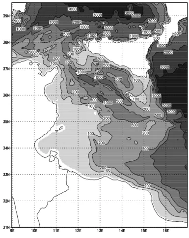
rier for intermediate and deep waters due to an extension of the shelves from Cape Bon in Tunisia and Cape Lilibeo in Italy with two sills closer to the African side (Fig.1). The two Channels are crossed by the waters exchanging from the two Mediterranean basins and organised in a three-layer system. The upper ocean flow is dominated by the eastward bound Modified Atlantic Water (MAW) moving under the influence of the

25

density gradient between the eastern and the western basin, and modified by the in-fluence of the wind forcing and the bottom geometry. The MAW moves eastward from the Strait of Gibraltar along the north African coast forming unstable meanders that often create cyclonic and anticyclonic eddies with spatial scales of ∼200 km (Puillat

(5)

OSD

Full Screen / Esc

et al.,2002). From the Sardinia Channel, two branches of MAW cross the Sicily Strait eastward. The first branch moves along the southern Sicily coast as an energetic and meandering flow called the Atlantic Ionian Stream (AIS, e.g. Robinson et al., 1999; Warn-Varnas et al., 1999; Lermusiaux and Robinson, 2001). Particularly evident in the summer, the eastward flow of AIS in the Sicily Channel is a complicated

mean-5

dering path around three surface thermal features: the Adventure Bank Vortex, the Maltese Channel Crest and the Ionian Shelf Break Vortex. The contact between the fresh MAW of the AIS and the warmer Ionian Sea produces a thermal filament known as the Maltese Front. All these features are partially controlled by topographic effects, internal dynamics and atmospheric forcing (summer winds), although in the Strait, the

10

main variability is baroclinic (Lermusiaux and Robinson,2001). The second branch moves along the Tunisian coast as the African MAW current (Sorgente et al.,2003) characterised by a high seasonal variability and a maximum volume transport in au-tumn (Manzella et al.,1988). In summer, when the AIS reaches its maximum, MAW spreads laterally due to the reduced impact of the wind stress on the MAW/LIW

mix-15

ing (Manzella,1994) and a decrease in salinity minimum because of a lower degree of mixing of the MAW with the surrounding waters. At its maximum, AIS bifurcates southward at the trench past the Island of Pantelleria in a weaker flow that joins with the African MAW current (Lermusiaux and Robinson,2001).

Therefore the circulation of this area is characterised, particularly at the surface, by

20

strong mesoscale signals in the form of eddies, meanders and small-scale gyres whose path and lifetime are mainly influenced by the bathymetric contours, the temperature and salinity gradients and by the meteorological and climatic conditions.

In 2003, the anomalous persistence of the high atmospheric pressure during the summer period, with almost no winds and very high air temperatures (Black et al.,

25

2004) over the western continental Europe and the western basin, determined a strong heatwave event (e.g.,Black et al.,2004;Sch ¨ar et al.,2004). Sutton et al.(2004) re-late this heatwave, as well as other atmospheric extreme events over Western Europe and eastern North America to a multidecadal climatic oscillation of Atlantic sea

(6)

OSD

Full Screen / Esc

face temperatures, known as Atlantic Multidecadal Oscillation (AMO). The summer of 2003 permitted us to evaluate the response of surface waters at a regional scale to anomalous weather conditions driven by large-scale phenomena.

To proceed with the evaluation, a nested high resolution eddy resolving ocean cir-culation model was implemented and a 5-year long run was conducted in the central

5

Mediterranean area. The ocean responses to realistic atmospheric forcing from Jan-uary 2000 to December 2004, have been analysed. The analysis of the time series and variabilty of the dynamic features, with special regards to the SST, which can be easily compared with satellite and in situ data, provides a better understanding of the main time scales of variability and indications about the sensitivity of the surface layer

10

to climate change and atmospheric forcing in this important geographic area. The nu-merical experiment has been conducted within the framework of the European Com-munity project Mediterranean Forecasting System Toward Environmental Prediction (MFSTEP).

After a brief description of the model settings and data analysis, the results are

15

presented in the logical sequence: the analysis of the atmospheric variables involved in the observed phenomena; the analysis of surface heat fluxes and SST as simulated from the ocean model; a comparison of the modelled SST with the remote-sensed one; an overlook on the surface and sub-surface dynamics. In the last section we discuss the results.

20

2 Methods

This section describes the model setup (Sect. 2.1) and explains the analyses per-formed on the model output as well as on the atmospheric parameters (Sect.2.2).

(7)

OSD

Full Screen / Esc

2.1 Model Design

The eddy resolving ocean model, named the Sicily Channel Regional Model (SCRM), has been implemented in the Sicily Channel and surrounding areas with a uniform hori-zontal orthogonal grid resolution of 1/32◦(∼ 3.5 km) in longitude and latitude (257×273 mesh points), while for the vertical, 24 sigma levels (−1≤σ≤0) were used. The sigma

5

levels are bottom following with logarithmic distribution near the surface and bottom. Between the surface and the bottom, levels are equally spaced with a layer thickness of 0.0556, while the topmost layer is 0.0035 thick. The geographical boundaries of the domain are from 9◦E to 17◦E in longitude and from 31◦N to 39.5◦N in latitude. In the present SCRM model domain, the external time step is 4 s, while the internal mode

10

time step is 120 s.

The basic numerical formulation of the nested ocean circulation model is based upon the POM (Princeton Ocean Model), a three-dimensional primitive equation model (Blumberg and Mellor, 1987). POM solves the equations of continuity, momentum, conservation of temperature, salinity and assumes hydrostaticity and the Boussinesq

15

approximation (Blumberg and Mellor,1987). The equation of state is an adaptation of the UNESCO equation of state revised by Mellor (1991). The vertical mixing coe ffi-cients are calculated using theMellor and Yamada(1982) turbulence closure scheme, while the horizontal diffusion terms are calculated using theSmagorinsky (1993) for-mula. Time integration is done with a split explicit scheme in which the barotropic and

20

baroclinic modes are integrated separately.

The requirement of high resolution SCRM is that it should be capable of resolving the mesoscale features, such as fronts and other hydrological phenomena characterized by periods from 3 to 10 days (Manzella et al.,1988), while their horizontal dimension is of the order of the local internal Rossby deformation radius, ∼19 km. The chosen

25

model grid size is sufficiently shorter to resolve the main features and steep bathymetry areas that can not be simulated by a coarse resolution model. SCRM is driven at the lateral open boundaries by the large, basin scale model using the nesting technique.

(8)

OSD

Full Screen / Esc

It improves the ability to simulate coastal shelf processes producing a more detailed description of the circulation. The basin scale model, called Ocean General Circulation Model (OGCM), is based on a modified version of the Modular Ocean Model-MOM (Pacanowski et al., 1990) implemented in the Mediterranean basin with a horizontal resolution of 1/8◦degrees and 31 levels in vertical (Pinardi and Masetti,2000;Demirov

5

and Pinardi,2002).

The model bathymetry is based on the U.S. Navy 1/60◦ Digital Bathymetric Data Base (DBDB1) by bilinear interpolation onto the SCRM grid. Additional light smooth-ing was applied to reduce the sigma coordinate pressure gradient error (Mellor et al., 1994). The resulting model bathymetry, as well as the model domain, is shown in

10

Fig.1. The maximum depth is ∼3500 m, while the minimum was set to be 5 m.

The model was spun up from a stationary state obtained by forcing the SCRM in a yearly perpetual mode for 8 years, based on the year 2000. The boundary conditions were provided at the surface by six-hour sea surface fluxes (wind stress, heat and fresh water) from ECMWF analyses fields, and at the lateral boundaries by the OGCM daily

15

mean analyses.

2.1.1 Surface boundary conditions

An important characteristic of SCRM is the implementation of a one-way interactive air-sea scheme with high frequency atmospheric forcing. It consists of using a well-tuned set of bulk formulæ(Castellari et al., 1998) for the computation of momentum, heat

20

and freshwater fluxes at the air-sea interface. These fluxes depend on the six-hourly (00:00; 06:00; 12:00; 18:00 UTC) 0.5◦ECMWF operational analysis of the atmospheric parameters (wind at 10 m above sea level., air temperature at 2 m a.s.l., cloud cover, specific humidity and pressure). The SST, needed for the surface flux computation, was obtained using the value predicted by the ocean model itself. The momentum, heat

25

and freshwater fluxes were then mapped on the regional model grid through bilinear interpolation and linearly interpolated in time for each model time step.

(9)

OSD

Full Screen / Esc

The surface boundary condition for the momentum fluxes (wind stress) used is:

K_M ∂U ∂z z=η = τ ρ₀, (1)

where K_Mis the vertical kinematic viscosity coefficient for water and τ is the wind stress calculated from the surface winds using the following equation:

τ= (τ_x, τ_y)= ρ_AC_D|W |(Wx, Wy). (2)

5

Here W_x and W_y are the wind components; ρ_A is the density of moist air as a func-tion of air pressure, temperature and relative humidity; ρ₀ is the reference density for the sea water (1025 kg m−3), |W | is the module of wind velocity at 10 m a.s.l.,

C_D=C_D(T_A, T_S, W ) is the drag coefficient calculated as function of the wind amplitude

(W ), the air (T_A) and sea surface temperatures (SST ) through the polynomial

approx-10

imation given by Hellerman and Rosenstein (1983). SST is taken directly from the ocean model, while T_Ais taken from the atmospheric input data.

The surface boundary condition for potential temperature takes the following form:

K_H ∂Θ ∂z _z_=η = Q_tot ρ₀c_p+ ∂Q ∂T 1 ρ₀c_p(Tz=0− Tz=η), (3)

where K_H is the vertical heat diffusivity for water, c_p (4186 JKg−1K−1) is the specific

15

heat capacity of pure water at constant pressure and Q_tot is the net heat flux or total heat budget. The second term on the right-hand side of Eq. (3) is the correction ( Za-vatarelli et al.,2002) used to force the heat flux in order to produce a SST consistent with the monthly climatology MED6 (Brasseur et al.,1996), where T_z₌₀is the monthly averaged climatological sea surface temperature obtained from the MED6 data

inter-20

polated into the model grid, T_z_=η is the predicted SST by the SCRM itself at the first level. Sensitivity studies performed on the ocean model indicate an optimal value for

∂Q/∂T to be 30 Wm−2C−1.

(10)

OSD

Full Screen / Esc

The total heat budget at the air-sea interface is given by the following equation:

Q_tot= Q_s− Q_b− Q_e− Q_h, (4)

where Q_s is the solar radiation flux, computed according to theReed(1977) parame-terization, Q_bis the net long-wave radiation flux, according toBignami et al.(1995), Q_e is the latent heat flux, mainly due to the evaporative processes, and Q_h is the sensible

5

heat flux, which is driven by the difference between the air and sea surface temper-atures. In particular, the sensible and latent heat fluxes were computed according to classical formulas, with the turbulent exchange coefficients computed followingKondo (1975). In the discussion of the upward fluxes, Q_b, Q_e and Q_hare positive for energy gained by the atmosphere.

10

For the salinity flux surface boundary condition we consider the following equation in agreement withZavatarelli et al.(2002):

K_H ∂S ∂z _z_=η=(E −P )Sz=η+∆σ(1) H α(Sz=0−Sz=η), (5)

where S_z_=η is the model predicted surface salinity field, E=Q_e/L_e is the evaporation rate calculated interactively, L_e is the latent heat of evaporation. The monthly

precip-15

itation rate (P ) are obtained from Legates and Willmott (1990) global dataset, while

S_z₌₀ is the monthly mean climatological surface salinity from MED6. In the SCRM do-main, the runoff has not been included because any river can be considered a relevant source of fresh water. The second term on the right-hand side of Eq. (5) is the salt correction used to ensure the fresh water flux produces a sea surface salinity field

con-20

sistent with the climatology. Here∆σ(1)H the thickness of the surface layer and α is the relaxation time. The term∆σ(1)(H/α) has been chosen to be equal to 0.7 m day−1. All of the above forcings were bilinearly interpolated in space onto the model grid and linearly in time to the model time step.

(11)

OSD

Full Screen / Esc

2.1.2 Lateral open boundary conditions

At the lateral open boundaries, the model receives information of temperature, salinity and total velocity fields by one-way, off-line nesting to the OGCM that covers the whole Mediterranean Sea. The grid-nesting ratio between the two models is 2.0. A detailed description of the nesting procedure can be found inSorgente et al.(2003).

5

The following explanation of the boundary conditions assumes that U and V are nor-mal and tangential components of velocity to the boundary, respectively, i.e. it applies directly for the western and eastern boundaries. At the SCRM lateral open boundaries, the vertically integrated normal velocity is specified at each time step through the fol-lowing equation, initially proposed byFlather(1976) and modified byMarchesiello et al.

10

(2001) andPinardi et al.(2003):

¯

U= ¯U_OGCMint (H+η

int OGCM) (H+η) +ε s g H+η(η −η int OGCM), (6) where ¯ U_OGCMint = 1 H+ηint_OGCM η Z −H U_OGCMint d z

and the subscript OGCM stands for the coarse model data interpolated (superscript

15

int) onto the SCRM grid. The term ε is equal to+1 for eastern and northern, −1 for western and southern open boundaries. The term ¯U is the vertically integrated velocity

on the open boundary, H is the fine resolution bottom depth, ηint_OGCM is the coarse free surface elevation interpolated on the fine model resolution and g (Eq.6) is the gravitational acceleration. The tangential barotropic velocities at the boundaries are

20

simply equalized: ¯

V = ¯V_OGCMint

(12)

OSD

Full Screen / Esc

The internal mode velocities U and V (normal and tangetial), at the open boundaries of SCRM, are fully specified by a bilinear interpolation of the daily mean coarse resolution model fields into the high resolution model grid:

U = U_OGCMint , V = V_OGCMint .

5

To update the temperature and salinity fields an upstream advection scheme is used when the velocity is directed outward of the modelling area:

∂Θ ∂t + U ∂Θ ∂n = 0, ∂S ∂t + U ∂S ∂n = 0,

where n is the normal at the boundary.

10

In cases of inflow through the open boundaries, the three-dimensional temperature and salinity fields are prescribed from the values of the coarse model solution, interpo-lated on the nested open boundaries:

Θ = Θint OGCM,

S= S_OGCMint .

15

The free surface elevation is not nested (zero gradient boundary condition):

∂η ∂n = 0

2.2 Wavelet analysis

Two dimensional fields of variables either from ECMWF atmospheric input or from the SCRM output were averaged to obtain time series of daily spatial averages. In addition,

20

(13)

OSD

Full Screen / Esc

we calculated monthly average values for the whole 5-year period for each variable. In order to separate the seasonal (i.e. the intra-annual variability mainly related to the orbital cycle) from the non-seasonal variability (interannual and high frequency vari-ability), we subtracted the 5-year average monthly value from the daily time series and normalized the results by monthly standard deviation:

5

x_a= x− xm

σ_m , (7)

where x is the daily datum, x_m is the climatological (2000–2004) monthly mean for a corresponding month and σ_m is the related monthly standard deviation.

In order to analyse the variability of the calculated time series, we performed both the Fourier Transform (FT) and the Continuous Wavelet Transform (CWT). The CWT is a

10

useful instrument to analyse time series data with a strong non-stationary component. The CWT allows exceptional localization, both in the time domain with translations of the mother wavelet (defined below) and in the frequency domain with its dilations, while the FT is only able to recognise the location and the magnitude of maxima and minima in the frequency domain. However the FT remains very appropriate for the analysis

15

of stationary data, which does not require time localization information or to get an overview of the main components of a signal, as in our analysis.

Before performing the CWT and the FT we have removed the trend from the anoma-lies data to reduce the presence of spurious low frequency signals. By definition, a mother wavelet is a function with a zero mean and must be defined in both time and

20

frequency dimensions. To calculate the CWT we have chosen the Morlet wavelet as the mother wavelet, which is very useful for oceanographic data both in its real or com-plex forms (Torrence and Compo,1998;Massel,2001;Cromwell,2001). The complex Morlet wavelet function is defined as follows:

ψ₀(η)= π−1/4ei ωoη_e−η

2

/2_, ₍₈₎

25

where η is the nondimensional “time” parameter from which depends the function and

ω_o is the non dimensional frequency.

(14)

OSD

Full Screen / Esc

As inTorrence and Compo(1998) we define the Continous Wavelet Transform as the convolution of our discrete time series x_n, in our case constituted by the x_a elements, with dilations and translations of the mother wavelet function ψ₀.

In the wavelet plots, in which wavelet power was drawn in the two dimensional time-frequency domain, we also drew the 95% significance level contours (thick black lines)

5

and the area known as Cone Of Influence (COI), that delimits the area in which there is no edge effect (thin black line delimiting a triangular-shaped area). The edge effect is an error present in the spectral analyses and related to the proximity of boundaries in the time dimension. The significance levels have been estimated comparing the wavelet spectrum to a red-noise signal (commonly used for geophysical time series),

10

computed on the basis of the lag-1 autocorrelation of the same time series.

3 Results

The results of the wavelet analyses performed on atmospheric variables (Sects. 3.1, 3.2), on surface heat fluxes (Sect. 3.3) and on SST (Sect. 3.3) are dis-cussed in this section, as the most noticeable monthly values for each parameter, and

15

when necessary, the seasonal trends. The parallel observation of the time-frequency (wavelet and FFT plots) data and of the raw time series, gives a complete picture of the variability of the analysed variables. In Sect.3.5we report the maps and some obser-vation about water stratification and surface currents modifications during the summer 2003.

20

3.1 Air temperature

In the summer of 2003 the air temperature at 2 m reached values above 35 degrees Celsius in June, July and August (JJA) in many European areas. This high tempera-ture was mainly caused by the prevalence of anticyclonic conditions (Black et al.,2004). Furthermore, the JJA monthly means of air temperature over central Europe reached

25

(15)

OSD

Full Screen / Esc

values up to ∼5◦C warmer than in the last 150 years climatology. Over a larger Euro-pean area, values have been recorded as ∼3◦C warmer in the 1961–1990 climatology (Sch ¨ar et al.,2004).

From our analyses, in respect to the 2000-2004 climatology, in the 2003 JJA months, the daily anomalies time series of air temperature over the SCRM domain reached the

5

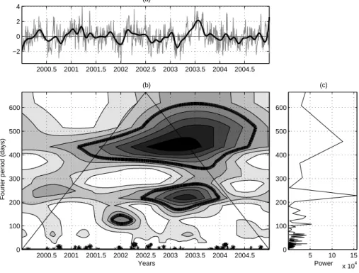
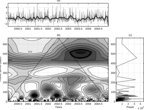
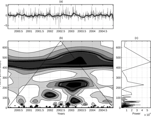
highest values of the entire period (up to+3−4◦C). In Fig.2the normalized anomalies time series, the wavelet spectrum and the periodogram (Fourier spectrum) relative to this parameter are shown, respectively. The presence of two distinct anomalies at two distinct frequencies (Fourier period of ∼450 and ∼220 days) are observed, temporally superimposed and centred in the year 2003. We observe that both the signals reach

10

their maximum magnitude in a time period situated between the warm anomalies of summer 2003 and January/February (JF) 2003, when the coldest anomaly of the whole period is recorded. We may also notice a reduction of the high frequency signal in summer 2003, mainly due to the persistence of anticyclonic conditions, whose effect is in fact reducing the short term variability. Another weak but statistically significant

15

signal, at a shorter Fourier period (120 days), is consistent with anomalous negative values of air temperature in December 2001/January 2002.

3.2 Wind stress

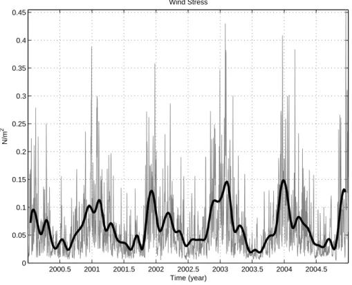
The wind stress time series, computed from the ECMWF atmospheric fields and used as input in the simulation, is shown in Fig. 3. The highest wind stress monthly

20

values are reached in February and December 2003 (respectively 0.16×10−2 and 0.15×10−2 Nm−2), while the lowest are reached in the summer months of the same year. This last datum is consistent with the computed high values of air and sea sur-face temperature (see below) for this period.

The spectral analyses performed on the anomalies series for the wind stress intensity

25

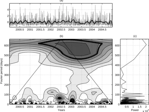
(Fig.4) show that a great part of non-seasonal variability is concentrated at the highest frequencies, with the great exception of the very long wave signal temporally coincident

(16)

OSD

Full Screen / Esc

with the air temperature anomalies of 2003, although it was partially outside of the COI. 3.3 Surface heat fluxes

The daily and monthly averaged time series of solar radiation, upward (i.e. the sum of

Q_e, Q_band Q_hcomponents) and net heat fluxes, are shown in Fig.5.

The solar radiation time series (Fig.5a) shows a strong seasonal variability

charac-5

terised by a minimum value in December for all years, with the exception of January 2003 and January 2004. The annual averages ranged from 208 Wm−2 to 210 Wm−2 with a very low interannual variability. In performing the wavelet analysis, no significant anomaly was found with the exception of a weak signal at the beginning of 2003 (not shown).

10

The upward heat flux (Fig.5b) appeared to have a more complicated structure com-pared to the solar radiation. This was mainly due to the strong dependence of upward heat flux on atmospheric variables such as air temperature and wind intensity, as seen previously. The upward fluxes ranged from 227 Wm−2from the year 2001 to 239 Wm−2 from 2004. In respect to the 5-year climatology, we calculated the strongest positive

15

monthly anomalies in February 2003 (+1.54, adimensional). They were calculated by subtracting the monthly mean from the monthly climatological value and then normal-ising by standard deviation, in a similar way as for the daily anomalies time series. The strongest negative (−1.62 and −1.63) monthly anomalies were in March 2001 and June 2003. A strong decrease of fluxes in comparison to the 5-year climatology was

20

also noticeable from the months of April to November 2003, with the absolute minima in JJA.

A strong interannual variability on a monthly basis, as well as a moderate variability on annual basis is therefore intuitive, but no conclusion can be drawn on the frequen-cies and periods of these deviations when considering the averaged values only. The

25

analysis of the spectra of the anomalies time series (wavelet and fourier spectra) pro-vide this important information.

In Fig.6the daily anomalies time series (normalized by standard deviation) of upward 99

(17)

OSD

Full Screen / Esc

fluxes and the spectral analyses of data are shown.

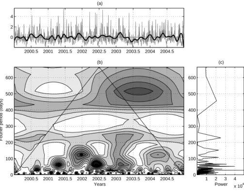
The two spectra of Fig. 6b and c indicate the presence of a significant long wave signal in the anomalies time series with a Fourier period of ∼450/500 days. This signal coincided with a strong increase of upward fluxes in the winter-spring 2003 and their decrease in summer 2003. In the rest of the year it was also observed in the

5

averaged values. This long wave signal had a very good agreement with other sea surface and atmospheric anomalies we registered in the same time-frequency location (see below), although it is located just out of the COI. The rest of variability of the anomalies time series were located at the highest frequencies and is related mainly to the high frequency atmospheric variability.

10

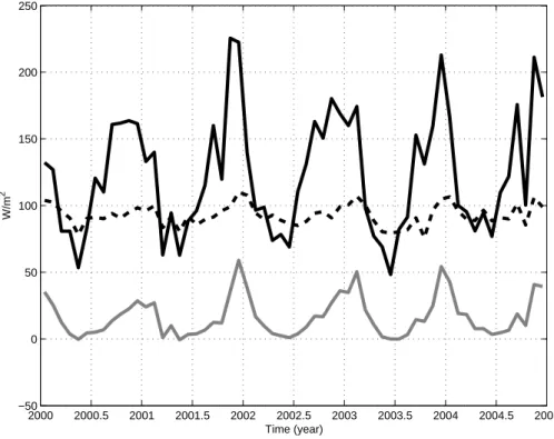
In Fig.7 the monthly time series of the three components of upward flux was com-pared. It is clear that the main component is the Latent Heat flux (Q_e), followed by the Longwave Radiation (Q_b), while the Sensible Heat (Q_h) is the less important in terms of total budget.

The latent heat flux reached its maximum seasonal values in the autumn and

win-15

ter months (remember that for the Q_e, Q_b and Q_h terms, positive values indicated a flux from the sea surface to the atmosphere). The absolute maximum was reached in November and December 2001 with 222 and 225 Wm−2 respectively, while the mini-mum was reached in June 2003 with 48 Wm−2. This last minimum corresponds to the major anomaly observed for the total upward heat fluxes. Also the Q_b and Q_h fluxes

20

had their seasonal maxima in the autumn and winter months. Very low, 3-month av-eraged values had been reached, for both terms, in JJA 2003 with ∼80 Wm−2 and ∼1 Wm−2, respectively.

The spectral analyses of the anomalies series suggests (Figs.8,9and10), all three components to be involved, to a various extent, in the surface anomalies of 2003. While

25

in absolute terms the Q_e component underwent the main decrease in summer 2003, and therefore it was the principally responsible for that anomaly, in terms of wavelet power, which can be considered in this case a measure of intrinsic variability, the Q_b and above all the Q_h component showed the strongest anomalies.

(18)

OSD

Full Screen / Esc

The net heat flux values (Fig.5c), 5-year averaged, resulted positively (i.e. the sea gain heat) in the months from April to August, with a maximum value of 166 Wm−2 in June. Values became negative in the other months with a minimum of −251 Wm−2 in December. The behaviour of the net heat flux, calculated as described in Eq. (4), as well as its non seasonal variability, is logically driven by the upward heat flux,

con-5

sidering the very low interannual variability of the solar radiation term. The wavelet spectrum for the net heat flux anomalies was similar to the upward flux (not shown). 3.4 Sea surface temperature

Strictly related to the previously seen surface heat fluxes and atmospheric parameters, the SST monthly time series (Fig.13a) simulated by the model shows a strong annual

10

cycle and a somewhat weaker interannual signal, mainly related to the strong heat gain from the summer 2003.

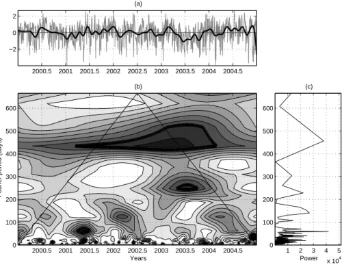
The spectral analysis of the daily anomalies time series (Fig. 11) shows a main anomaly with a Fourier period of ∼450 days, which is consistent with the heatwave affecting Europe and the Mediterranean area during the summer 2003. Although it cuts

15

off the boundary of the COI, this wave has a very high level of significance (greater than 95%). Another weak signal, related to a negative anomaly, is detected at the beginning of the time series, but it was not considered since it is entirely out of the COI of the wavelet spectrum and has a low significance level.

It is interesting to observe that the main wavelet signal was not limited to summer

20

2003, but with a 95% of significance level (thick black line) it extended from the middle of 2002 to the beginning of 2004, covering more than a 1.5 year interval. Furthermore, by considering only the highest magnitude of the spectrum, the main wavelet signal was reached between December 2002 and August 2003, including also the strong heat loss in winter 2003 (see also the wind stress and the upward heat fluxes spectra) and

25

the heat wave of summer 2003. The presence of statistically significant signals at high frequencies during the entire series, although they register very low power spectra, was mainly due to the very high autocorrelation (lag-1 autocorrelation >0.95) of the

(19)

OSD

Full Screen / Esc

SST time series.

Figure12illustrates the maps of the SST monthly anomalies (August), from 2001 to 2004, as simulated from the model. The anomalies maps are computed in comparison to the 5-years climatology. It is clear that, in 2003, the main overheating occurred in the northwestern area of the SCRM domain.

5

In order to compare the simulated SST (temperatures are interpolated from sigma levels to the 0.5 m zeta level) to real observed values, the means computed from satellite SST monthly maps have been compared with the SST time series simulated from the SCRM.

The AVHRR Oceans Pathfinder SST data are derived from the 5-channel Advanced

10

Very High Resolution Radiometers (AVHRR) on board of the NOAA –7, –9, –11, –14, –16 and –17 polar orbiting satellites. The monthly averaged data for the ascending pass (daytime) on equal-angle grids of 8192 pixels/360 degrees (nominally referred to as the 4 km resolution) have been used.

In Fig. 14 the AVHRR SST values for the month of August, covering the entire

15

Mediterranean area are shown. The strong increase of SST values in 2003 is clearly visible. We can also see that the main region of overheating is located in the north-western area, as simulated from the ocean model in the SCRM domain.

In Fig. 13a we may observe that the computed SST is in a good agreement with the satellite monthly data, with an average offset between the two series of ∼+0.4◦C.

20

The difference between the two time series, shown in Fig.13b, ranges from −0.5◦C to 1.3◦C, reaching the highest and lowest values in agreement with the surface anomalies of 2003. The satellite monthly means are generally colder than the model output, with the exception of the summer 2003 when the model underestimated the real SST temperature, assuming no error for the remote-sensed data.

25

The behaviour of the simulated SST, in comparison to the real SST values, could be due to the relaxation term in the heat flux calculations (Eq. 3), that generates a smoothing effect on the upward fluxes signal, underestimating the extreme anomalies, both positive and negative.

(20)

OSD

Full Screen / Esc

3.5 Surface layer: AIS and coastal upwelling

The combined effects of above average air temperatures and low wind intensities in the summer 2003 determined a strong water stratification and a very reduced coastal up-welling, as is seen in Fig.15, in which the JJA averaged temperatures are plotted from 2001 to 2004 (the omitted 2000 year subplot is analogue to the 2001 subplot), along

5

a cross-section at 13◦E of longitude, from the middle Sicily Channel to the southern Sicily coast. The trend of isoterms in the 2003 subplot in proximity of the Sicily coast is particularly noticeable. If compared with the other subplots they do not show the characteristic inclination toward the surface at all that would indicate the presence of coastal upwelling. It is also interesting to observe that the temperature deviations were

10

confined to the upper layer, from the surface to ∼25 m of depth.

In Fig. 16 we show the JJA averaged maps of subsurface (30 m depth) currents intensity and direction, on the AIS area of interest. The usual path and meandering behaviour of the AIS, as described by different authors (e.g. Robinson et al., 1999; Warn-Varnas et al., 1999; Lermusiaux and Robinson, 2001), is visible in the three

15

subplots referred to the 2001, 2002 and 2004 years (Fig.16a, b, d; the year 2000 not shown is substantially consistent with 2001, 2002 and 2004 subplots). The AIS flow was strongly modified in the summer 2003, as is clearly visible from the related subplot (Fig.16c). The AIS branch flowing under the southern Sicily coast is reduced both in magnitude as well as in its characteristic meandering flow. On the contrary, the flow

20

of the African MAW current (Sorgente et al., 2003), flowing along the Tunisian shelf, seems to be intensified in respect to other four years.

4 Conclusions

In summer 2003 the air temperature reached its highest values in the last 150 years in many European continental areas. Air temperature also reached very high values over

25

the SCRM domain in comparison to the 5-year climatology. The performed wavelet 103

(21)

OSD

Full Screen / Esc

analysis shows that there are two main signals temporally superimposed at two di ffer-ent frequencies that are probably both involved in the 2003 heat wave anomalies.

Considering the daily anomalies series of the wind stress, its variability seems to be dominated by a high frequency signal. Conversely, the spectral analyses show a very low frequency peak centered in the year 2003, consistent with the observed

5

phenomena, although it is partially outside of the COI of the wavelet plot. This long wave signal coincides with high values of wind stress in winters 2003 and 2004 and low values in summer 2003 that are probably related to the same SST anomaly described above.

The interannual variability of surface heat fluxes seems to be driven by the values

10

of upward fluxes because of the strong seasonality and periodicity of the downward heat transport (solar radiation). All three components of upward fluxes were involved in the anomalies of 2003, i.e. all the evaporation processes, the longwave radiation and the sensible heat flux. Although Q_h is the least important component in absolute terms, while Q_eis the main contributor (i.e. the component with the maximum absolute

15

decrease for that period), the former is affected by the main decrease in percentage terms. The low frequency signal of the total upward fluxes is mainly related to the air temperature parameter and partially to the wind stress, while the high frequency part is in relationship with the wind stress variability.

The analyses of other atmospheric parameters (e.g. the cloud cover and the

rela-20

tive humidity) indirectly involved in the described surface anomalies did not show any particular signal. It is interesting to note that the absence of significant anomalies for the relative humidity parameter in the summer of 2003 means an increase of abso-lute humidity, because of the elevated air temperature. The difference between the value of the saturated absolute humidity at the sea surface and the air humidity, driving

25

the latent heat flux, was reduced, which could possibly explain the strong decrease of observerd Q_e.

Our analyses show that the computed SST, calculated in the 5-year interannual ex-periment on the Central Mediterranean Sea, fits well the AVHRR data with a positive

(22)

OSD

Full Screen / Esc

bias of+0.4◦C (i.e. the model is a little warmer than the satellite). The difference turns

out to be greater in correspondence with extreme values, either positive or negative. This could be due to the presence of the relaxation term in the computation of upward fluxes, but the term is necessary for a realistic SST estimation (Zavatarelli et al.,2002). However, as observed in the SST wavelet spectrum, the effects of the 2003 European

5

heat wave on the sea surface are well described and are defined in the time-frequency domain. The long-wave SST interannual signal related to this event is not timewise lim-ited to the summer 2003, but it extends back to the winter of the same year when the SST values of almost 2◦C lower than the 5-year climatological average were recorded. The SST anomalies simulated with the SCRM seem to be related in the Sicily Strait

10

area mainly to the air temperature and less to the wind stress intensity. The atmo-spheric anomalies that Sutton et al. (2004) relates to very large-scale atmospheric forcings like the AMO, are correlated at regional scale with the surface heat upward fluxes, which show their consistency with the low frequency signal. Furthermore, the spectral analyses show that the longwave signal is not timewise limited to the summer

15

months of 2003, but it is part of a longer lasting anomaly from autumn 2002 to winter 2003, in agreement with negative anomalies of SST values and positive anomalies of upward fluxes. The Fourier period of this signal suggests that the anomaly must have covered a larger time window than only the few summer months of 2003.

The same atmospheric forcing determining the heat fluxes and SST anomalies is

20

probably related to the AIS and African MAW fluxes modifications observed in the same period, as well as on the reduced upwelling and on the more intense water stratification along the southern Sicily coast. Keep in mind the importance of AIS flux and coastal upwelling, for instance in the reproduction strategies of some commercially important small-pelagic species (Garcia-Lafuente et al.,2005).

25

Further analyses, also including ecological and biological data, will enable us to determine the ecological impact of the observed modifications of SST and verti-cal/horizontal dynamics.

Acknowledgements. Wavelet software was provided by C. Torrence and G. Compo, and is

(23)

OSD

Full Screen / Esc

available at URLhttp://paos.colorado.edu/research/wavelets/.

The AVHRR Oceans Pathfinder SST data have been provided by the Physical Oceanogra-phy Distributed Active Archive Center (PO.DAAC) at the NASA Jet Propulsion Laboratory, Pasadena, CA.http://podaac.jpl.nasa.gov.

This work has been realised in the framework of EU MFSTEP project (EVK3-2001-00174) and

5

the EU Marie Curie Development Host Fellowship, ODASS project (HPMD-CT-2001-00075).

References

Agostini, V. N. and Bakun, A.: “Ocean Triads” in the Mediterranean Sea: Physical mechanisms potentially structuring reproductive habitat suitability (example application to European an-chovy, Engraulis encrasicolus), Fish. Oceanogr., 11, 129–142, 2002. 87

10

Astraldi, M., Conversano, F., Civitarese, G., Gasparini, G. P., Ribera dAlcal, M., and Vetrano, A.: Water mass properties and chemical signatures in the central Mediterranean region, J. Marine Syst., 33–34, 155–177, 2002.

Bakun, A.: Patterns in the ocean: ocean processes and marine population dynamics, California Sea Grant, La Jolla, California, 323 pp., 1996. 87

15

Beniston, M. and Diaz, H. F.: The 2003 heat wave as an example of summers in a greenhouse climate? Observations and climate model simulations for Basel, Switzerland, Global and Planetary Change, 44, 73–81, 2004.

Bignami, F., Marullo, S., Santoleri, R., and Schiano, M. E.: Longwave radiation budget in the Mediterranean Sea, J. Geophys. Res., 100, 2501–2514, 1995. 93

20

Black, E., Blackburn, M., Harrison, G., Hoskins, B., and Methven, J.: Factors contributing to the summer 2003 European Heatwave, Weather, 59(8), 217–222, 2004. 88,97

Blumberg, A. F. and Mellor, G.: A description of a three-dimensional coastal ocean circulation model, in: Three-dimensional Coastal Ocean Models, Coastal Estuarine Science, edited by: Heaps, N. S., Americ. Geophys. Union, pp. 1–16, 1987. 90

25

Brasseur, P., Beckers, J. M., Brankart, J. M., and Schoenauen, R.: Seasonal temperature and salinity fields in the Mediterranean Sea: Climatological analyses of an historical data set, Deep-Sea Res. I, 43(2), 159–192, 1996. 92

Brett, J. R.: Temperature – Fishes, in: Marine ecology. Volume I. Environmentals factors. Part I, edited by: Kinne, O., pp. 514–616, Wiley Interscience, Glasgow, 1970. 86

30

(24)

OSD

Full Screen / Esc

Castellari, S., Pinardi, N., and Leaman, K.: A model study of air-sea interaction in the Mediter-ranean Sea, J. Marine Syst., 18, 89–114, 1998. 91

Cromwell, D.: Sea surface height observations of the 34◦N “waveguide” in the North Atlantic, Geophys. Res. Lett., 19(28), 3705–3708, 2001. 96

Demirov, E. and Pinardi, N.: Simulation of the Mediterranean Sea circulation from 1979 to

5

1993: Part I. The interannual variability, J. Marine Syst., 33–34, 23–50, 2002. 91

Flather, R. A.: A tidal model of the northwest European continental shelf, Mem. Soc. R. Sci. Liege, 6(X), 141–164, 1976. 94

Garcia-Lafuente, J., Vargas, J. M., Criado, F., Garcia, A., Delgado, J., and Mazzola, S.: Assess-ing the variability of hydrographic processes influencAssess-ing the life cycle of the Sicilian Channel

10

anchovy, Engraulis encrasicolus, by satellite imagery, Fisheries Oceanography, 14(1), 32– 46, 2005. 87,105

Gasparini, G. P., Ortona, A., Budillon, G., Astraldi, M., and Sansone, E.: The effect of the Eastern Mediterranean Transient on the hydrographic characteristics in the Strait of Sicily and in the Tyrrhenian Sea, Deep-Sea Res. I, 52, 915–935, 2005.

15

Hellerman, S. and Rosenstein, M.: Normal monthly windstress over the world ocean with error estimates, J. Phys. Oceanogr., 13, 1093–1104, 1983. 92

Kondo, J.: Air-sea bulk transfer coefficients in diabatic conditions, Bound. Layer Meteor., 9, 91–112, 1975. 93

Legates, D. R. and Wilmott, C. J.: Mean seasonal and spatial variability in gauge correctd global

20

precipitation, Int. J. Climatol., 10, 111–127, 1990. 93

Lermusiaux, P. F. J. and Robinson, A. R.: Features of dominant mesoscale variability, circulation patterns and dynamics in the Strait of Sicily, Deep-Sea Res. I, 48, 1953–1997, 2001. 88,

103

Levi, D., Andreoli, M. G., Bonanno, A., Fiorentino, F., Garofalo, G., Mazzola, S., Norrito, G.,

25

Patti, B., Pernice, G., Ragonese, S., Giusto, G. B., and Rizzo, P.: Embedding sea surface temperature anomalies into the stock recruitment relationship of red mullet (Mullus Barbatus L. 1758) in the Strait of Sicily, Sci. Mar., 67 (Suppl. 1), 259–268, 2003. 87

Manzella, G. M. R.: The seasonal variability of the water masses and transport through the Strait of Sicily. Seasonal and interannual variability of the Western Mediterranean Sea, La

30

Violette ed. AGU, 33–45, 1994. 88

Manzella, G. M. R., Gasparini, G. P., and Astraldi, M.: Water exchange between the eastern and western Mediterranean through the Strait of Sicily, Deep-Sea Res. I, 35, 1021–1035,

(25)

OSD

Full Screen / Esc

1988. 88,90

Marchesiello, P., McWilliams, J. C., and Shchepetkin, A.: Open boundary conditions for longterm integration of regional oceanic models, Ocean Modelling, 3, 1–20, 2001. 94

Massel, S. R.: Wavelet analysis for processing of ocean surface wave records, Ocean Engi-neering, 28, 957–987, 2001. 96

5

Mellor, G. L.: An equation of state for numerical models of oceans and estuaries, J. Atmos. Oceanic Tech., 8, 609–611, 1991. 90

Mellor, G. L. and Blumberg, A. F.: Modelling vertical and horizontal diffusivities with the sigma coordinate ocean models, Mon. Wea. Rev., 113, 1379–1383, 1985.

Mellor, G. L., Ezer, T., and Oey, L. Y.: The pressure gradient conundrum of sigma coordinate

10

ocean models, problems, J. Atmos. Oceanic. Tech., 11, 1126–1134, 1994. 91

Mellor, G. L. and Yamada, T.: Developement of a turbulence closure model for geophysical fluid problems, Rev. Geophys. Space Phys., 20, 851–875, 1982. 90

Molcard, A., Gervasio, L., Griffa, A., Gasparini, G. P., Mortier, L., and Tamay, M. ¨O.: Numerical investigation of the Sicily Channel dynamics: density currents and water mass advection, J.

15

Marine Syst., 36, 219–238, 2002.

Pacanowski, R. C., Dixon, K., and Rosati, A.: Readme file for GFDL-MOM 1.0, Geophys. Fluid Dyn. Lab., Princeton, N.J., 1990. 91

Pinardi, N., Allen, I., Demirov, E., De Mey, P., Korres, G., Lascaratos, A., Le traon, P. Y., Maillard, C., Manzella, G. M. R., and Tziavos, C.: The Mediterranean ocean forecasting system: first

20

phase of implementation, Ann. Geophys., 21, 3–20, 2003. 94

Pinardi, N. and Masetti, E.: Variability of the large scale general circulation of the Mediter-ranean Sea from observations and modelling: a review, Palaeogeography, Palaeoclimatol-ogy, PalaeoecolPalaeoclimatol-ogy, 158, 153–173, 2000. 91

Puillat, I., Taupier-Letage, I., and Millot, C.: Algerian eddies lifetime can near 3 years, J. Marine

25

Syst., 31, 245–259, 2002. 87

Reed, R. K.: On estimating insolation over the ocean, J. Phys. Oceanogr., 7, 482–485, 1977.

93

Robinson, A. R., Sellschopp, J., Warn-Varnas, A., Leslie, W. G., Lozano, C. J., Haley Jr., P. J., Anderson, L. A., and Lermusiaux, P. F. J: The Atlantic Ionian Stream, J. Marine Syst., 20,

30

129–156, 1999. 88,103

Ruardij, P., van Haren, H., and Ridderinkhof, H.: The impact of thermal stratification on phy-toplankton and nutrient dynamics in shelf seas: a model study, J. Sea Res., 38, 311–331,

(26)

OSD

Full Screen / Esc

1997. 87

Sch är, C., Vidale, P. L., L üthi, D., Frei, C., H äberli, C., Liniger, M. A., and Appenzeller, C.: The role of increasing temperature variability in European summer heatwaves, Nature, 427, 332–336, 2004. 87,88,98

Smagorinsky, J.: Some historical remarks on the use of nonlinear viscosities, in: Lare eddy

sim-5

ulation of complex engineering and geophysical flows, edited by: Galperin, B. and Orszag, S. A., pp. 3–36, Cambridge Univ. Press, 1993. 90

Sorgente, R., Drago, A. F., and Ribotti, A.: Seasonal variability in the Central Mediterranean Sea circulation, Ann. Geophys., 21, 299–322, 2003. 88,94,103

Sutton, R. T. and Hodson, D. L. R.: Atlantic Ocean Forcing of North American and European

10

Summer Climate, Science, 309, 115–118, 2004. 88,105

Torrence, C. and Compo, G. P.: A practical guide to wavelet analysis, Bull. Am. Meteor. Soc., 79, 61–78, 1998. 96,97

Warn-Varnas, A., Sellschopp, J., Haley Jr., P. J., Leslie, W. G., and Lozano, C. J.: Strait of Sicily water masses, Dynamics of Atmospheres and Oceans, 29, 437–469, 1998. 88,103

15

Zavatarelli, M., Pinardi, N., Kourafalou, V. H., and Maggiore, A.: Diagnostic and prognostic model studies of the Adriatic Sea general circulation: Seasonal variability, J. Geophys. Res., 107(C1), 4-1–4-20, doi:10.1029/2000JC000210, 2002. 92,93,105

(27)

OSD

Full Screen / Esc

Fig. 1. SCRM domain and model bathymetry obtained from U.S. Navy DBDB1 by bilinear

interpolation into the regional model grid. Depth in metres.

(28)

OSD

Full Screen / Esc

Printer-friendly Version Interactive Discussion 2000.5 2001 2001.5 2002 2002.5 2003 2003.5 2004 2004.5 −2 0 2 4 (a)

Fourier period (days)

Years (b) 2000.5 2001 2001.5 2002 2002.5 2003 2003.5 2004 2004.5 0 100 200 300 400 500 600 5 10 15 x 104 0 100 200 300 400 500 600 Power (c)

Fig. 2. Air temperature. (a) anomalies daily (thin gray line) and monthly (thick black line) time

series normalized by standard deviation;(b) anomalies CWT spectrum; (c) FT Periodogram.

In subplot (b) we can see two different important anomalies: the first is a long wave anomaly and the second, temporarily superimposed to the first, with a higher frequency (250 days); both are centered in the year 2003. The highest spectrum magnitude is reached in correspondence with the higher frequency 2003 anomaly that extends from autumn 2002 to autumn 2003, then including the low values of winter 2003. In the wavelet plot, the 95% significance level contours (wide black line) and the area known as Cone Of Influence (COI, the thin black line that delimits a triangle area) that delimits the zone of the plot in which there are no edges effect (inside the triangle), are also drawn.

(29)

OSD

Full Screen / Esc

Printer-friendly Version Interactive Discussion 2000.5 2001 2001.5 2002 2002.5 2003 2003.5 2004 2004.5 0 0.05 0.1 0.15 0.2 0.25 0.3 0.35 0.4 0.45 Wind Stress N/m 2 Time (year)

Fig. 3. Wind stress daily (thin gray line) and monthly (thick black line) time series, characterized

by a high frequency variability. We found the two absolute maxima of monthly averaged wind stress intensity in February and December 2003 and the absolute minimum in July/August of the same year.

(30)

OSD

Full Screen / Esc

Printer-friendly Version Interactive Discussion 2000.5 2001 2001.5 2002 2002.5 2003 2003.5 2004 2004.5 0 2 4 (a)

Years (b) 2000.5 2001 2001.5 2002 2002.5 2003 2003.5 2004 2004.5 0 100 200 300 400 500 600 0.5 1 1.5 2 x 104 0 100 200 300 400 500 600 Power (c)

Fig. 4. Wind stress. (a) anomalies daily (thin gray line) and monthly (thick black line) time

In subplot (b) we can observe that the main magnitude is reached at the highest frequencies with the great exception of the strong interannual signal centered in 2003.

(31)

OSD

Full Screen / Esc

Printer-friendly Version Interactive Discussion 20000 2000.5 2001 2001.5 2002 2002.5 2003 2003.5 2004 2004.5 2005 100 200 300 400 (a) W/m 2 20000 2000.5 2001 2001.5 2002 2002.5 2003 2003.5 2004 2004.5 2005 200 400 600 800 W/m 2 (b) 2000 2000.5 2001 2001.5 2002 2002.5 2003 2003.5 2004 2004.5 2005 −1000 −500 0 500 W/m 2 (c) Time (year)

Fig. 5. Surface Heat fluxes. (a) Daily (thin gray line) and monthly (thick black line) Solar

Radiation;(b) Daily and monthly Heat Loss, i.e. the sum of Qe, Qb and Qh components ;(c)

Daily and monthly Net Heat flux (Solar Radiation-Heat Loss).

(32)

OSD

Full Screen / Esc

Printer-friendly Version Interactive Discussion 2000.5 2001 2001.5 2002 2002.5 2003 2003.5 2004 2004.5 −2 0 2 4 (a)

Years (b) 2000.5 2001 2001.5 2002 2002.5 2003 2003.5 2004 2004.5 0 100 200 300 400 500 600 1 2 3 4 x 104 0 100 200 300 400 500 600 Power (c)

Fig. 6. Upward Heat flux. (a) anomalies daily (thin gray line) and monthly (thick black line) time

The main anomaly is that we can observe in the summer 2003. The rest of the signal is mainly located at the highest frequencies.

(33)

OSD

Full Screen / Esc

Printer-friendly Version Interactive Discussion 2000 2000.5 2001 2001.5 2002 2002.5 2003 2003.5 2004 2004.5 2005 −50 0 50 100 150 200 250 W/m 2 Time (year)

Fig. 7. Upward heat flux components monthly time series. Latent heat (Qe, black solid line);

Longwave radiation (Qb, black dashed line); Sensible heat (Qh, gray solid line).

(34)

OSD

Full Screen / Esc

Printer-friendly Version Interactive Discussion 2000.5 2001 2001.5 2002 2002.5 2003 2003.5 2004 2004.5 0 2 4 (a)

Years (b) 2000.5 2001 2001.5 2002 2002.5 2003 2003.5 2004 2004.5 0 100 200 300 400 500 600 1 2 3 4 x 104 0 100 200 300 400 500 600 Power (c)

Fig. 8. Latent Heat Flux (Qe). (a) anomalies daily (thin gray line) and monthly (thick black

line) time series normalized by standard deviation;(b) anomalies CWT spectrum; (c) FT

Pe-riodogram. The two spectra does not show significant (p>95%) signals at medium and low frequencies. The main component of variability is located on the high (monthly or shorter) frequencies.

(35)

OSD

Full Screen / Esc

Printer-friendly Version Interactive Discussion 2000.5 2001 2001.5 2002 2002.5 2003 2003.5 2004 2004.5 −2 0 2 (a)

Years (b) 2000.5 2001 2001.5 2002 2002.5 2003 2003.5 2004 2004.5 0 100 200 300 400 500 600 1 2 3 4 5 x 104 0 100 200 300 400 500 600 Power (c)

Fig. 9. Longwave radiation (Qb). (a) anomalies daily (thin gray line) and monthly (thick black

Peri-odogram.

(36)

OSD

Full Screen / Esc

Years (b) 2000.5 2001 2001.5 2002 2002.5 2003 2003.5 2004 2004.5 0 100 200 300 400 500 600 1 2 3 4 5 x 104 0 100 200 300 400 500 600 Power (c)

Fig. 10. Sensible Heat Flux (Qh). (a) anomalies daily (thin gray line) and monthly (thick black

Peri-odogram.

(37)

OSD

Full Screen / Esc

Years (b) 2000.5 2001 2001.5 2002 2002.5 2003 2003.5 2004 2004.5 0 100 200 300 400 500 600 0.5 1 1.5 2 x 105 0 100 200 300 400 500 600 Power (c)

Fig. 11. SST. (a) anomalies daily (thin gray line) and monthly (thick black line) time series

nor-malized by standard deviation;(b) anomalies CWT spectrum; (c) FT Periodogram. The wavelet

analysis of the SST anomalies shows a main anomalous long-wave signal that coincides with the 2003 summer heat wave.

(38)

OSD

Full Screen / Esc

Fig. 12. SST monthly anomalies maps for the August month, from 2001 to 2004. The main

overheating in the 2003 map is located in the north-western side of the basin.

(39)

OSD

Full Screen / Esc

Printer-friendly Version Interactive Discussion 2000 2000.5 2001 2001.5 2002 2002.5 2003 2003.5 2004 2004.5 2005 10 15 20 25 30 (a) ° C 2000 2000.5 2001 2001.5 2002 2002.5 2003 2003.5 2004 2004.5 2005 −1 −0.5 0 0.5 1 1.5 (b) ° C Time

Fig. 13. SST. (a) SST monthly time series as output from the model (continuous black line) and

as extrapolated from satellite data (grey diamonds);(b) Difference between Model and Satellite

SST. The SCRM SST shows a good fit with the remote-sensed SST. The difference ranges from −0.5◦C to 1.3◦C, reaching the highest and lowest values in correspondence to the surface anomalies of the year 2003.