Simulating sub-Milankovitch climate variations associated with vegetation dynamics

(1)

HAL Id: hal-00298148

https://hal.archives-ouvertes.fr/hal-00298148

Submitted on 11 Sep 2006

HAL is a multi-disciplinary open access

archive for the deposit and dissemination of sci-entific research documents, whether they are pub-lished or not. The documents may come from teaching and research institutions in France or abroad, or from public or private research centers.

L’archive ouverte pluridisciplinaire HAL, est destinée au dépôt et à la diffusion de documents scientifiques de niveau recherche, publiés ou non, émanant des établissements d’enseignement et de recherche français ou étrangers, des laboratoires publics ou privés.

Simulating sub-Milankovitch climate variations

associated with vegetation dynamics

E. Tuenter, S. L. Weber, F. J. Hilgen, L. J. Lourens

To cite this version:

E. Tuenter, S. L. Weber, F. J. Hilgen, L. J. Lourens. Simulating sub-Milankovitch climate variations associated with vegetation dynamics. Climate of the Past Discussions, European Geosciences Union (EGU), 2006, 2 (5), pp.745-769. �hal-00298148�

(2)

CPD

2, 745–769, 2006 Simulating sub-Milankovitch climate variations E. Tuenter et al. Title Page Abstract Introduction Conclusions References Tables Figures J I J I Back Close Full Screen / Esc

Printer-friendly Version Interactive Discussion

EGU Clim. Past Discuss., 2, 745–769, 2006

www.clim-past-discuss.net/2/745/2006/ © Author(s) 2006. This work is licensed under a Creative Commons License.

Climate of the Past Discussions

Climate of the Past Discussions is the access reviewed discussion forum of Climate of the Past

Simulating sub-Milankovitch climate

variations associated with vegetation

dynamics

E. Tuenter1,2, S. L. Weber1, F. J. Hilgen2, and L. J. Lourens2

1

Royal Netherlands Meteorological Institute (KNMI), P.O. Box 201, 3730 AE De Bilt, The Netherlands

2

Department of Earth Sciences, Faculty of Geosciences, Utrecht University, Budapestlaan 4, 3584 CD Utrecht, The Netherlands

Received: 11 August 2006 – Accepted: 4 September 2006 – Published: 11 September 2006 Correspondence to: E. Tuenter (tuenter@knmi.nl)

(3)

CPD

Abstract

Climate variability at sub-Milankovitch periods (between 2 and 15 kyr) is studied in a set of transient simulations with a coupled atmosphere/ocean/vegetation model of intermediate complexity (Climber-2). Focus is on the region influenced by the African and Asian summer monsoon. Pronounced variations at sub-Milankovitch periods of

5

about 10 kyr (Asia and Africa) and about 5 kyr (Asia) are found in the monsoonal runoff in response to the precessional forcing. This is caused by the dynamic response of the vegetation. For low summer insolation (precession maximum) precipitation is low and desert expands at the expense of grass, while for high insolation (precession minimum) precipitation is high and the tree fraction increases thus reducing the grass fraction.

10

This induces sub-Milankovitch variations in the grass fraction and associated variations in the water holding capacity of the soil. No sub-Milankovitch variability occurs in the runoff when vegetation is kept fixed. The high-latitude vegetation coverage also exhibits sub-Milankovitch variability under both obliquity as well as precessional forcing. We hypothesize that sub-Milankovitch variations found in terrestrial and marine records

15

are related to variations in vegetation, soil characteristics and runoff influencing ocean salinity and circulation.

1 Introduction

Evidence for climate variability on sub-Milankovitch timescales (here defined as >2 kyr (2000 years) and <15 kyr) is found in climate proxy. These sub-Milankovitch signals

20

are recorded in both marine and terrestrial records from different parts of the world, i.e. at high latitudes in the Atlantic Ocean (Hagelberg et al.,1994), in Spain (Rodr´ ıguez-Tovar and Pardo-Ig ´uzquiza,2003), in the Mediterranean Sea (Larrasoa ˜na et al.,2003; Steenbrink et al.,2003;Becker et al.,2005), in the equatorial Pacific Ocean (Hagelberg et al.,1994), in marine sediments influenced by the strength of the African monsoon

25

(4)

CPD

EGU strength of the Asian monsoon (Pestiaux et al.,1988;Naidu,1998).

For most climatic parameters the presence of signals in the Milankovitch frequency band (i.e., eccentricity (100 kyr and 400 kyr), precession (23 kyr and 19 kyr) and obliq-uity (41 kyr)) can mostly be explained by a linear response of the climate system to the orbital forcing (Imbrie et al.,1992;Jackson and Broccoli, 2003). In contrast, the

5

variability at sub-Milankovitch scales cannot be explained by a linear response be-cause there is no known forcing at these timescales. In general, the occurrence of these sub-Milankovitch signals are explained by a nonlinear response of the climate to the orbital forcing. This nonlinear behaviour is expressed as sub-harmonics and combination tones of the primary orbital signals. This is shown byLe Treut and Ghil

10

(1983) who forced a simple nonlinear climatic oscillator with orbital frequencies. In the response of the model they obtained periods near 10.5 and 5 kyr with clusters of val-ues around these periods. These periods can be expressed as combination tones of precession and obliquity. Indeed, in sedimentary records often periods around 10 kyr (Pokras and Mix, 1987; Pestiaux et al., 1988; Hagelberg et al., 1994; McIntyre and

15

Molfino,1996;Rodr´ıguez-Tovar and Pardo-Ig´uzquiza,2003), around 5 kyr (Pokras and Mix,1987;Pestiaux et al.,1988;Ortiz et al.,1999) and sometimes also around 2.5 kyr (Pestiaux et al.,1988) are found.

A complicating factor in the study of sub-Milankovitch signals is the partitioning be-tween the internal variability of the climate system and the externally forced oscillations

20

at sub-Milankovitch timescales (Le Treut and Ghil,1983;Saltzman and Sutera,1984). Climate models are a suitable tool to distinguish between the externally forced and in-ternal variability of the climate system. Furthermore, experiments with climate models can also give some quantitative information about the amplitude of sub-Milankovitch variability. Unfortunately, studying sub-Milankovitch variability with models requires

25

long transient simulations leading to high computational costs. For this reason model studies concerning sub-Milankovitch variability are not very numerous and they are only possible with relatively simple models. Using a two-dimensional EBM (Energy Balance Model),Short et al.(1991) found climatic variability at timescales of 10–12 kyr

(5)

CPD

Printer-friendly Version Interactive Discussion for the maximum summer temperature over equatorial Africa (see alsoCrowley et al.,

1992). Short et al. (1991) explained this by the twice overhead passage of the sun for equatorial regions. This causes a movement of the maximum temperature from spring to fall (and vice versa) and a signal at half of the precession period. The EBM of Short et al. (1991) did not include a hydrological cycle, but they speculated that

5

the summer monsoon would also exhibit a period of 10–12 kyr because the maximum summer temperature would be an indication for the moisture availability to the monsoon region. Transient simulations were also done with an Earth system model of Interme-diate Complexity (EMIC,Claussen et al.,2002) which included an hydrological cycle (Tuenter et al., 2005). They found at 15◦N during maximum precession (i.e., when

10

winter solstice occurs in perihelion) two maxima for the temperature (one in April and a weaker one in November). However, during minimum precession (summer solstice in perihelion) they obtained only one maximum for the summer temperature (in July). Furthermore, both during minimum and maximum precession there is only one precip-itation maximum (in July). This illustrates that the maximum summer temperature and

15

the strength of the monsoon are not linearly related. As an associated result,Tuenter et al. (2005) did not find sub-Milankovitch signals in the monsoonal precipitation. How-ever, they found some variability at sub-Milankovitch timescales in the annual runoff from the combined African and Asian monsoon.

In this paper the sub-Milankovitch variability as seen in model results described in

20

Tuenter et al. (2005) is studied in more detail. Sub-Milankovitch signals at Northern Hemisphere high and mid-latitudes will be briefly described, but focus is on the African and Asian monsoon at low latitudes. This is because most data are obtained from sediment records which are influenced by the strength of the monsoon (Pokras and Mix,1987;Pestiaux et al.,1988;Hagelberg et al.,1994;McIntyre and Molfino,1996;

25

Larrasoa ˜na et al.,2003).

In Sect. 2 the model and experimental set-up are described. In Sect. 3 the model results are discussed while in Sect. 4 the study will be summarized and discussed.

(6)

CPD

EGU

2 The model and experimental set-up

We use the coupled model of intermediate complexity CLIMBER-2 (for CLIMate and BiosphERe, version 3,Petoukhov et al.,2000). The model consists of an atmosphere model, an ocean/sea-ice model and a land/vegetation model. This version of the model contains no ice sheet model. No flux adjustments are used.

5

The atmospheric model is a 2.5-dimensional statistical-dynamical model with a res-olution of 10◦ in latitude and approximately 51◦ in longitude (Fig.1). The model does not resolve synoptic timescales but uses statistical characteristics associated with ensemble-means of the system. The vertical structure of temperature and humidity is prescribed. These vertical profiles are used for the computation of the 3-dimensional

10

fields of the atmospheric circulation and the radiative fluxes. The vertical resolution for the circulation, temperature and humidity is 10 levels and for the long-wave radiation 16 levels. The time step is one day.

The terrestrial vegetation model is VECODE (VEgetation COntinuous DEscription, Brovkin et al. 1997). The model computes the fraction of the potential vegetation (i.e.,

15

grass, trees and bare soil). This is a continuous function of the annual sum of positive day-temperatures and the annual precipitation. There is no lag in the response of the vegetation to the climate, i.e., at the end of each model year new fractions are computed which are used for the following year. The computed vegetation changes affect the land-surface albedo and the hydrological cycle. The time step of VECODE is

20

one year.

The ocean model is based on the model ofStocker et al.(1992) and describes the zonally averaged temperature, salinity and velocity for three separate basins (Atlantic, Indian and Pacific oceans, Fig. 1). The three basins are connected by the Southern Ocean through which mass, heat and salt are exchanged. The latitudinal resolution

25

is 2.5◦ and the vertical resolution is 20 unequal levels. The time step is 5 days. The ocean model includes a simple thermodynamic ice model that computes the sea-ice fraction and thickness for each grid box, with a simple treatment of advection and

(7)

CPD

Printer-friendly Version Interactive Discussion diffusion of sea-ice.

Results of CLIMBER-2 compare favorably with data of the present day climate (Ganopolski et al.,1998b;Petoukhov et al.,2000). Results of sensitivity experiments (like changes in CO₂, vegetation cover and solar irradiance) performed with CLIMBER-2 agree reasonably well with results of more comprehensive models (Ganopolski et al.,

5

2001). The model is successful in simulating cold climates (Ganopolski et al.,1998b), whileGanopolski et al.(1998a) andKubatzki et al.(2000) have shown that the model is also capable of simulating warm periods like the mid-Holocene and the last interglacial maximum (6 kyr and 125 kyr Before Present (BP)), respectively. Finally, the model has been used for transient simulations of the (African) monsoon with good agreement with

10

paleoclimatic data (Claussen et al.,1999).

With CLIMBER-2 we performed 3 different transient simulations for the interval from 280 to 150 kyr BP. One to examine the climatic response to the precession forcing alone, one to the obliquity forcing and one to the combined forcing. The orbital param-eters used in this study were computed with the method described inBerger(1978).

15

For the precession signal (P) the eccentricity and precession are shown in Fig.2while obliquity (or tilt) was fixed at a minimum value (22.08 degrees), see also Table1. The precession index is defined as e sin(π+ ˜ω) with e being the eccentricity of the Earth’s orbit and ˜ω the angle between the vernal equinox and perihelion (measured counter

clockwise). From the definition of the precession parameter it can be derived that it is

20

necessary to let eccentricity vary because it modulates precession. We will use the terms “minimum” and “maximum” precession referring to the minimum and maximum values of e sin(π+ ˜ω), respectively. We used the minimum obliquity of the epoch for the precession simulation because the same value was already used in equilibrium exper-iments (Tuenter et al.,2003). In that paper it was shown that the climate response to

25

the precession forcing does not depend on the prevailing obliquity.

The climatic response to the obliquity signal (T) was studied by varying the tilt and using a circular Earth orbit (i.e., eccentricity=0), see Fig. 2 and Table 1. A circular Earth orbit is used because in this configuration there is no influence of precession

(8)

CPD

EGU (e sin(π+ ˜ω)=0 for each ˜ω). It is useful to eliminate the precession signal because in

equilibrium experiments it was found that the response of the climate to the obliquity forcing could depend on the prevailing precession (Tuenter et al., 2003). The third simulation combines the precession and obliquity signal (PT, Table1) by varying both the obliquity parameter and the precession parameter.

5

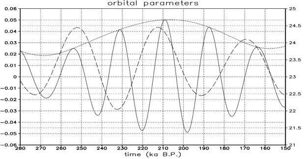
The 280–150 kyr BP interval was selected because it contains an eccentricity cycle with a large amplitude (although it is not the most extreme eccentricity cycle of the last 1 million years) and the most extreme obliquity oscillations of the last 1 million years.

All experiments described above have been carried out with the coupled atmosphere-ocean model and with the atmosphere-ocean-vegetation model. In the

10

simulations with the atmosphere-ocean model the vegetation was prescribed accord-ing to observed present day coverage and was kept constant duraccord-ing the simulations. The results of the simulations with the atmosphere-ocean-vegetation model will be denoted as PV, TV and PTV for the precession, obliquity and combined simulations, respectively (Table1).

15

For all simulations the boundary conditions like orography, land-sea configuration, ice sheets and concentration of trace gasses were kept constant. For the initial state present day conditions were used for all simulations. The results will be shown as averages over 100 years as the periods of the oscillations of the orbital parameters are much larger than 100 years.

20

3 Results

3.1 The African and Asian monsoon

In Tuenter et al. (2005) the African and Asian monsoon were combined because at Milankovitch timescales they behave similarly. However, it will become clear that at sub-Milankovitch timescales they behave differently and for that reason they will be

25

(9)

at-CPD

Printer-friendly Version Interactive Discussion mospheric sector 2 and latitudes 10◦N–20◦N while the Asian monsoon is the gridbox

located in atmospheric sector 3 and latitudes 20◦N–30◦N (Fig.1). At low latitudes the precession signal is much stronger than the obliquity signal, although the obliquity sig-nal is not negligible (Tuenter et al.,2005). Consequently, to a large extent experiments PT and PTV show the same characteristics as experiments P and PV, respectively.

5

Therefore we will focus on the results of experiments P and PV.

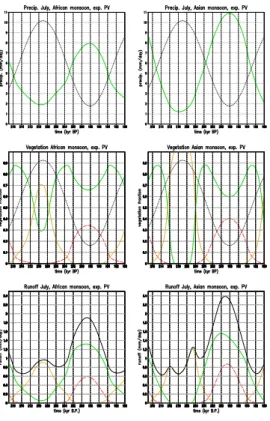
The monsoonal precipitation is stronger during minimum precession compared to maximum precession (Fig.3) which can be mainly attributed to the enhanced di fferen-tial heating between land and ocean due to the stronger insolation in boreal summer. Including an interactive vegetation model leads to a stronger response for both the

10

African and the Asian monsoon. This can be explained by a stronger hydrological cy-cle and larger albedo differences induced by vegetation (Brostr ¨om et al.,1998;Doherty et al.,2000;Tuenter et al.,2005).

The qualitative vegetation response to the precession forcing is similar for the African and Asian monsoon (Fig. 3). During precession minima the tree fraction increases

15

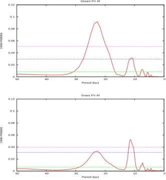
while during precession maxima the desert fraction increases. This can be attributed to the stronger monsoonal rainfall during precession minima compared to precession maxima. The increase of the desert fraction during precession maxima leads to the occurrence of sub-Milankovitch periods next to the precession period (Fig. 4) which also applies to the tree fraction (not shown). However, these sub-Milankovitch signals

20

are caused by “clipping” (Hagelberg et al.,1994) that is introduced by the fact that the vegetation fractions cannot be negative. The sharp transitions caused by the clipping introduce energy into the power spectrum at the harmonic frequencies of precession (Fig.4). These harmonics are an artifact of clipping (Hagelberg et al.,1994). Due to the alternating increase of the desert and tree fractions the grass fraction decreases both

25

during precession minima and maxima (Fig.3). This results in an additional period of about 10 kyr (or a half-precessional period) for the grass fraction, next to the (weaker) precession period (Fig. 4). The amplitude of the vegetation response to precession is larger for the Asian monsoon then for the African monsoon, especially during

(10)

pre-CPD

EGU cession maxima (Fig.3). When eccentricity is high, the entire Asian monsoon region

is even completely covered by desert during precession maxima. The larger desert fraction for the Asian monsoon compared to the African monsoon can be explained by the smaller amount of precipitation during precession maxima (Fig.3) and by the lower annual surface air temperature (not shown) for the Asian monsoon compared to the

5

African monsoon.

During precession minima the runoff from the African and Asian monsoon is largest in both experiment P and PV which is caused by the maximum precipitation (Fig.3). In experiment P the runoff is at a minimum during precession maxima which is in agree-ment with the minimum precipitation. This results in a precession period with no other

10

periods in the power spectrum of the runoff from experiment P (not shown). In exper-iment PV the runoff from the African monsoon is at a (secondary) maximum during precession maxima (Fig.3). These secondary maxima cause an additional 10 kyr pe-riod next to the precession pepe-riod (Fig.5). The runoff of the Asian monsoon is also at a maximum during weak precession maxima (i.e., around 255 and 163 kyr BP) in

experi-15

ment PV. However, during strong precession maxima the Asian monsoonal runoff is at a minimum and several thousands of years before and after this minimum the runoff is at a maximum (Fig.3). This leads to a weak (but significant) ∼5 kyr period next to the ∼10 kyr and the precessional period in the runoff signal for the Asian monsoon (Fig.5). To explain the mechanism underlying the occurrence of the sub-Milankovitch

variabil-20

ity in the runoff, we will focus on the period with the strongest minimum and maximum precession, i.e., 217–190 kyr BP. The periodic behaviour of the runoff is similar in all monsoon months but the largest amplitude occurs in July. For this reason we will only show the results for July.

Starting with a minimum precession (at 220 kyr BP, Fig.3) the total runoff from the

25

African monsoon decreases due to a decrease in the precipitation (Fig. 6). Due to this decrease of the precipitation the desert area grows at the expense of the grass fraction. This causes an increase of the total runoff (despite the decreasing precip-itation) because bare soil can hold less water than grass. At maximum precession

(11)

CPD

Printer-friendly Version Interactive Discussion (209 kyr BP) a secondary maximum in the runoff occurs due to the maximum extent

of the desert (Fig.6). After maximum precession the precipitation increases causing a decrease in the desert fraction and an increase in the grass fraction. This causes a de-crease in the runoff because the expanding grass fraction can hold more ground water. However, when precipitation further increases the runoff from the grass increases and

5

together with the runoff from the trees this leads to a runoff maximum around minimum precession at 198 kyr BP (Fig.6).

A similar explanation as given for the African monsoon also applies to the Asian mon-soon. As for the African monsoon the runoff increases around 213 kyr BP but now the desert fraction reaches its maximum while the precipitation is still decreasing (Fig.6).

10

This leads to a minimum runoff concurrent with the minimum precipitation at maximum precession (at ∼209 kyr BP). After maximum precession the runoff increases together with the increasing precipitation until around 206.5 kyr BP. After that the grass fraction starts to increase at the expense of desert area. This leads to a decrease of the runoff due to the stronger water holding capability of grass compared to desert. Finally, due

15

to the still increasing precipitation the runoff increases leading to a maximum around minimum precession (198 kyr BP).

In the obliquity experiment TV also no sub-Milankovitch variability occurs in the mon-soonal precipitation. In the vegetation fraction for the African and the Asian monsoon the sub-Milankovitch variability is similar as in experiment PV, i.e., the grass fraction

20

decreases due to an alternating increase in the desert fraction and in the tree fraction (not shown). This leads to a period of about 20 kyr next to the period of 41 kyr. How-ever, the amplitudes of the variations in the vegetation fractions are small in experiment TV, i.e., changes of about 0.1. There is no sub-Milankovitch variability in the runoff for both the African and Asian monsoon in experiment TV. This is because the vegetation

25

variations are too small to induce sub-Milankovitch variability in the runoff.

The results of the combined experiment PTV are almost linear combinations of the results of experiments PV and TV (Tuenter et al.,2005). This means that the vegeta-tion and runoff for the African and Asian monsoon in experiment PTV is governed by

(12)

CPD

EGU experiment PV due to the small amplitude of experiment TV. This leads to similar

sub-Milankovitch variability in the vegetation and runoff as shown in Fig. 3 in experiment PTV.

3.2 Sub-Milankovitch in other regions

Similar sub-Milankovitch variability in the vegetation as shown in Fig.3also exists for

5

high- and mid-latitudinal regions for both obliquity and precession. Some examples are the northern Asian continent (Fig.7), northern Canada (atmospheric sector 7, 60◦N– 70◦N, not shown) in experiments PV and TV and the East Asian region (atmospheric sector 4, 30◦N–40◦N) in experiment PV (not shown). For obliquity this introduces a sub-Milankovitch period of about 20 kyr which is very close to the primary orbital

10

periods of precession (19 and 23 kyr).

An example for which sub-Milankovitch variability in the vegetation does not only introduce sub-Milankovitch variability in the runoff, but also in the Surface Air Tem-perature (SAT) is given for the Sahara (Fig. 7). The secondary maxima and minima in the Saharan SAT are caused by albedo changes induced by vegetation changes.

15

This example also shows that secondary minima/maxima in a climate parameter can occur during precession minima as well as during precession maxima as found for the monsoonal runoff. Sub-Milankovitch variability in other climatic parameters (both in the ocean and atmosphere) are also found. However, this variability is either very small or it is caused by clipping (Crowley et al.,1992;Hagelberg et al.,1994), e.g. for

20

snow fractions (Fig.7) and sea-ice fractions (not shown). This clipping introduces arti-ficial sub-Milankovitch variability at the harmonic frequencies of precession (Hagelberg et al.,1994). Furthermore, it also transports energy into the power spectrum at the modulating period of precession, i.e. eccentricity (Crowley et al.,1992).

(13)

CPD

4 Summary and discussion

In this study, we investigated whether climate variability at sub-Milankovitch periods (>2 kyr and <15 kyr) can be simulated in long (130 kyr) experiments with an EMIC (Climber-2). Our approach was to study the climate response to the separate obliquity and precession forcing. Furthermore, we also performed the simulations with and

5

without an interactive vegetation model.

For the strength of the African and Asian monsoon no sub-Milankovitch variability was found in any simulations. However, in the precession experiment with interactive vegetation sub-Milankovitch variability in the vegetation and runoff in the monsoonal regions is simulated. In the run with constant vegetation no sub-Milankovitch periods

10

in the monsoonal runoff were found. The mechanism for sub-Milankovitch signals in the vegetation is similar for the Asian and African monsoon regions: The grass fraction decreases due to the increase of both the desert fraction (during maximum precession) and the tree fraction (during minimum precession). This introduces a sub-Milankovitch period of about 10 kyr for the grass fraction. The sub-Milankovitch signal in the

mon-15

soonal runoff is caused by the different water holding capacity of trees, grass and desert. The sub-Milankovitch period of the African monsoon (only ∼10 kyr) differs from the Asian monsoon (∼10 kyr and ∼5 kyr) due to differences in the amplitudes of the vegetation signal.

The mechanism for sub-Milankovitch variability in the vegetation at low latitudes can

20

be also found at high and mid-latitudes. At high latitudes this is also possible for obliq-uity leading to an additional period of ∼20 kyr which is close to the primary orbital peri-ods of precession. With an example of the Sahara it was shown that sub-Milankovitch variability in vegetation can not only induce sub-Milankovitch variability in runoff but also in surface air temperature due to albedo changes. Finally, other examples of

sub-25

Milankovitch variability were found but they were either small or they were caused by clipping which causes artificial sub-Milankovitch periods (Hagelberg et al.,1994).

(14)

CPD

EGU fact that the desert fully covers the entire Asian monsoon region during strong

preces-sion maxima while it only partly covers the African monsoon region (Fig.3). This can be explained by the smaller amount of annual precipitation and the lower annual tem-perature during precession maxima for the Asian monsoon compared to the African monsoon. However, they strongly depend on the background climate which is mainly

5

governed by the chosen value of obliquity (here 22.08 degrees), the atmospheric com-position (pre-industrial values for carbon dioxide and methane) and the size of the ice sheets (present-day ice sheets). Changing these boundary conditions could easily in-duce other sub-Milankovitch variability, for instance a ∼5 kyr period in the runoff of the African monsoon and/or no ∼5 kyr period for the Asian monsoon runoff. Consequently,

10

the simulated sub-Milankovitch periods for the monsoonal runoff is only one possible realization. These periods depend on the background climate that changes when the boundary conditions change.

Including varying ice sheets is not necessary for simulating sub-Milankovitch vari-ability in our model. This is in agreement with Ortiz et al. (1999) who found

sub-15

Milankovitch variability in the Atlantic Ocean for the period prior to the onset of the glacial cycles at ∼2.8 million years BP. However, this does not imply that ice sheets cannot change the characteristics of sub-Milankovitch variability. For instance,Sun and Huang (2006) found a half-precession cycle in the loess-soil sequence of the last inter-glacial reflecting changes in the East Asian summer monsoon circulation. For the last

20

glacial they did not find sub-Milankovitch variability due to the reduced influence of the summer monsoon on their study area. Another example is the weak sub-Milankovitch variability in a dust record from the eastern Mediterranean Sea from 3 million years BP until the mid-Pleistocene transition (Larrasoa ˜na et al., 2003). During and after the mid-Pleistocene transition, when the amplitude of the Northern Hemisphere ice

25

sheets changes increase, the sub-Milankovitch variability gets much stronger. This suggests that the strength of sub-Milankovitch variability depends on the size of the ice sheets. Transient simulations with climate models including an interactive ice sheet model might show this influence of ice sheets on sub-Milankovitch variability.

(15)

CPD

Printer-friendly Version Interactive Discussion The sub-Milankovitch periods of about 10 and/or 5 kyr in the Asian and African region

are in agreement with proxy-based evidence. Sun and Huang (2006) suggest that their periods in the northwestern Chinese Loess Plateau originate from half-precession cycles in the insolation from low latitudes. Our results suggest that their signal could also reflect local sub-Milankovitch periods in vegetation and/or runoff.

5

Comparing the sub-Milankovitch variability from this study to marine signals is not possible in a direct way, because Climber-2 includes a coarse zonally averaged ocean model. This hinders the research of the influence of the monsoonal runoff on the At-lantic and Indian Ocean. Sub-Milankovitch periods of ∼10 kyr and/or ∼5 kyr periods are also found in marine records both in the Atlantic Ocean (Pokras and Mix,1987;

Hagel-10

berg et al.,1994;McIntyre and Molfino,1996), in the Mediterranean Sea (Larrasoa ˜na et al.,2003;Becker et al.,2005) and in the Indian Ocean (Pestiaux et al.,1988;Naidu, 1998). In general, these authors explain their signals by variations in the strength of the monsoon. Our results suggest that the signals can be explained by variations in the monsoonal runoff rather than variations in the strength of the monsoon. The changing

15

runoff induces variations in the salinity of the ocean which could cause a signal by itself or through salinity induced circulation changes.

Acknowledgement. This work was supported by the Netherlands Organization for Scientific

Research (NWO) under a VIDI grant to L. J. Lourens.

References

20

Becker, J., Lourens, L. J., van der Laan, F. J., Kouwenhoven, T. J., and Reichart, G. J.: Late pliocene climate variability on Milankovitch to millennial time scales: A high-resolution study of MIS100 from the Mediterranean., Palaeogeography, Palaeoclimatology, Palaeoecology, 228 , 338–360, 2005. 746,758

Berger, A. L.: Long-term variations of daily insolation and Quaternary climatic changes, Journal

25

of the Atmospheric Sciences, 35, 2362–2367, 1978. 750

Brovkin, V., Ganopolski, A., and Svirezhev Y.: A continuous climate-vegetation classification for use in climate-biosphere studies, Ecol. Modell., 101, 251–26, 1997.

(16)

CPD

EGU

Brostr ¨om, A., Coe, M., Harrison, S. P., Gallimore, R., Kutzbach, J. E., Foley, J., Prentice, I. C., and Behling, P.: Land surface feedbacks and palaeomonsoons in northern Africa, Geophys. Res. Lett., 25 , 3615–3618, 1998. 752

Claussen, M., Kubatzki, C., Brovkin, V., and Ganopolski, A.: Simulation of an abrupt change in Saharan vegetation in the mid-Holocene, Geophys. Res. Lett., 26 , 2037–2040, 1999. 750

5

Claussen, M., Mysak, L. A., Weaver, A. J., Crucifix, M., Fichefet, T., Loutre, M.-F., Weber, S. L., Alcamo, J., Alexeev, V. A., Berger, A., Calov, R., Ganopolski, A., Goosse, H., Lohmann, G., Lunkeit, F., Mokhov, I. I., Petoukhov, V., Stone, P., and Wang, Z.: Earth system models of intermediate complexity: closing the gap in the spectrum of climate system models, Climate Dyn., 18, 579–586, 2002. 748

10

Crowley, T. J., Kim, K.-Y., Mengel, J. G., and Short, D. A.: Modeling the 100,000-Year Climate Fluctuations in Pre-Pleistocene Time Series, Science, 255, 705–707, 1992. 748,755

Doherty, R., Kutzbach, J., Foley, J., and Pollard, D.: Fully coupled climate/dynamical vegetation model simulations over Northern Africa during the mid-Holocene, Climate Dyn., 16, 561– 573, 2000. 752

15

Ganopolski, A., Kubatzki, C., Claussen, M., Brovkin, V., and Petoukhov, V.: The influence of vegetation-atmosphere-ocean interaction on climate during the mid-Holocene, Science, 280, 1916–1919, 1998a. 750

Ganopolski, A., Rahmstorf, S., Petoukhov, V., and Claussen, M.: Simulation of modern and glacial climates with a coupled global model of intermediate complexity, Nature, 391, 351–

20

356, 1998b. 750

Ganopolski, A., Petoukhov, V., Rahmstorf, S., Brovkin, V., Claussen, M., Eliseev, A., and Ku-batzki, C.: CLIMBER-2: a climate system model of intermediate complexity. Part II: model sensitivity, Climate Dyn., 17, 735–751, 2001. 750

Hagelberg, T. K., Bond, G., and deMenocal, P.: Milankovitch band forcing of sub-Milankovitch

25

climate variability during the Pleistocene, Paleoceanography, 9 , 545–558, 1994. 746,747,

748,752,755,756,758

Heslop, D. and Dekkers, M. J.: Spectral analysis of unevenly spaced climatic time series using CLEAN: signal recovery and derivation of significance levels using a Monte Carlo simulation, Phys. Earth Planet. Interiors, 130, 103–116, 2002. 766,767

30

Imbrie, J., Boyle, E. A., Clemens, S. C., Duffy, A., Howard, W. R., Kukla, G., Kutzbach, J. D., Martinsson, G., McIntyre, A., Mix, A. C., Molfino, B., Morley, J. J., Peterson, L. C., Pisias, N. G., Prell, W. L., Raymo, M. E., Shackleton, N. J., and Toggweiler, J. R.: On the structure and

(17)

CPD

origin of major glaciation cycles 1. Linear responses to Milankovitch forcing, Paleoceanogra-phy, 7 , 701–738, 1992. 747

Jackson, C. S. and Broccoli, A. J.: Orbital forcing of Arctic climate: mechanisms of cli-mate response and implications for continental glaciation, Clicli-mate Dyn., 21, 539–557, doi:10.1007/s00382-003-0351-3, 2003. 747

5

Kubatzki, C., Montoya, M., Rahmstorf, S., Ganopolski, A., and Claussen, M.: Comparison of the last interglacial climate simulated by a coupled global model of intermediate complexity and an AOGCM, Climate Dyn., 16, 799–814, 2000. 750

Larrasoa ˜na, J. C., Roberts, A. P., Rohling, E. J., Winkelhofer, M., and Wehausen, R.: Three million years of monsoon variability over the northern Sahara, Climate Dyn., 21, 689–698,

10

doi:10.1007/s00382-003-0355-z, 2003. 746,748,757,758

Le Treut, H. and Ghil, M.: Orbital forcing, climatic interactions, and glaciation cycles, J. Geo-phys. Res., 88 , 5167–5190, 1983. 747

McIntyre, A. and Molfino, B.: Forcing of Atlantic equatorial and subpolar millenial cycles by precession, Science, 274, 1867–1870, 1996. 746,747,748,758

15

Naidu, P. D.: Driving forces of Indian summer monsoon on Milankovitch and sub-Milankovitch time scales: A review, J. Geol. Soc. India, 52, 257–272, 1998. 747,758

Ortiz, J., Mix, A., Harris, S., and O’Connell, S.: Diffuse spectral reflectance as a proxy for percent carbonate content in North Atlantic sediments, Paleoceanography, 14 , 171–186, doi:10.1029/1998PA900021, 1999. 747,757

20

Pestiaux, P., van der Mersch, I., and Berger, A.: Paleoclimate variability at frequencies ranging from 1 cycle per 10 000 years to 1 cycle per 1000 years: Evidence for nonlinear behaviour of the climate system, Climatic Change, 12, 9–37, 1988. 747,748,758

Petoukhov, V., Ganopolski, A., Brovkin, V., Claussen, M., Eliseev, A., Kubatzki, C., and Rahm-storf, S.: CLIMBER-2: a climate system model of intermediate complexity. Part I: model

25

description and performance for present climate, Climate Dyn., 16, 1–17, 2000. 749,750

Pokras, E. M. and Mix, A. C.: Earth’s precession cycle and Quaternary climatic change in tropical Africa, Nature, 326, 486–487, 1987. 746,747,748,758

Roberts, D. H., Lehar, J., and Dreher, J. W.: ime-Series Analysis with Clean. 1. Derivation of A Spectrum, Astronomical J., 93, 968–989, 1987. 766,767

30

Rodr´ıguez-Tovar, F. J. and Pardo-Ig´uzquiza, E.: Strong evidence of high-frequency (sub-Milankovitch) orbital forcing by amplitude modulation of Milankovitch signals, Earth Planet. Sci. Lett., 210, 179–189, doi:10.1016/S0012-821X(03)00131-6, 2003. 746,747

(18)

CPD

EGU

Saltzman, B. and Sutera, A.: A model of the internal feedback system involved in late Quater-nary climatic variations, J. Atmos. Sci., 41 , 736–745, 1984. 747

Short, D. A., Mengel, J. G., Crowley, T. J., Hyde, W. T., and North, G. R.: Filtering of Milankovitch cycles by Earth’s geography, Quaternary Res., 35, 157–173, 1991. 747,748

Steenbrink, J., Kloosterboer-van Hoeve, M. L., and Hilgen, F. J.: Millennial-scale climate

varia-5

tions recorded in Early Pliocene colour reflectance time series from the lacustrine Ptolemais Basin (NW Greece), Global Planet. Change, 36, 47–75, 2003. 746

Stocker, T. F., Wright, D. G., and Mysak, L. A.: A zonally averaged coupled ocean-atmosphere for paleoclimate studies, J. Climate, 5, 773–797, 1992. 749

Sun, J. and Huang, X.: Half-precessional cycles recorded in Chines loess: response to

low-10

latitude insolation forcing during the last interglaciation, Quaternary Sci. Rev., 25, 1065– 1072, 2006. 757,758

Tuenter, E., Weber, S. L., Hilgen, F. J., and Lourens, L. J.: The response of the African summer monsoon to remote and local forcing due to precession and obliquity, Global Planet. Change, 36, 219–235, 2003. 750,751

15

Tuenter, E., Weber, S. L., Hilgen, F. J., Lourens, L. J., and Ganopolski, A.: Simulation of climate phase lags in the response to precession and obliquity forcing and the role of vegetation, Climate Dyn., 24, 279–295, doi:10.1007/s00382-004-0490-1, 2005. 748, 751, 752, 754,

(19)

CPD

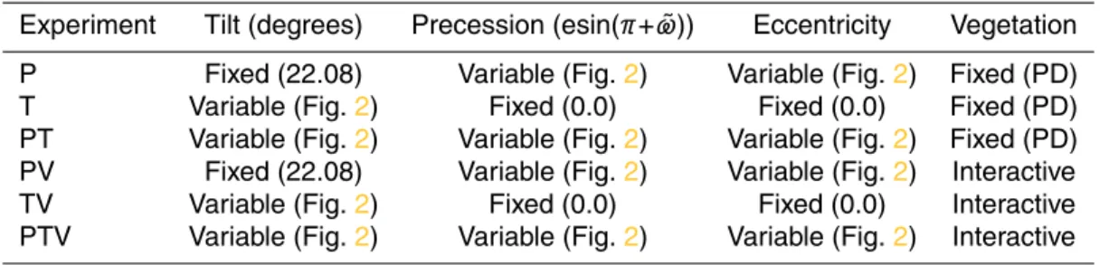
Table 1. Orbital configuration and vegetation used for the 6 transient experiments as described

inTuenter et al.(2005). P is the precession experiment with fixed vegetation, T is the obliq-uity (Tilt) experiment with fixedvegetation and PT is the combined precession and obliqobliq-uity experiment with fixed vegetation. PV, TV, and PTV are the precession, obliquity and combined experiments with interactive vegetation, respectively. PD stands for Present Day. The tilt is defined as the angle between the ecliptic and the equator, e is the eccentricity of the orbit of the Earth and ˜ω is the angle between the vernal equinox and perihelion (measured counter

clockwise).

Experiment Tilt (degrees) Precession (esin(π+ ˜ω)) Eccentricity Vegetation P Fixed (22.08) Variable (Fig.2) Variable (Fig.2) Fixed (PD) T Variable (Fig.2) Fixed (0.0) Fixed (0.0) Fixed (PD) PT Variable (Fig.2) Variable (Fig.2) Variable (Fig.2) Fixed (PD) PV Fixed (22.08) Variable (Fig.2) Variable (Fig.2) Interactive TV Variable (Fig.2) Fixed (0.0) Fixed (0.0) Interactive PTV Variable (Fig.2) Variable (Fig.2) Variable (Fig.2) Interactive

(20)

CPD

EGU

Fig. 1. Representation of the Earth geography in CLIMBER-2.3. Horizontal dashed lines

sep-arate grid cells for the atmospheric grid (the latitudinal resolution for the ocean is 2.5◦). Vertical dashed lines show only atmospheric grid cells. Atmospheric sectors are numbered in the cir-cles. Black area indicates only the relative fractions of land and ocean in the atmospheric grid cells. Solid vertical lines show the partition between the three ocean basins.

(21)

CPD

Fig. 2. Orbital parameters for the period 280–150 ka BP: Eccentricity (short dashed), the

pre-cession parameter (solid) and obliquity (long dashed). The left vertical axis displays the values for eccentricity and the precession parameter. The right axis shows the values for obliquity (in degrees). The horizontal axis displays time (in 1000 years Before Present).

(22)

CPD

EGU

Fig. 3. Precipitation (top panels) and runoff (bottom panels) averaged for June-September for

experiment PV (thick green line) and experiment P (thin blue line). Middle panels: Annual grass fraction (thick green line), annual tree fraction (dashed red line) and annual desert fraction (thin, dark yellow line) for experiment PV. The left panels are results for the African monsoon and the right panels for the Asian monsoon. In all panels the precession parameter is plotted (dotted line, arbitrary scale). The horizontal axes denote time in 1000 years Before Present).

(23)

CPD

Printer-friendly Version Interactive Discussion 0 0.02 0.04 0.06 0.08 0.1 0.12 0 10 20 30 40 50 Clean-modulus Period (kyr) Desert PV Af 0 0.02 0.04 0.06 0.08 0.1 0.12 0 10 20 30 40 50 Clean-modulus Period (kyr) Grass PV Af

Fig. 4. Power spectrum of results from experiment PV for the desert fraction (upper panel) and

the grass fraction (lower panel) for the African monsoon. The pink, blue and green line indicate the 99.5%, 99% and 95% confidence level, respectively. Power spectra were obtained by using the CLEAN transformation ofRoberts et al.(1987). For the determination of significance levels associated with the frequency spectra of the CLEAN algorithm, we applied a Monte Carlo based method developed byHeslop and Dekkers(2002), which was run as a MATLAB routine. The CLEAN spectra were determined by adding 10% red noise (i.e., control parameter= 0.1), a clean/gain factor of 0.1, 500 CLEAN Iterations, an interpolation step (dt) value of 100 year, and 1000 simulation iterations.

(24)

CPD

EGU

Fig. 5. Power spectra of results from experiment PV for the June-September runoff for the

African monsoon (upper panel) and for the Asian monsoon (lower panel). Power spectra were obtained by using the CLEAN transformation ofRoberts et al.(1987). For the determination of significance levels associated with the frequency spectra of the CLEAN algorithm, we applied a Monte Carlo based method developed byHeslop and Dekkers (2002), which was run as a MATLAB routine. The CLEAN spectra were determined by adding 10% red noise (i.e., control parameter= 0.1), a clean/gain factor of 0.1, 500 CLEAN Iterations, an interpolation step (dt) value of 100 year, and 1000 simulation iterations.

(25)

CPD

Fig. 6. Top panels: Precipitation for July (solid green line) and the precession parameter (dotted

line, arbitrary scale). Middle panels: Annual grass fraction (thick green line), annual tree fraction (dashed red line) and annual desert fraction (thin, dark yellow line) for experiment PV. Bottom panels: Total runoff (thick black line), runoff originating from the grass area (thick green line), from the tree area (dashed red line) and from the desert area (thin, dark yellow line), all for July. All results are from experiment PV and the pictures on the left side are results for the African monsoon and on the right side for the Asian monsoon. The horizontal axes denote time in 1000 years Before Present).

(26)

CPD

EGU

Fig. 7. Top panels: Annual grass fraction (thick green line), annual tree fraction (dashed red

line) and the annual desert fraction ( thin, dark yellow line) for northern Russia (atmospheric sector 3, 70◦N–80◦N) for experiment PV (left panel) and experiment TV (right panel). Bottom left panel: Snow fraction averaged over June-July-August for Siberia (atmospheric sector 4, 60◦N–70◦N) for experiment PV (thick green line) and experiment P (thin blue line). Bottom right panel: Anomalous runoff averaged over June-July-August (thick green line) and anoma-lous surface air temperature averaged over December-January-February (dashed red line) for the Sahara (atmospheric sector 2, 20◦N–30◦N) and for experiment PV. In all panels the pre-cession parameter is plotted (dotted line, arbitrary scale) except for the top right panel where the obliquity parameter is plotted (dotted line, arbitrary scale). The horizontal axes denote time in 1000 years Before Present).