Diagnostic study on the forcing of the Ferrel cell

by

GIOVANNA SALUSTRI

Laurea in Fisica, University of Bologna (1974)

SUBMITTED TO THE DEPARTMENT OF METEOROLOGY AND PHYSICAL OCEANOGRAPHY

IN PARTIAL FULFILLMENT OF THE

REQUIREMENTS FOR THE DEGREE OF

MASTER OF SCIENCE IN

METEOROLOGY

at the

MASSACHUSETTS INSTITUTE OF TECHNOLOGY

June 1982

(

Massachusetts Institute 'of Technology 1982

Signature of Author

Certified by

Accepted by

Department of Meteorology and Physical Oceanography May 7, 1982

Peter H. Stone Thesis Supervisor

Ronald G. Prinn Chairman, Departmental Graduate Committee

Undgjren

U n

jS

1982

DIAGNOSTIC STUDY ON THE FORCING OF THE FERREL CELL

by

GIOVANNA SALUSTRI

Submitted to the Department of Meteorology and Physical Oceanography on May 7, 1982 in partial fulfillment of the requirements

for the Degree of Master of Science in Meteorology

ABSTRACT

A diagnostic study of the relative importance of the

eddy transport of sensible heat, latent heat and zonal momentum, for the forcing of the Ferrel cell in the Northern Hemisphere is carried out, using Oort and Rasmusson's data set. The nonhomogeneous second-order paitial differential

equation for the vertical p-velocity CA , obtained from the

quasi-geostrophic vorticity and thermodynamic equations, is used. This equation is zonally averaged and solved by finite difference methods. The contribution of humidity is introduced, so the dry static stability is replaced by a measure of the moist static stability, and the forcing of the Ferrel cell by eddy latent heat fluxes as well as sensible heat and momentum fluxes is included. A variable

Coriolis parameter, f(y ), is considered.

The results concerning the general structure, strength and location of the Ferrel cell forced by the eddy fluxes are in good agreement with those of previous studies. However differences are found in the contributions of the

three different forcing functions to the solution: the contributions are comparable in magnitude, with the latent heat forcing being slightly smaller than the others. In previous studies, the contribution due to the eddy transport of zonal momentum seemed to be about twice that due to the eddy transport of sensible heat, and the contribution due to the eddy transport of latent heat was neglected.

Thesis Supervisor Dr. Peter H. Stone

Table of contents. Page 1. Intr oduction ... 4 2. Governing equations ... ₇ 3. Observational data ... 15 4. Method of solution ... 16

5. Annual mean results .... ... 21

6. Comparisons with other studies ... 27

7. Seasonal results ... ... 35

Acknowledgments ... 38

R efer en ces . ... 39

Table caption s ... 42 T a b le s ... .... .... .... ... ... ... ... ... .... ... ... 4 5

1. Introduction.

Diagnostic studies of the mean meridional circulation _{have been carried out by Kuo (1956), Holopainen}

(1967), Vernekar (1967) and others. Kuo pointed out that

the _{mean meridional circulation is forced by the zonal mean} eddy transports of heat and momentum, by the diabatic heating _{and by the frictional dissipation and evaluated the} mean meridional circulation. Holopainen estimated the strength of this circulation required to balance the angular momentum in a steady state. Vernekar, using the quasi-geostrophic C3 equation, computed the mean meridional circulation forced by given eddy transports of heat and momentum; he used monthly mean data, taken from Wiin-Nielsen, Brown and Drake (1963,1964), for January, April, July, October 1962, January 1963 and January 1964 at five, sometimes eight isobaric levels, from 20'N to 87.5*ON,

for each 2.5* of latitude.

The present study is in principle similar to Kuo's and Vernekar's, but uses a better set of data: those by Oort and Rasmusson (1971), which constitute a large, homogeneous set; these data were collected from about 700 hemispheric and equatorial stations for the five year period₁ May 1958 through April 1963. The data elaborated by Oort and Rasmusson are zonally averaged and available at eleven isobaric levels, from the Equator to 750N, each 5* of

latitude.

The main purpose of this paper and its most important difference from previous studies is the inclusion of latent heat effects in the calculation; we intend to study how the Ferrel mean meridional circulation is forced

by latent heat, sensible heat and momentum eddy transport, in the annual mean and extreme seasons.

Qualitatively from the data of Oort and Rasmusson, it can be seen that the heating due to the convergence of sensible heat and latent heat are of the same order in the region of the Ferrel cell. The latter is smaller than the former and almost in phase, even if not quite: because of the presence of a larger amount of moisture in low latitudes, the maximum of the latent heat eddy flux is nearer the Equator than that of the sensible heat eddy flux. Besides, due to the presence of the latent heat eddy fluxes,

the dry static stability is replaced by the smaller6 (j,p),

measure of the moist static stability in presence of saturated air, and this implies a stronger response of the system to our forcings. A Coriolis parameter, also variable

with latitude, is used in the present study.

The data of the meridional eddy transfers of

sensible heat, latent heat and momentum, in which we are interested, are very good and reliable. In the present study, the zonally averaged quasi-geostrophic W equation

(Lorenz, 1967) is used; this equation shows how the mean meridional circulation is forced by eddy transfer of zonal momentum, eddy transfer of sensible heat, friction forces and diabatic heating. The contributions to the forcing function by friction forces and diabatic heating, due to radiation and small scale convection, are neglected, because the direct or indirect methods of evaluating them are not accurate enough.

Due to the linearity of the problem, the contributions to the zonally averaged p-vertical velocity EL0J by the considered forcing terms are studied separately and then added; the annual and seasonal results obtained for the partial and total solutions E.) are finally discussed and compared with results of previous papers. The present study is a continuation of two previous papers (Salustri, 1981, 1982), in which a preliminary study on the contributions of sensible heat, latent heat and momentum forcings on the solution was performed.

2. Governing equations.

In the present paper the Ferrel cell's mean meridional circulation is assumed to be governed by the quasi-geostrophic equations; a variable Coriolis parameter,

f(T ), a function of latitude, is considered and the friction effects are neglected; under these assumptions, the vorticity equation can be written as follows:

- - ). (2.1)

where is the geostrophic vorticity, p is the pressure,

W =

dp/dt

is the vertical velocity in p coordinates, U is the geostrophic wind and V indicates the horizontal divergence. From the geostrophic relations it follows that

0, and that the vorticity can be expressed as S

7T

, where is the geopotential; hence the vorticity equation (2.1) can be rewritten as:

[B{~

4)1(2.2)

In order to get an equation for the vertical velocity

()

the following thermodynamic equation will be considered together with the above-written vorticity

equation:

+-U (2.3)

where = - - K- is a measure of the dry static

stability with K =

R

, and C? are approximated by the gas constant for dry air and the specific heat at constant pressure for dry air, respectively,

T

is the temperature, subscript s indicates its basic vertical profile and

Q

is the net heating per unit mass; the main contributions to

Q

are from latent heatQL , and

radiations , where:

Lv

is the latent heat of condensation,

9

is the specific humidity, and

V

is the horizontal wind (geostrophic and ageostrophic). Substituting

where

9.

and

9

are respectively the specific humidity basic vertical profile and fluctuation, /. is the longitude

and

(f

is the latitude, by using the continuity equation,

Q

can be rewritten as:

where

U'

is the horizontal ageostrophic wind.

In the assumptions of the quasi-geostrophic theory, we can neglect the humidity ageostrophic

\((() , and the term including the

convection,

2

(c

)

.

In

addition, af

applied the zonal average to our equations, humidity meridional advection by the

velocity,

[\\/.\7c

S , can be also neglected; are smaller than the humidity geostrophic

\7

(V

1) , by a factor of order the

Moreover, the radiative heating will not

horizontal flux, vertical moist ter we shall have the mean zonal mean meridional all these terms horizontal flux, Rossby number. be studied in the present paper; forcings. Hence rewritten as:

this does not affect the study of the other

the thermodynamic equation (2.3) can be

---

+

U-\

^

L

W

\)

(2.4)

-RLV D95

where 6and, substituting the expression for

C-the dry static stability and using the hydrostatic and the ideal gas state equations in order to relate the temperature and the geopotential fields, 6 can be rewritten as it

follows:

which is a measure of the moist static stability in presence of saturated air. The relative humidity, obtained from the data used in the present study, does not show any saturated region, hence 6 can not be interpreted 'as the moist static stability; this agrees with the fact that 6 can even assume negative values, which is discussed below in Section 4. The function

G

and the dry static stability 6 , as computed from Oort and Rasmusson's data, zonally averaged and time averaged over the five year period May 1958 through April 1963, are shown in the gridpoints for which the North

Hemisphere's data are available, as functions of latitude and pressure, in Tables 1 and 2 respectively. The two quantities are both given in the units m' s- mb. In previous papers, like those by Wiin-Nielsen (1959) and

Vernekar (1967), the dry static stability is approximated as

a function of p, ~ * 2 with constant

G,

; in the present study, having introduced the contribution of the specific humidity, ) will not be approximated in a similar

way, because the latitudinal fluctuations of 6 are larger than those of the dry static stability

6"

; this can be seen from a comparison between Table I and Table 2. Thus a

6' , function both of latitude and pressure, is considered here.

If we take the p-derivative of the vorticity equation (2.2) and the Laplacian of the thermodynamic equation (2.4) and subtract, the time derivatives are eliminated and we get the t) -equation:

< (2.5)

IP

CF

The time variations of

9

can be neglected with respect to the

9

-advection in equation (2.5), if we consider time averages longer than or of the order of one month or if we consider extreme seasons. In the present study, we use data averaged over a five year period and, in the final section, data for the extreme seasons from the same period. Thus we introduce the time average

(

=

(-t,)'(

)dt

,

where

t, and

t2 are specified in

Section 3 for the annual problem and in Section 7 for the seasonal one, and we rewrite the (.. -equation as follows:

\~/

)\\/+

\[(CLv~

(2.6)

Introducing the polar coordinates ( ,

defining the zonal average E( )3 = ( )-f and applying this operation to (2.6), this last equation can be rewritten in the following way:

"

,

-

(,(2.7)

cD os 0

where

where ' is the radius of the earth, E/V3 is the northward transport of westerly momentum by transient eddies plus stationary eddies, E T v 3 is the northward transport of sensible heat by transient eddies plus stationary eddies. In addition, the latent heat eddy flux is present in

Eq. (2.7): E9v 3 is the northward transport of water vapor

by transient eddies plus stationary eddies. More will be

said about the data used in Section 3.

temperature, specific humidity and geopotential do not appear because of our use of the quasi-geostrophic hypotheses. They are not known very well in any case.

The forcing function M(L?) consists of two contributions; the former Ml(?,p) is related to the vertical variation of eddy transfer of zonal momentum, the latter contains two termsrelated to the horizontal variation of eddy transfers of sensible heat and latent heat, respectively. The contributions to the forcing function deriving from the vertical variation of viscous forces and the horizontal variation of that portion of diabatic heating, due to radiation and small scale convection, are neglected, because the direct or indirect methods of evaluating them are not accurate enough.

Having considered a moist atmosphere in the present study, we find two new elements introduced in Eq. (2.7), with respect to the similar equations used in previous papers: the first, and more evident, is the latent heat forcing term; the second is the new function Gr which replaces the bigger stability parameter C and makes us expect a stronger response from the system, as will be shown below in Section 5.

Boundary conditions.

The differential equation for the vertical motion is solved by two different methods and boundary conditions. In the first case, the vertical motion is considered to be zero at the top and bottom extreme levels in which the data are available, i.e. p = 50 mb and p = 1000 mb, respectively; in the second, it is considered to be zero at the top and bottom of the positive 6' region. The vertical velocity at the bottom of the atmosphere due to sloping terrain is neglected. More will be said about these boundary conditions in Section 4.

As equatorial lateral boundary condition we assume a vertical velocity CW symmetrical with respect to the Equator, i.e. - = 0 as Vernekar does; this condition

is certainly proper for the study of the annual mean problem, and does not affect the mid-latitude seasonal results studied in the final section, as is implied by the sensitivity test discussed below in Section 5.

At the Pole, we also use the lateral boundary

3. Observational data.

The following data are used in the present study: the mean temperature ET 3, the mean specific humidity [q 3 and the mean geopotential height E4 3, necessary for obtaining the function ( and the northward transport of westerly momentum, sensible heat and water vapor by

transient eddies and standing eddies, (Eu,'v'3 + EUv2),

(IT'v'

3 + [TAvVJ), and (['v' 3 + [Cmv"J) respectively,

required for computing the forcing functions.

All these data are taken from Oort and Rasmusson's

"Atmospheric Circulation Statistics" (1971). The data used are zonally averaged and time averaged over the five year period May 1958 trough April 1963 and are available, for the Northern Hemisphere, from O0 _{to 75}0_{N , each 5*of latitude,}

and at eleven pressure levels: 50, 100, 200, 300, 400, 500, 700, 850, 900, 950, 1000 mb.

4. Method of solution.

In previous similar works by Vernekar (1967) and the author (1981 ), the W3 -equation is solved by developing

both the unknown )(?,p)] and the forcing function M(L4i) in Legendre polynomials in latitude, and then solving the resulting one dimensional equation for the vertical structure by ordinary centered finite difference methods and

by performing a Fourier analysis, respectively. In the present study, having considered a moist atmosphere and, as a consequence,6(kyr) being a function both of latitude and pressures the previous approaches are no longer suitable, and Eq. (2.7) is solved by finite difference method, both along the vertical and the horizontal, and the overelaxation method, with the relaxation parameter of =1.4 . Because of the particular grid for which the data by Dort and Rasmusson are available, second order schemes for nonequispaced data are used at the eleven pressure levels from p

=

50 mb to p = 1000 mb, along the vertical, while the same kind of schemes, but for equispaced data, are used at the sixteen latitudinal points from the Equator to 75* N ; the schemes used can be found in Hornbeck (1975). After performing finite differentiations on the eddy transport data, which is smooth in latitude and pressure, the resulting forcing

functions that we get appear to be smooth functions too and it is not necessary to apply any filter.

In dealing with Eq. (2.7) one difficulty arises from what we already pointed out in Section 2, that 6 assumes negative values in the southern and lower part of our domain. Because of this change of sign, the nature itself of Eq. (2.7) changes from an elliptic type, in the region where & is positive, to an hyperbolic one, where is negative. However, we are interested mainly in middle

latitudes for the study of the Ferrel cell, and besides the quasi--geostrophic equations do not hold any longer when the values of the vertical stability become too small, as happens in the regions where 6 is small or negative, hence we do not calculate the vertical velocity E633 in the negative 6 region, and only the elliptic equation is solved, by using two different methods. In the former, called "A Case" hereafter, one small positive constant value is arbitrarly assigned to V in the G negative region and a sensitivity test, run by changing the assigned positive

value several times, shows the solution E W3 3 is not

affected appreciably in the region where was originally positive.

Before going to describe the latter case, something will be said on the influence of the boundary conditions on the solution. If the real values of the mean vertical motion [W3 are supposed to be known at the boundaries,

[ = To at the top boundary (4.1)

[Co] [I3) at the bottom boundary (4.2)

due to the linearity of Eq. (2.7), the total solution, [(a3,

which results from the influence of the internal forcing and boundary conditions, can be written as the sum of three independent contributions:

[ W) = [W])I +[(W 3 T +EW33

where [C))W [I 3 and [W33 represent the mean vertical

I T

velocities due to the three above mentioned causes and are solutions of the following problems, respectively: the first includes Eq. (2.7) and zero boundary conditions, the

second consists of the homogeneous part of Eq. (2.7),

boundary condition (4.1) and zero bottom boundary condition, finally the third includes the homogeneous part of Eq. (2.7), boundary condition (4.2) and zero top boundary condition. In particular if we consider the top and bottom boundaries to be the lines at p

=

50 mb and p = 1000 mb,

respectively, from some numerical integrations and from the strong Gf dependence on p, it can be seen that the influence of the top boundary on the solution is weaker than the influence of the bottom boundary; besides this

conclusion can be further emphasized if we look at the data for the mean vertical velocity E CO I by Qort and Rasmusson

(1971), in which it is possible to see that the top values, at p = 50 mb, are almost negligeble if compared with the bottom values, at p = 1000 mb.

Now if we interpret the bottom boundary of relation (4.2), as the line between the regions in which & is positive and negative, for the lower latitudes till 35*N, and the line at p = 1000 mb for the higher latitudes, and

assuming the [0) top boundary values equal to zero, because

of the linearity of the problem, the total solution, [W3,

can be written as the sum of two contributions, one of which is due to the internal forcing in the region where 6 is positive and the other to the influence of the bottom boundary. However, as we already said, we are interested only in the study of the Ferrel cell as due to the influence of its atmospheric internal forcing, and moreover the quasi-geostrophic equations do not hold in the negative

6 region, hence we consider only the 6 positive domain and we impose a zero bottom boundary condition. Actually, at the lower latitudes, this condition is imposed on the outer points of the negative 6 region, near the positive

6 region. The only exception made, in the annual case, is for the most northern point of the negative region, at 40*N; the zero boundary condition is not imposed there, but at the

next point to the south at the same pressure level, in order to divide the two domains in a clear cut way. This is what is done in the second method of solution used in the present paper, which will be referred to as "B Case".

5. Annual mean results.

As was mentioned earlier, the principal-goal of this paper is studying the main sources of the Ferrel cell; hence in the present discussion of the results we direct our attention mainly to the region of middle latitudes. In any case it is only in this region that the quasi-geostrophic approximation holds. In order to study separately the role of each forcing term for the mean meridional circulation,

Eq. (2.7) is solved fractionally by considering one forcing function at a time, letting the other two be identically zero; this can be done because of the linearity of the problem and the total solution, due to all three forcing terms, is found by adding the three partial solutions.

The time and zonally averaged annual total solutions, E0U%)3, obtained for the vertical velocity in the A and B Cases, are shown at the gridpoints for which the Northern Hemisphere data are available, as functions of latitude and pressure in Tables 3 and 4, respectively; the solutions are given in the units 10 mb sec ; they show the vertical velocity in p coordinates, hence the positive values indicate a descending motion, while the negative values represent an ascending one; the typical three-cell

circulation pattern can be seen with the exception of the northern portion of the polar cell. As could be expected a

solutions, especially in high and middle latitudes. In high latitudes the quantitative difference is quite negligeble and in middle latitudes the difference does not exceed

17 " of the total solution found in Case B, except at a few low latitude points near the region where 7 was originally negative and at a few points where the solution is almost

zero. From a qualitative point of view, the two solutions are quite close the latitudinal variations are similar

and the location of the zeros in E W3 J are the same. In

addition the latitudes of the more intense vertical motions are the same, while the pressure levels at which they occur are higher for the B solution at some of the lower latitudes; this can be explained by the higher position that the zero bottom boundary has, in the B Case, at lower latitudes. In particular for the middle latitude region, the Ferrel cell is centered between 45*and 50*N; the most intense downward motion is found at 30*N , while the most intense upward- motion occurs at 60*N and the pressure levels at which they occur is about 500.mb for the A solution.

Tables 5 to 8 show, respectively, the annual partial solutions due to the sensible heat, latent heat, sensible heat plus latent heat, and momentum forcing, obtained for the vertical velocity in the B Case, as functions of

latitude and pressure. It should be pointed out here that the imbalance observed in the solutions found for the

vertical velocity in the previous two papers by the author (Salustri, 1981, 1982) is no longer noticeable in Tables 3 to 8; in those papers the values found for the downward vertical _{velocity of the Ferrel cell were generally smaller} in magnitude than those found for the upward vertical velocity. The disappearance of this imbalance could be expected just because of the improvements in the present model, which are the latitudinal variability of the function

and of the Coriolis parameter, f(9 ); in fact as we observed previously in Section 2, the latitudinal variations of 6 are larger than those of the dry static

stability, ' ; in particular G clearly grows from the

Equator toward the Pole, Table 1, and we can expect a more intense vertical velocity near the Equator than near the Pole, in agreement with what is known about the relative magnitudes of the three cell mean meridional circulations.

A similar consequence can also be expected from the latitudinal increase of the Coriolis parameter, present in the coefficient of the second order vertical derivative, in Eq. (2.7).

Let us now go on to examine the contribution to the vertical velocity by the latent heat forcing. As could be expected qualitatively from the data by Oort and Rasmusson, e.g. by looking at the differences between the heating due

a Ferrel cell due to the latent heat forcing, Table 6, almost of the same magnitude as the corresponding sensible heat cell, Table 5, even if smaller. This latent heat Ferrel cell is shifted toward the Equator with respect to the latter and yet is in phase enough with it so that, when the former is added to the latter, Table 7, the downward and upward motions, at 250 - 30* N and around 650 N

increase compared with those of heat cell. In addition,

latitudinal gradient of the of the latitude of more

increases. because of the vertical velocity intense downward the sensible shifting, the

.

,

poleward

fluxes, also

Considering now the comparison with

solution E)3 forced by the momentum, we

partial solutions due to the sensible heat

the partial see that the and to the sensible heat plus latent heat forcing are comparable magnitude to the momentum partial solution. This result of

the present study differs somewhat from previous ones (Vernekar, 1967; Kuo, 1956).

However before making these comparisons, let us compare the total solution, shown in Table 4, with the dry total solution, Table 9, forced by eddy flux of sensible heat and momentum and computed using the dry static stability of Table 2. The two total solutions' general patterns are in good qualitative agreement, but we find respectively,

PAGE 25

lower values in the dry solution in the region of the Ferrel cell, as could be expected because of the lack of the latent heat contribution and the use of the stronger dry static stability. One exception is found at 35*- 400 N, but this can be explained by the latent heat shifting equatorward as discussed above. Also the general weakness observed at lower latitudes in the magnitude of the moist solution can be explained by the higher position of the zero bottom boundary.

It is important to notice here that all the vertical velocities shown in Tables 3 to 9 do not verify the natural constraint that the annual vertical mass flux, integrated over the hemisphere, is zero. We could change the equatorial lateral boundary condition to ensure this constraint. However the mid-latitude solution is not sensitive to this boundary condition. In order to show this, we ran a sensitivity test: we changed the equatorial lateral boundary condition to c. 0 instead of - = 0 Table 4 bis shows the time and zonally averaged annual total solution, obtained for the vertical velocity in the B Case,

by using the

O

= 0 lateral boundary condition at the Equator, in the usual units. From a comparison between Tables 4 and 4 bis, we verify how small is the influence of

the low-latitude WO values on the mid-latitude results.

circulation; even if the main forcing of this cell, e.g. heating released by tropical cumulus convection, is neglected in the present paper, the forcings considered are

6. Comparisons with other studies.

Before introducing the comparisons with results of previous papers, we need to make two observations. The first comes from a paper on the general circulation interannual variability by Rosen et al. (1976), which points out that the location, strength and structure of the mean meridional circulation have large interannual variations. This makes it difficult to compare the present results with those of other papers, obtained from different data. The second observation concerns the magnitude of the present solution. It must be recalled that only three forcing terms are taken into account; among those neglected, the forcing related to that portion of diabatic heating due to radiation and small scale convection produces a one cell circulation with upward motion in low latitudes and downward motion in high latitudes, as is pointed out for example by Kuo (1956), and Derome and Wiin-Nielsen (1972). Therefore a

strengthening of the middle latitude indirect cell should not be expected through the introduction of this forcing. On the other hand we also neglect the friction forcing, which is difficult to evaluate. From the friction parameterization used by Kuo (1956), it is possible to derive a forcing function which gives another contribution, reinforcing the Ferrel cell in lower levels. Hence some weakness in the magnitude of the present solution could be

explained through the lack of this contribution.

Moving now to compare our solution with results of previous papers, we consider first Vernekar's results

(1967). He computed mean vertical velocities, EC.)], for the months of January, April, July, October 1962, January 1963

and January 1964, but not for the year. Linear means are applied to these results in order to derive an approximate yearly mean to be used in a comparison with our solution. These results are computed with a quasi-geostrophic model and the forcing function used is related to the horizontal eddy transfers of zonal momentum and sens.ible heat. A good

qualitative agreement is found between these results and our annual solution; the latitudes of more intense upward

fluxes and those around which the Ferrel cell is located, are in fairly good agreement. Differences are found in the latitude of more intense downward fluxes, which, according

to Vernekar, is about 350 - 40*N , while in our results is

about 30*N , and in the pressure level of more intense upward and downward fluxes, which is about 500 mb in

Vernekar and a little bit higher in our solution of Table 4, especially at lower latitudes. However this last difference can be explained by recalling the higher position that the zero bottom boundary has, in our solution, at lower latitudes. From a quantitative point of view, always looking at the middle latitude region, the solution found in

the present paper is about 60 % as strong as Vernekar's approximate yearly mean. In particular, looking at Vernekar's seasonal results, from which we computed the approximate yearly mean, and comparing them with the seasonal results that we get below for the vertical velocities for the months of January and July, we notice that Vernekar's yearly mean is greater than our annual mean because Vernekar's January results are greater than our corresponding ones by roughly a factor of two, while his July results are quite comparable with ours.

Our seasonal vertical velocities, E(T?)3, zonally

averaged and time averaged, over all Januaries and Julies of the five year period May 1958 through April 1963, are shown as functions of latitude and pressure in Tables 12 and 19, respectively; more will be said about these and other partial seasonal results in the following section.

The relative smallness of the present annual solution, together with that of the solutions found for the vertical velocity in the previous two papers by the author

(Salustri, 1981, 1982), can be mainly explained, in terms of interannual variability, by comparing the data that we use with those of Wiin-Nielsen et al. used by Vernekar. In this comparison similar data are found for the momentum and

sensible heat eddy transports, for the month of July; and similar data are found for the January sensible heat

transports. However Wiin-Nielsen's January momentum data are roughly three times stronger than Oort and Rasmusson's. This is the main cause of the difference between Vernekar's and our January results. We can, in the same way, explain the difference pointed out above and in our preceding two papers, concerning the magnitudes of the partial solutions: we find comparable contributions to the vertical velocity both from the momentum and sensible heat forcing, while Vernekar explains about 2/3 of the total mass circulation by the momentum forcing and only 1/3 of it by the sensible heat forcing. It is also interesting to notice that in his study on the mean meridional circulation, Kuo (1956), using heating data quite different from those derived from recent observations, neglects the forcing function related to the eddy flux of sensible heat and diabatic heating with respect to that related to the eddy flux of momentum and frictional forces; he finds one order of magnitude of difference between the two forcing terms, while our forcing related to the eddy flux of sensible heat and latent heat and that related to the eddy flux of momentum give comparable contributions.

Palmen and Vuorela (1963), using mean meridional velocity data derived from Crutcher's "Upper-Wind Statistics Charts of the Northern Hemisphere" (1959) give the mean meridional mass circulation in the Northern Hemisphere

during the winter season. They also provide the maximum values of the mean vertical velocity in the Ferrel cell. These values are of the same order as ours, and even closer to the January results shown in Table 12. On the other hand, some differences are found in the general circulation pattern: their Ferrel cell is located at higher latitudes.

Holopainen (1967), also using data derived from Crutcher (1959), computes mean meridional velocity profiles

for seasons and the year; from his yearly profiles, using the continuity equations we compute some values for the mean vertical velocity. They are of the same order as ours, and

the general circulation patterns are in good agreement.

Lorenz (1967) in his book obtains a profile for the yearly average meridional circulation, in terms of the streamfunction, using Buch's analysis (1954). Again, through the continuity equation, we compute some values for the mean vertical velocity which are of the same order as ours or larger, depending on the latitude. The general pattern is in good agreement but Lorenz' Ferrel cell has a smaller latitudinal extension.

A number of similarities are found in the yearly results for the mean vertical velocity obtained by Starr et al. (1970); they use observed wind data, derived (by six different procedures) from the same bulk of data used by Oort and Rasmusson. The location, the structures the

latitude around which the Ferrel cell is located, are in good agreement with our results.

Fairly good agreement is also found with the yearly results obtained by Derome and Wiin-Nielsen (1972): the latitude around which the Ferrel cell is located, its general structure, the maximum value of the upward motion at the latitudes of the Ferrel cell agree very closely with our results.

Finally, two more comparisons can be made with the latest papers by Crawford and Sasamori (1981), and Pfeffer (1981). Crawford and Sasamori use, as we.do, a geostrophic model for a spherical earth in which the Coriolis parameter is a latitude function. Their equations are zonally and time averaged; their data, taken from several different sources, are related to a winter season. A difference is found in their static stability, in which the contribution of humidity is not taken into account. The differences that they find in the mean meridional circulation of the Ferrel cell between their total solution and the two partial solutions obtained by neglecting the eddy sensible heat and momentum contributions, respectively, are in good agreement with what we find on the sensible heat and momentum relative contributions. On the other hand, when the condensation heating is neglected, -their Ferrel cell increases intensity slightly, while we find that the latent heat forcing helps

the middle latitudes reverse circulation. This can be explained by considering that the main contribution to their condensation forcing comes from the strong release of latent heat due to the equatorial cumulus convection, while, in the present paper, being interested mainly in studying the local forcing in the middle latitude region, we confine our results to the horizontal divergence of the meridional

fluxes.

Agreement is also found with Pfeffer's results

(1981). He uses the diagnostic equation derived by Kuo

(1956) for the streamfunction associated with the mean meridional circulation, a variable Coriolis parameter, and Oort and Rasmusson's data for the northward and vertical eddy fluxes of sensible heat and momentum. The annual total solution which he finds for the Ferrel cell is in good general agreement with our dry total one and we want particularly to emphasize the quantitative agreement found between these two solutions, obtained using the same data set.

Finally few more words will be spent in order to compare our present results with our preceding ones (Salustri, 1981, 1982). Good qualitative agreement is found between the three annual solutions, and from a quantitative point of view, we can notice that the increase observed in the solution of the second paper with respect to

the solution of the first one, due to the introduction of the _{latent heat contribution and of the new function,G'(O)} smaller than the dry static stability previously used, is partially balanced by the latitudinal variability of the

function , and of the Coriolis parameter, f(

f

),

introduced in the present study and which makes disappear the imbalance observed in our previous solutions.

7. Seasonal results.

In the preceding sections we have mainly been concerned about the annual mean problem, while in the present section, we analize the results which we get for the months of January and July. Here time averages and data are related to all Januaries or Julies of the five year period, May 1958 through April 1963. The data are still taken from Oort and Rasmusson (1971).

Tables 10,11 show the function,6(cf,p), and the dry static stability, ..

('~f)

computed and represented as the

corresponding functions of Tables 1,2 but using January's

data. The zonally averaged and time averaged total solution and partial ones, due to sensible heat, latent heat, sensible heat plus latent heat, and momentum forcing. obtained for the vertical velocity ( Case B ), are shown in Tables 12 to 16, respectively. They are represented as the corresponding annual means given in Tables 4 to 8.

Finally Tables 17 to 23 represent exactly the same quantities shown in Tables 10 to 16, but they are obtained from July's data.

From a comparison between Tables 10 and 17, and between Tables 11 and 18, we observe that, in the troposphere, July's ' is generally smaller than January's one, and that, in the troposphere and especially at higher latitudes, July's dry static stability is generally smaller

than January's one; in particular, these dry static stability seasonal variations are smaller than

6

seasonal variations at low heights, and comparable at higher levels. The 6' seasonal variations are partly due to the dry static stability variations, and to the seasonal variations of humidity. From our calculations, we can conclude that the seasonal variations of humidity are more important, in explaining the smaller values of July's ( at lower latitudes and at lower levels, as could be expected from the latitudinal and vertical distribution of the humidity. The contribution of humidity, larger in summer than in winter, can also be emphasized by a comparison between January's

G' and dry static stability, Tables 10 and 11, and between

July's ' and dry static stability, Tables 17 and 18; after computing the variances of these quantities, we found, as expected, a larger variance in July than in January.

Finally, by comparing the seasonal total and partial solutions with the corresponding annual ones, we find, as expected, stronger circulations in winter, weaker in summer. In addition the latitudes of the center of the Ferrel cell and those of the most intense vertical fluxes are shifted equatorward in winter, poleward in summer. Some irregularities are found at the latitudes of the most intense vertical fluxes of the January total solution and at those of the most intense upward motions of both January and

July momentum partial solutions; the first three latitudes being higher than expected, the last one, lower. In particular, the high latitude observed for the most intense downward flux of the January total solution is due to the greater influence that the momentum forcing has, with respect to the sensible heat forcing, in this particular region of the January Ferrel cell.

Acknowledgments

The author is grateful to Prof. P.H. Stone for suggesting this problem.

PAGE 39

References

Buch, H., 1954: Hemispheric wind conditions during the year

1950. Final Report, Part 2, Contract AF 19(122)-153, Dept. of Meteorology, Mass. Inst. of Technology.

Crawford, S. L., and T.Sasamori, 1981: A study of the sensitivity of the winter mean meridional circulation to sources of heat and momentum. Tellus, 33, 340-350.

Crutcher, H. L., 1959: Upper wind statistics charts of the Northern Hemisphere. Off. of Chief of Naval Operations, Washington D.C.

Derome, J., and A. Wiin-Nielsen, 1972: On the maintenance of the axisymmetric part of the flow in the atmosphere. Pure Appl. Geophys., 95, 163-185.

Holopainen, E. 0., 1967: On the mean meridional circulations

and the flux of angular momentum over Northern Hemisphere. Tellus, 19, 1-13.

Hornbeck, R. W., 1975: Numerical methods. Quantum Publishers,

Inc., 310 pp.

Kuo, H. L., 1956: Forced and Free Meridional Circulations in the Atmosphere. J. Meteor., 13, 561-568.

Lorenz, E. N., 1967: The nature and theory of the general circulation of the atmosphere. World Meteorological Organizzation, 161 pp.

Oort, A. H., and E. M. Rasmusson, 1971: Atmospheric

circulation statistics. NOAA Prof. Pap. No. 5, U. S. Dept. of Commerce, 323 pp.

Palmen, E., and L.. Vuorela, 1963: On the mean meridional circulations in the Northern Hemisphere during the

winter season. Guart. J. Roy. Meteor. Soc., 89, 131-138.

Pfeffer, R. L., 1981: Wave-mean flow interactions in the

atmosphere. J. Atmos. Sci., 38, 1340-1359.

Rosen, R.D., M. F. Wu and J. P. Peixoto, 1976: Observational

study of the interannual variability in certain features of the general circulation. J. Geophys. Res., B1,

6383-6389.

Salustri, G., 1981: Diagnostic calculation of the sources of the Ferrel cell. Nuovo Cimento C, 4, 647-667.

Salustri, G., 1982: Diagnostic study on the latent heat forcing of the Ferrel cell. Submitted to Nuovo Cimento C.

and _{zonal kinetic energy balance of the atmosphere from five} years of hemispheric data. Tellus, 22, 251-274.

Vernekar, A. D., 1967: On mean meridional circulations in the atmosphere. Mon. Wea. Rev., 95, 705-721.

Wiin-Nielsen, A., _{1959: On barotropic and baroclinic models, with} special emphasis on ultra-long waves. Mon. Wea. Rev., 87,

171-183.

Wiin-Nielsen, A., J. A. Brown and M. Drake, 1963: On atmospheric

energy conversions between the zonal flow and the eddies. Tellus, 15, 261-279.

Wiin-Nielsen, A., J. A. Brown and M. Drake, 1964: Further studies of energy exchange between the zonal flow and the eddies. Tellus, 16, 168-180.

PAGE 42

Table captions

Table 1. The function

6

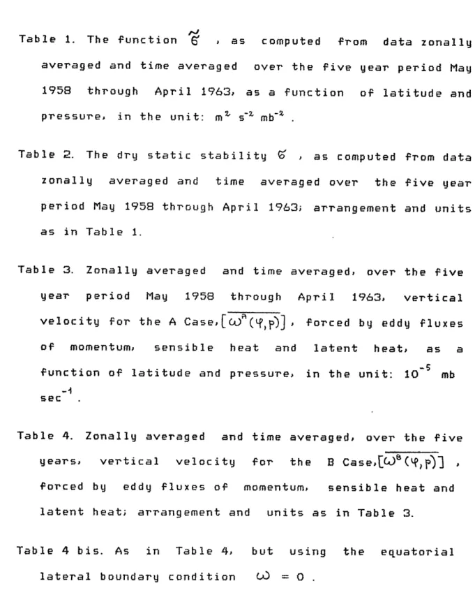
as computed from data zonally averaged and time averaged _{over the five year period May}

1958 through _{April 1963, as a function of latitude and} pressure, in the unit: m s S-71 mb- .

Table 2. The dry static stability 5 , as computed from data zonally averaged and time averaged over the five year period May 1958 through April 1963; arrangement and units as in Table 1.

Table 3. Zonally averaged _{and time averaged, over the five} year period May 1958 through April 1963, vertical

velocity for the A Case,[C"(qp)] forced by eddy fluxes

of momentum, sensible heat and latent heat, as a function of latitude and pressure, in the unit: 10 mb

sec

Table 4. Zonally averaged _{and time averaged, over the five}

years,

vertical

velocity

for

the

B

Case,[CIa('.?)1

forced by eddy fluxes of momentum, sensible heat and latent heat; arrangement and units as in Table 3.

Table 4 bis. As in Table 4, but using the equatorial lateral boundary condition &.) 0 .

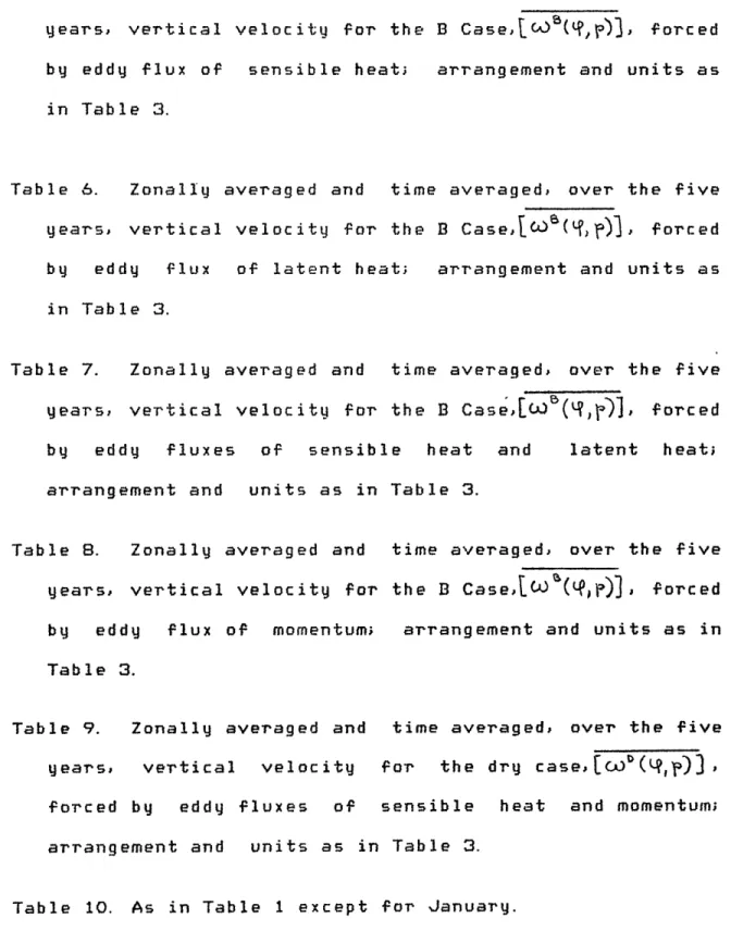
Table 5. Zonally averaged and time averaged, over the five

years, vertical velocity for the B Case,[i)(Q, &)3, forced by eddy flux of sensible heat; arrangement and units as

in Table 3.

Table 6. Zonally averaged and time averaged, over the five years, vertical velocity for the B Casej Cs(Lr], forced

by eddy flux of latent heat; arrangement and units as in Table 3.

Table 7. Zonally averaged and time averaged, over the five

years, vertical velocity for the B

Case,w0m(,V)),

forced

by eddy fluxes of sensible heat and latent heat; arrangement and units as in Table 3.

Table B. Zonally averaged and time averaged, over the five

years, vertical velocity for the B Case,I') (q9dP)I, forced

by eddy flux of momentum; arrangement and units as in Table 3.

Table 9. Zonally averaged and time averaged, over the five years, vertical velocity for the dry case,[C0'(9,p)], forced by eddy fluxes of sensible heat and momentum; arrangement and units as in Table 3.

Table 11.

Table 12.

As in Table 2 except for January.

As in Table 4 except for January.

Table 13. As in Table

Table 14. As in Table

Table 15. As in Table

Table 16. As in Table

5 except for January.

6 except 7 except 8 except for January. for January. for January.

Table 17. As in Table 1 except

Table 18. As in Table 2 except

Table 19. As in Table 4 except

Table 20. As in Table 5 except

Table 21. Table 22. Table 23. As in Table 6 except As in Table 7 except for July. for July. for July. for July. for July. for July.

W 4001 0.024 0.025 0.026 0.027 0.029 0.030 0.029 0.028 0.029 0.031 0.033 0.036 0.039 0.042 0.045 0.048 I 4 5001 0.014 0.014 0.016 0.017 0.018 0.018 0.017 0.016 0.017 0.018 0.019 0.021 0.022 0.022 0.024 0.025 I t 7001 -0.005 -0.005 -0.005 -0.003 -0.001 0.003 0.006 0.007 0.009 0.016 0.012 0.013 0.014 0.015 0.017 0.018 I 8501 _{-0.017 -0.017 -0.017 -0.016 -0.011 -0.006 -0.003 -0.000 0.002 0.006 0.010 0.010 0.011 0.015 0.019 0.021 I} 9001 -0.025 -0.024 -0.022 -0.020 -0.016 -0.013 -0.008 -0.004 -0.000 0.004 0.007 0.009 0.012 0.016 0.019 0.023 9501 -0.026 -0.025 -0.023 -0.022 -0.018 -0.015 -0.011 -0.006 0.001 0.005 0.006 0.009 0.012 0.016 0.019 0.024 1 --- --- --- ---0 5 10 15 20 25 30 35 40 45 50 55 60 65 70 75 LATITUDE Table 1 --- --- --- ---I _I 1001 2.164 2.140 2.131 2.130 2.101 2.101 2.101 2.103 2.100 2.094 2.107 2.116 2.128 2.138 2.148 2.157 1 2001 0.148 0.158 0.168 0.176 0.195 0.223 0.265 0.317 0.369 0.412 0.443 0.464 0.480 0.489 0.495 0.500 I 3001 0.045 0.046 0.047 0.050 0.054 0.060 0.068 0.077 0.089 0.102 0.116 0.128 0.139 0.147 0.155 0.164 I 4001 0.041 0.042 0.041 0.041 0.041 0.041 0.038 0.036 0.035 0.037 0.038 0.041 0.042 0.045 0.048 0.050 5001 0.035 0.035 0.033 0.032 0.032 0.031 0.029 0.027 0.026 0.026 0.026 0.026 0.027 0.027 0.027 0.028 7001 0.022 0.021 0.021 0.021 0.021 0.022 0.021 0.021 0.021 0.020 0.020 0.020 0.020 0.021 0.022 0.022 8501 0.016 0.016 0.015 0.016 0.016 0.017 0.019 0.018 0.017 0.017 0.017 0.017 0.018 0.020 0.023 0.025 | 9001 0.011 0.013 0.014 0.014 0.015 0.015 0.016 0.016 0.016 0.016 0.016 0.016 0.017 0.020 0.023 0.025 I 9501 0.0Q7 0.009 0.011 0.012 0.012 0.012 0.012 0.012 0.014 0.015 0.015 0.014 0.016 0.019 0.022 0.025 I --- --- --- --- ---0 5 10 15 20 25 30 35 40 45 50 55 60 65 70 75 LATITUDE Table 2

1 1 501 0.0 0.0 0.0 0.0 0.0 0.0 0.0 0.0 0.0 0.0 0.0 0.0 0.0 0.0 0.0 0.0 1001 0.3 0.3 0.3 0.0 -0.1 0.0 0.1 0.1 0.2 0.3 0.2 -0.0 -0.2 -0.5 -0.6 -0.6 | 2001 -4.2 -4.5 -4.1 -3.1 -0.6 1.6 2.1 1.0 0.4 0.6 -0.1 -0.7 -1.0 -1.3 -1.2 -0.7 1 3001 -12.0 -11.7 -9.3 -6.5 -2.4 2.1 4.7 3.4 1.5 1.0 -0.7 -1.7 -2.2 -2.2 -1.5 -0.2 I 4001 -11.4 -10.8 -10.0 -8.7 -4.0 2.1 5.6 4.6 3.0 2.1 -1.1 -2.8 -3.5 -2.9 -1.5 0.7 | 5001 -8.8 -8.3 -9.5 -10.4 -4.3 2.8 5.8 4.3 3.5 3.0 -1.0 -3.2 -4.3 -3.4 -1.4 1.3 I

8

7001 -0.4 2.5 -8.6 -9.6 -2.2 3.8 4.3 2.9 2.3 2.5 -0.2 -2.4 -3.9 -3.2 -0.9 1.1 8501 -2.4 2.7 -3.9 -5.5 -1.4 2.8 2.4 1.5 1.1 1.3 -0.1 -1.1 -2.4 -1.9 -0.4 0.3 I 9001 -10.5 0.9 -2.1 -3.6 -1.1 1.9 1.8 1.0 0.7 0.8 -0.0 -0.8 -1.7 -1.2 -0.3 0.2 9501 -13.8 -0.9 -0.7 -1.6 -0.6 0.9 1.0 0.6 0.3 0.4 0.0 -0.4 -0.8 -0.6 -0.2 0.1 10001 0.0 0.0 0.0 0.0 0.0 0.0 0.0 0.0 0.0 0.0 0.0 0.0 0.0 0.0 0.0 0.0 . --- --- ---0 5 10 15 20 25 30 35 40 45 50 55 60 65 70 75 LATITUDE Table 3 --- --- ---501 0.0 0.0 0.0 0.0 0.0 0.0 0.0 0.0 0.0 0.0 0.0 0.0 0.0 0.0 - 0.0 0.0 1001 0.3 0.4 0.3 0.1 -0.0 0.1 0.1 0.1 0.2 0.3 0.2 -0.1 -0.2 -0.5 -0.6 -0.6 2001 -3.6 -3.9 -3.5 -2.6 -0.3 1.7 2.0 0.9 0.4 0.5 -0.1 -0.7 -1.0 -1.3 -1.2 -0.7 3001 -10.4 -10.2 -7.9 -5.3 -1.7 2.1 4.5 3.1 1.4 1.0 -0.7 -1.7 -2.2 -2.2 -1.5 -0.2 I 4001 -8.7 -8.2 -7.4 -6.5 -3.0 2.0 5.1 4.1 2.8 2.1 -1.1 -2.8 -3.5 -2.9 -1.5 0.7 5001 -5.4 -4.7 -5.6 -6.6 -2.9 2.4 5.0 '3.6 3.3 3.0 -1.0 -3.2 -4.3 -3.4 -1.4 1.3 : 7001 0.0 0.0 0.0 0.0 0.0 2.1 2.6 1.8 2.2 2.4 -0.2 -2.4 -3.9 -3.2 -0.9 1.1 8501 0.0 0.0 0.0 0.0 0.0 0.0 0.0 0.0 1.0 1.2 -0.1 -1.1 -2.4 -1.9 -0.4 0.3 I 9001 0.0 0.0 0.0 0.0 0.0 0.0 0.0 0.0 0.7 0.8 -0.0 -0.8 -1.7 -1.2 -0.3 0.2 9501 0.0 0.0 0.0 0.0 0.0 0.0 0.0 0.0 0.3 0.4 0.0 -0.4 -0.8 -0.6 -0.2 0.1 I 10001 0.0 0.0 0.0 0.0 0.0 0.0 0.0 0.0 0.0 0.0 0.0 0.0 0.0 0.0 0.0 0.0 I I o --- --- ---- w---ft---ft---0 5 10 15 20 25 30 35 40 45 50 55 60 65 70 75 LATITUDE Table 4

400| 0 0 -2.2 -4.0 -4.7 -2.2 2.4 5.3 4.2 2. 9 2. 1 -1. 1 -2. 8 -3'.5 --2.9 -1. 5 0.7 5001 0.0 -0.6 -3.2 -5.3 -2.2 2.7 5.1 3.7 3.3 3.0 -1.0 -3.2 -4.3 -3.4 -1.4 1.3 -7031 0.0 0.0 0.0 0.0 0.0 2.2 2.6 1.8 2.2 2.5 -0.2 -2.4 -3.9 -3.2 -0.9 1.1 8501 0.0 0.0 0.0 0.0 0.0 0.0 0.0 0.0 1.0 1.3 -0.1 -1.1 -2.4 -1.9 -0.4 0.3 9001 0.0 0.0 0.0 0.0 0.0 0.0 0.0 0.0 0.7 0.8 -0.0 -0.8 -1.7 -1.2 -0.3 0.2 9501 0.0 0.0 0.0 0.0 0.0 0.0 0.0 0.0 0.3 0.4 0.0 -0.4 -0.8 - -0.6 -0.2 0.1 a 10001 0.0 0.0 0.0 0.0 0.0 0.0 0.0 0.0 0.0 0.0 0.0 0.0 0.0 0.0 0.0 0.0 - - - ---0 5 10 15 20 25 30 35 40 45 50 55 60 65 70 75 LATITUDE Table 4 bis old

000 000 0*0 000 0*0 000 000 000 000 000 0*0 000 000 0*0 0*0 000 b000t

To- TOO- 1O0- 000- -00- 0*0 0*0m Vo0 0*0 000 000 0*0 000 000 000 000 10G6

T *0- T*0- I*0- I*0- 0*0- 00- 0*0- 2*0- 000 0*0 000 000 000 000 0*0 000 1006 v

I

e-0OO0

3-0-

1*0 - *0-- 0-a 0o- *0- 0-0 00. 0-0 000 0-0 0-0 0*0 a*0 I099

I *0- ?-0- ?*0- Z-0- Z-0- 1-0- 1-0 9a0- b-0- 00 b-1 000 000 00 0*0 000 100±r

I £0- ZOO- ZO0- aa0 - Z0- 2'0- ZOO I*0- '0- 6'0, 01 * T O0- Sa0- 0 * 0110a T I os

I *0- *oo- ZO0- To- TOO- £0- T0O ZO- ZOO- 9*0 900 t0 boo- 200 q*T O loot,

I *0- 1-0- 1-0- 1-0- 1-0- ?*0- T*0 1-0- t-0- *0 a-0 to To- b-0 00 1*0- oos

| *0- T*0- t*0 - *0- T*0 -0- 0*0- 0*0- 0*0- T*0 ₁₀ T*0 *0 *0 *0 T*0 100 S 0*0- 0*0- 0*0- 0*0- 0*0- 000- 0*0- 0*0- 0*0 000 000 000 0*0 000 000 0*0 1001 I 000 000 0*0 000 000 000 0*0 000 0*0 000 000 0*0 000 000 0*0 000 |09 0* OL G9 09 * 0*0 0* 00 0* 0* 0* 00 *1 01 9 0 I I 1 0~000 0 0 000 0 00 000 0 0 0 0 00 000 000 000 0 0 000 00 60 000 000 1 0001 I T0- *0- T*0- Z*0- a*0- T*0 T*0 T*0 000 000 0*0 0*0 000 000 0*0 000 1096 l *- *0-0- 9*0- 0- *0- *0 900 Z*0 000 000 000 000 000 0*0 000 000 1006

20-0- go0- go0- Le- go0- T-0 L-0 b-0 000 0-0 000 000 000 0*0 000 0-fn 10Gg

bI

~0-

? I- 4?aT - !£*T - 01 a P Ia0 e aT L a0 Bo0 bo1 900 00a0 000 000 00a0 00a0 Io 00 tn

1 oo b~O f*T- 9a T- 9 a1- 0 &T- I1 0T L a0 0 aT1 0 a Lai a*T- a*2- T*- 6*?- Go?- loos

I-T 6~0 ao1 01 $,- 00a0 0O T * T00 a T L 0 L1 a 2aT - 2*- 0 a b- 64v- G9 I0 ,

I *O TO0TP- 001T- TOT- L0O- 000 900 bo PTT 20? 901 6*0- T*2- Lob- V9- 9*b- 1o0s

Goo0- goo- TOT- 001- goo- 1o0 000 Le0 TO OO1 0t O 900 - T 1- G*C- 2*- loo?

2*0-

00- 00- b*0- Z*0-

1*0

2*0

E0

3*0

?* 0 *o Z*0- T*o- 00- 0*0 000- 001

000 0*0 000 0*0 0*0 0*0 0*0 0*0 000 000 000 000 000 000 0*0 00

109