Atmospheric carbonyl sulfide (OCS) variation from 1992?2004 by ground-based solar FTIR spectrometry

(1)

HAL Id: hal-00301051

https://hal.archives-ouvertes.fr/hal-00301051

Submitted on 2 Mar 2006

HAL is a multi-disciplinary open access

archive for the deposit and dissemination of sci-entific research documents, whether they are pub-lished or not. The documents may come from teaching and research institutions in France or abroad, or from public or private research centers.

L’archive ouverte pluridisciplinaire HAL, est destinée au dépôt et à la diffusion de documents scientifiques de niveau recherche, publiés ou non, émanant des établissements d’enseignement et de recherche français ou étrangers, des laboratoires publics ou privés.

Atmospheric carbonyl sulfide (OCS) variation from

1992?2004 by ground-based solar FTIR spectrometry

N. M. Deutscher, N. B. Jones, D. W. T. Griﬀith, S. W. Wood, F. J. Murcray

To cite this version:

N. M. Deutscher, N. B. Jones, D. W. T. Griﬀith, S. W. Wood, F. J. Murcray. Atmospheric carbonyl sulfide (OCS) variation from 1992?2004 by ground-based solar FTIR spectrometry. Atmospheric Chemistry and Physics Discussions, European Geosciences Union, 2006, 6 (2), pp.1619-1636. �hal-00301051�

(2)

ACPD

6, 1619–1636, 2006 OCS variations by FTIR spectrometry N. M. Deutscher et al. Title Page Abstract Introduction Conclusions References Tables Figures J I J I Back Close Full Screen / Esc

Printer-friendly Version Interactive Discussion

EGU Atmos. Chem. Phys. Discuss., 6, 1619–1636, 2006

www.atmos-chem-phys-discuss.net/6/1619/2006/ © Author(s) 2006. This work is licensed

under a Creative Commons License.

Atmospheric Chemistry and Physics Discussions

Atmospheric carbonyl sulfide (OCS)

variation from 1992–2004 by

ground-based solar FTIR spectrometry

N. M. Deutscher1, N. B. Jones1, D. W. T. Griffith1, S. W. Wood2, and F. J. Murcray3

1

Department of Chemistry, University of Wollongong, Wollongong, NSW, Australia

2

National Institute of Water and Atmospheric Research, Lauder, Central Otago, New Zealand

3

Department of Physics, University of Denver, Denver, Colorado, USA

Received: 8 November 2005 – Accepted: 22 December 2005 – Published: 2 March 2006 Correspondence to: N. M. Deutscher ([email protected])

(3)

ACPD

EGU

Abstract

Analysis of ground-based high-resolution solar FTIR absorption spectra from four sites was performed to determine trends and variability in OCS columns over the period 1992–2004. The sites were Wollongong, Australia (34.45◦S, 150.88◦E), Lauder, New Zealand (45.0◦S, 169.7◦E), Arrival Heights, Antarctica (77.8◦S, 166.6◦E) and Mauna

5

Loa, Hawaii (19.5◦N, 155.6◦W). Small but significant long-term trends of −0.18±0.02% yr−1 above Hawaii, −0.30±0.12% yr−1 above Wollongong and −0.29±0.14% yr−1 above Lauder, were seen. No significant trend was seen above Arrival Heights. A large peak-to-peak seasonal difference observed in 1996–1997 above Wollongong and re-ported earlier was confirmed, but not repeated in later years. This seasonal feature

10

correlated with particularly high water vapour columns present during late summer and early autumn, and suggests a link to warm oceanic airmasses. Seasonal variation of approximately 6% per year is observed in the total column in other years for all four locations.

1 Introduction

15

Since the discovery of the stratospheric sulfate aerosol (SSA) layer (Junge et al., 1961), great interest has been focussed on determining the source of sulfur that maintains the aerosol levels. The SSA layer is important because of its effect on the radiative balance of the earth and consequent influence on climate (Turco et al., 1980), and its influence on ozone distribution (Ko et al., 2003; Pitari and Mancini, 2002). Volcanic eruptions are

20

known to provide a large amount of sulfur, in the form of sulfur dioxide (SO₂), directly to the stratosphere (Crutzen, 1976; Ko et al., 2003). However the source of sulfur that maintains the aerosol levels between large eruptions is uncertain and is the subject of considerable debate (Kjellstrom, 1998; Leung et al., 2002; Pitari et al., 2002; Sturges et al., 2001).

25

(4)

sul-ACPD

EGU fur to the aerosol layer in quiescent periods, because of its relative abundance and

long lifetime compared to other sulfur trace gases. Indeed OCS has a lifetime of the order of years (Bandy et al., 1992; Brimblecombe, 1996; Sturges et al., 2001) com-pared to hours to days for other significant sulfur trace gases such as carbon disulfide (CS₂), hydrogen sulphide (H₂S), dimethyl sulfide (DMS – (CH₃)₂S) and sulfur dioxide

5

(SO₂) (Brimblecombe, 1996). This lifetime, combined with an abundance of the or-der of 500 pmol mol−1 (pptv), (compared to mole fractions in the range of 5–100 pmol mol−1 for the other sulfur trace gases), allows OCS to be transported to the lower stratosphere, where it can be either photolysed or oxidised to sulfate (Brimblecombe, 1996).

10

As a result of the potential for OCS to be a sulfate aerosol source, the global budget of OCS is of interest. Currently, the budget is balanced to within the levels of uncer-tainty (Kettle et al., 2002; Watts, 2000), however the uncertainties involved are large, particularly those surrounding the flux of OCS from the ocean to the atmosphere.

Previous work from this laboratory (Griffith et al., 1998) showed a large seasonal

15

difference in total column amounts at Wollongong, Australia (34.45◦S, 150.88◦E, 30 m a.s.l.), with late summer peak and winter trough, from data collected between May 1996 and March 1997. This difference was tentatively attributed to a warm coastal ocean source. Analysis of further data from ensuing years is necessary to confirm this conjecture. Data from other locations with oceanic influence are also desirable for

com-20

parative purposes. The altitude at which the variation occurs is also of interest. This paper extends the original study of Griffith et al. (1998) to 4 sites, from 1992 to 2004.

The long-term OCS trend was reported as being insignificant before 1991 (Bandy et al., 1992). Recent trends of −0.8±0.5% yr−1 over 10 years (Sturges et al., 2001) and −0.25±0.04% yr−1 over 24 years (Rinsland et al., 2002) have been observed in the

25

northern hemisphere, with no observed southern hemispheric long-term trend based on observations (Sturges et al., 2001). However, an inverse approach based on a one-dimensional forward diffusion model using measurements of air from polar firn, ice cores and ambient atmosphere was used to calculate an inferred atmospheric history

(5)

ACPD

EGU that suggested a 10–16% decrease in 10–15 years from the 1980s (Montzka et al.,

2004). These long-term downward trends agree with recent reported decreases in OCS source strength in the northern hemisphere (Montzka et al., 2004; Sturges et al., 2001) and suggest that the effects of this are beginning to filter through to the southern hemisphere.

5

An interhemispheric ratio (IHR) can be calculated using the following formulation:

Mean northern hemisphere measurement/mean southern hemisphere measurement

In recent previous works these have been calculated to be 1.14±0.06 (Griffith et al.,

10

1998; Rinsland et al., 1992), 1.09±0.07 (Sturges et al., 2001) and 1.05 (Kjellstrom, 1998), indicative of a larger abundance of OCS in the northern hemisphere.

The dependence of OCS levels on altitude has also been examined. Very little change is observed with altitude throughout the troposphere (Chin and Davis, 1995), with volume mixing ratios decreasing rapidly above the tropopause until negligible

lev-15

els are reached above 25–30 km (Engel and Schmidt, 1994). This decrease occurs be-cause the major non-surface sinks for OCS, photolysis and oxidation (Chin and Davis, 1993, 1995; Kettle et al., 2002; Watts, 2000), occur mainly in the stratosphere.

The results presented in this paper examine long term trends and the variation of OCS with height in the atmosphere, and attempt to identify oceanic influence on OCS

20

columns. Three oceanic sites, one in the northern and two in the southern hemisphere, and an inland southern hemisphere site are used to determine the influence of the ocean.

2 Methods

Infrared absorption spectra of the atmosphere have been recorded, using solar remote

25

sensing coupled to high resolution FTIR spectrometers. For further details of solar FTIR spectroscopy and analysis of solar spectra see Griffith et al. (1998). Table 1

(6)

ACPD

EGU summarises the site locations, instrumentation and measurements.

All spectra were analysed using SFIT 2 (Pougatchev et al., 1995; Rinsland et al., 1998), which uses optimal estimation based on the formulism of Rodgers (2000) com-bined with a Newtonian iteration to account for the non-linear nature of atmospheric absorption. The optimal estimation inverse model in SFIT2 takes advantage of the

5

pressure broadening of spectral lines to determine altitude dependence, which for the case of OCS results in approximately 3 independent vertically resolved layers. Before fitting, the IR spectra were selected to have a zero level offset of less than 5% and a signal-to-noise ratio (SNR) of greater than 100, where the SNR is defined as:

10

SNR= Signal level in spectrum/Random noise level in spectrum

Spectra with an rms residual of the fit of less than 0.4% were included in the post-fitting analysis.

The assumed apriori OCS vertical profile for each site was based on Griffith et

15

al. (1998), and adjusted between sites to account for expected variation in tropopause heights. Absorption coefficients in the forward model were calculated using line param-eters from the Hitran 2000 database (Rothman et al., 2001). For all four locations, daily temperature and pressure profiles were used, each with temperature and pressure de-fined at 18 different heights specific to the individual site. This data was obtained from

20

the American National Meteorological Centre (NMC) and uses a combination of data obtained from satellites and local sondes. Other parameters in the forward model in-clude instrumental lineshape, a solar reference spectrum, wavelength shift and zero offset.

The spectral microwindows chosen for the analysis are based upon the OCS ν₃

25

band centred around 2060 cm−1. The microwindows selected were the 2045.00– 2045.85 cm−1(2045 cm−1) region surrounding the 2045.578488 cm−1P37 line, and the 2055.20–2057.70 cm−1 (2056 cm−1) region containing the 2055.860551 cm−1 (P15), 2056.300189 cm−1 (P14) and 2056.737410 cm−1 (P13) lines of the OCS ν₃ band.

(7)

ACPD

EGU These microwindows were used consistently on spectra taken from each of the four

sites, with the two microwindows fitted simultaneously on each spectrum. Water vapour (H₂O), carbon dioxide (CO₂), carbon monoxide (CO) and ozone (O₃) were also actively fitted and co-retrieved. SFIT 2 was used to resolve the total columns retrieved into three altitude regions – 0–4 km, 4–12 km and 12–100 km above mean sea level. This roughly

5

corresponds to two layers in the troposphere and a single stratospheric layer. Using the formulism of Rodgers (1998) both the averaging kernels, and degrees of freedom for signal (d.o.f.s) were calculated to help determine the appropriate layer boundaries for the selection of partial columns. The degrees of freedom for signal determined for the total column was 2.7 for fitting the 2045 cm−1 and 2056 cm−1 windows

simultane-10

ously using a simulated spectrum at solar zenith angle 61.68◦. This corresponds to 0.6, 0.9 and 1.2◦ of freedom for the 0–4 km, 4–12 km and 12–100 km partial columns, respectively. The independence of the vertical layers was determined for a suite of spectra both visually from plots of averaging kernels and numerically from the reported degrees of freedom for signal.

15

3 Results and discussion

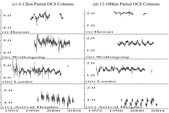
Figure 1 presents the monthly mean retrieved total and partial OCS columns for each site over the period of analysis. The mean pressure corrected total columns, relative standard errors, trends and peak-to-peak amplitudes are summarised in Table 2. All total columns reported and discussed in this section are scaled to sea level for

20

comparison, using the simple conversion:

Pressure corrected total column= column above site * 1013/mean site pressure Above Wollongong, the seasonal variation is much larger in 1996–1997 (27%) than

25

for any other period at any site. The intra-year variation at Wollongong over the pe-riod of the rest of the study was of the order of 11% peak-to-peak. However, this

(8)

ACPD

EGU seasonal behaviour was not simply sinusoidal, nor does it follow any constant pattern

within the period of each year. The anomalous variation in 1996–1997 confirms the large value noted by Griffith et al. (1998) (18%) but it is not repeated in later years. The higher apparent amplitude in the present study is most likely due to the different analysis algorithms used: Griffith et al. (1998) used a simple profile scaling approach

5

in which altitude profiles of pressure and temperature were fixed and trace gas con-centration profiles were fixed in shape but scaled in magnitude to attain best fit to the measured spectra. This approach smooths over some seasonal variability, in particu-lar in tropopause height and temperature. The profile retrieval approach used in the present study allows for daily pressure-temperature profile variation and fits the shape

10

as well as the magnitude of the OCS vertical profile.

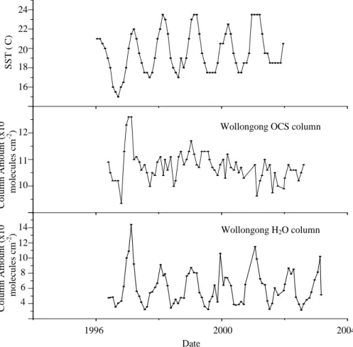
Figure 2 shows the monthly mean total OCS column amounts, monthly mean total column H₂O amounts and monthly mean sea surface temperature (SST) for the coastal ocean off Wollongong. The SSTs are adapted from data available online (National Oceanographic Data Center, 2003), where they are displayed in the form of isotherm

15

plots with a resolution of one degree celsius. A numerical value was given by observing the pixel corresponding to the ocean to the east of Wollongong, and assigning the value from the isotherm at that point. The SSTs are available for the period up until December 2001.

From Fig. 2, it can be seen that of the years with available SST data that coincide

20

with the period of spectral collection in Wollongong, the 1996–1997 period has the lowest temperature. In the following years, apart from 1999–2000, the peak summer SST is at least one degree Celsius warmer, as are the minimum SSTs in the winters following 1996.

Griffith et al. (1998) hypothesised that the large seasonal variation in column OCS

25

was due to a local coastal ocean source, driven by seasonal changes in ocean surface temperature coupled with easterly onshore winds in summer. Clearly this large sea-sonal variation does not correlate with SST variations and is not present in subsequent years, and therefore strongly suggests that ocean temperature is not the main driver of

(9)

ACPD

EGU OCS column changes off the coast of Wollongong. However, retrieval of H₂O columns

from the same spectra shows anomalously high water vapour total columns highly cor-related with the high OCS columns (Fig. 2). Meteorological conditions could have led to maritime airmasses in 1996–1997, resulting in the high OCS and water seen at the time. In summary, high OCS does appear to be correlated to the presence of moist

5

airmass, but this is not driven by higher SST.

Comparing column amounts from Wollongong and Lauder, two important points can be noted. Firstly, the mean values for the two sites are consistent, as expected for sites that are both situated in the southern hemisphere and mid-latitude. Secondly, the variation within the course of each year is less at Lauder than at Wollongong.

10

Compared to Wollongong, Lauder is situated inland, removing it from potential oceanic influence. The reduced variation seen at Lauder could result from the damping of signals caused by oceanic fluxes.

Figures 1(iv) show the total and partial columns above Arrival Heights, Antarctica. The gaps in this dataset between April and August each year are due to the absence

15

of sunlight necessary for collection of solar infrared spectra. The mean total column above the Antarctic site is 9.4±0.2×1015molecules cm−2. This OCS total column is relatively low compared to the other three sites, being 8% lower than the two southern hemisphere mid-latitude sites. This is caused in part by the relatively low tropopause height, and hence lower altitude at which OCS mixing ratios begin to decrease. The

20

low total column may also be due to the relatively long distance from sources, such as northern hemisphere industrial sources and the open ocean. The distance of the site from the open ocean due to surrounding sea ice varies from around 20 km or less in summer to several hundred kilometres in winter. However the long atmospheric lifetime for OCS in comparison to the timescale for atmospheric transport suggests that this

25

effect would be small when compared with other southern hemisphere locations. The OCS total column above Arrival Heights shows seasonal variation with amplitude of 7– 8%. Comparing concurrent measurements from this work and surface concentration measurements at the South Pole from Montzka et al. (2004), reveals similar phase and

(10)

ACPD

EGU magnitude in seasonality.

Figures 1(i) show the total and partial columns above Hawaii. The OCS total column amounts above Hawaii appear to show some seasonal dependence. The gap in the data between April 1999 and April 2001 was due to instrumental problems. The 0–4 km partial column is very low because of the site altitude, 3460 m.

5

The seasonal OCS cycle observed in the troposphere above Hawaii correlates with surface temperatures in the surrounding ocean (National Oceanographic Data Center, 2003). The persistence of the cycle above Hawaii compared to that above Wollongong is probably caused by the island nature of the Hawaiian site. That is, there is a con-sistent oceanic influence regardless of the direction from which the sampled airmass

10

originated.

Spectra were collected at Mauna Loa predominantly at two specific times of the day, around 8.00 a.m. and 5.00 p.m. local time. Separating the measurements into morn-ing and afternoon clusters, the mornmorn-ing tropospheric OCS columns are 2.8% higher than the afternoon columns. The difference is significant at the 95% probablility level.

15

This morning-afternoon difference is related to a previously reported phenomenon on Mauna Kea (Ferguson, 1991), where morning downslope winds move air from the Mauna Loa caldera into the observed airpath, resulting in increased sulphur concen-trations.

3.1 Trends

20

Fitting least-squares linear regressions to the total OCS columns above Wollon-gong and Lauder gave long-term downward trends of −0.30±0.12% OCS/year and −0.29±0.14% OCS/year, respectively, over the period of the dataset. These trends are small, but statistically significant, and consistent within the range of errors. Since both locations are mid-latitude southern hemisphere sites (and only 14◦ of longitude

25

apart), the agreement between these trends is not surprising. No significant trend was observed in the total OCS column above Arrival Heights. The fact that both Wollon-gong and Lauder have downward trends is of particular interest. Previous work has

(11)

ACPD

EGU seen no significant long-term southern hemispheric trend, whereas an overall northern

hemispheric decrease in OCS has been observed (Sturges et al., 2001). The north-ern hemispheric trend is attributed to decreasing emissions from industrial sources, while there are few southern hemispheric industrial sources. The decreased industrial emissions signature observed in the northern hemisphere should carry through to the

5

southern hemisphere in approximately 1–2 years. The source terms in the southern hemisphere are dominated by oceans and biomass burning, which are highly variable and are not likely to be as well defined or measurable as the decreasing industrial emissions observed in the northern hemisphere.

There is a global latitudinal trend, with the OCS column amounts decreasing from

10

north to south with increased distance from the majority of industrial sources. The IHR is calculated over the length of the study from the ratio of the mean northern and southern hemispheric pressure adjusted total columns. This value is 1.12±0.07, in agreement with other values in recent literature (Griffith et al., 1998; Kjellstrom, 1998; Sturges et al., 2001).

15

The small downward trend of −0.18±0.02% OCS/year observed at Hawaii con-firms the decreasing industrial OCS emissions. This trend is much smaller than the 0.8±0.5% OCS/year recently observed (Sturges et al., 2001).

4 Conclusions

This study confirms that the large seasonal variation observed previously in 1996–

20

1997 in Wollongong was real, but finds that it is not repeated in following years. The reanalysis finds that the cycle had peak-to-peak amplitude of 27% (c.f. 18%) and a late summer maximum. The difference in cycle amplitudes is attributed to the different anal-ysis algorithms, in particular the treatments of tropopause heights and a priori profiles between the two techniques. An anomalously high level of water vapour accompanied

25

the high level of OCS observed during that period. The relationship between water vapour and OCS suggests that they both have a common ocean source. The seasonal

(12)

ACPD

EGU cycle observed occurred largely in the 0–4 km and 4–12 km partial columns. Small

sea-sonal variation was observed in the data at all sites and in other years (Wollongong, Lauder, Arrival Heights, and Hawaii) with peak-to-peak amplitudes of approximately 6%. These variations did not fit a sinusoidal cycle well, showing the natural variability of OCS over the period of a year.

5

The long-term OCS trends were also analysed at all sites. The columns at Lauder and Wollongong were found to be decreasing by small, but statistically significant amounts of −0.29±0.14% yr−1and −0.30±0.12% yr−1, respectively. These trends are consistent within the standard errors, and indicative of a reduced level of anthropogenic OCS emissions. The total column trend above Hawaii was also found to be decreasing

10

at a rate of −0.18±0.02% yr−1, while the trend above Arrival Heights (−0.10±0.10 % yr−1) was not significantly different from zero.

The data were also used to calculate an interhemispheric ratio of 1.12±0.07, con-sistent with previous recent results. The northern hemisphere abundances are higher than those in the southern hemisphere due to larger anthropogenic emissions.

15

Acknowledgements. The authors acknowledge the University of Wollongong, NIWA and the

University of Denver for financial support, and especially support given by the Australian Re-search Council, New Zealand Foundation for ReRe-search Science and Technology, and Antarctica New Zealand.

References

20

Bandy, A. R., Thornton, D. C., Scott, D. L., Lalevic, M., Lewin, E. E., and Driedger III, A. R.: A time series for carbonyl sulfide in the northern hemisphere, J. Atmos. Chem., 14, 527–534, 1992.

Brimblecombe, P.: Air composition & chemistry, Cambridge University Press, Cambridge, 1996.

25

Chin, M. and Davis, D. D.: Global sources and sinks of ocs and cs₂ and their distributions, Global Biogeochem. Cycles, 7, 321–337, 1993.

(13)

ACPD

EGU

Chin, M. and Davis, D. D.: A reanalysis of carbonyl sulfide as a source of stratospheric back-ground sulfur aerosol, J. Geophys. Res., 100, 8993–9005, 1995.

Crutzen, P. J.: The possible importance of cso for the sulfate layer of the stratosphere, Geophys. Res. Lett., 3, 73–76, 1976.

Engel, A. and Schmidt, U.: Vertical profile measurements of carbonylsulfide in the stratosphere,

5

Geophys. Res. Lett., 21, 2219–2222, 1994.

Griffith, D. W. T., Jones, N. B., and Matthews, W. A.: Interhemispheric ratio and annual cycle of carbonyl sulfide (ocs) total column from ground-based solar ftir spectra, J. Geophys. Res., 103, 8447–8454, 1998.

Junge, C. E., Chagnon, C. W., and Manson, J. E.: Stratospheric aerosols, J. Meteorol., 18,

10

81–108, 1961.

Kettle, A. J., Kuhn, U., von Hobe, M., Kesselmeier, J., and Andreae, M. O.: Global budget of atmospheric carbonyl sulfide: Temporal and spatial variations of the dominant sources and sinks, J. Geophys. Res., 107, 4658–4673, 2002.

Kjellstrom, E.: A three-dimensional global model study of carbonyl sulfide in the troposphere

15

and the lower stratosphere, J. Atmos. Chem., 29, 151–177, 1998.

Leung, F.-Y. T., Colussi, A. J., Hoffmann, M. R., and Toon, G. C.: Isotopic fractionation of carbonyl sulfide in the atmosphere: Implications for the source of background stratospheric sulfate aerosol, Geophys. Res. Lett., 29, doi:10.1029/2001GL013955, 2002.

Montzka, S. A., Aydin, M., Battle, M., Butler, J. H., Saltzman, E. S., Hall, B. D., Clarke,

20

A. D., Mondeel, D., and Elkins, J. W.: A 350 year atmospheric history for carbonyl sulfide inferred from antarctic firn air and air trapped in ice, J. Geophys. Res., 109, doi:10.1029/2004JD004686, 2004.

National Oceanographic Data Center: Monthly-averaged sst fields,http://www.nodc.noaa.gov/

dsdt/oisst/oisstmon.htm, 2003.

25

Pitari, G. and Mancini, E.: Short-term climatic impact of the 1991 volcanic eruption of mt. Pinatubo and effects on atmospheric tracers, Nat. Hazards Earth Syst. Sci., 2, 91–108, 2002.

Pitari, G., Mancini, E., Rizi, V., and Shindell, D. T.: Impact of future climate and emission changes on stratospheric aerosols and ozone, J. Atmos. Sci., 59, 414–440, 2002.

30

Pougatchev, N. S., Connor, B. J., and Rinsland, C. P.: Infrared measurements of the ozone vertical distribution above kitt peak, J. Geophys. Res., 100, 16 689–16 697, 1995.

(14)

ACPD

EGU

T., Stephen, T. M., and Chiou, L. S.: Ground-based infrared spectroscopic measurements of carbonyl sulfide: Free tropospheric trends from a 24-year time series of solar absorption measurements, J. Geophys. Res., 107, 4657–4665, 2002.

Rinsland, C. P., Jones, N. B., Connor, B. J., Logan, J. A., Pougatchev, N. S., Goldman, A., Murcray, F. J., Stephen, T. M., Pine, A. S., Zander, R., Mahieu, E., and Demoulin, P.:

North-5

ern and southern hemisphere ground-based infrared spectroscopic measurements of tropo-spheric carbon monoxide and ethane, J. Geophys. Res., 103, 28 197–28 217, 1998.

Rinsland, C. P., Zander, R., Mahieu, E., Demoulin, P., Goldman, A., Ehhalt, D. H., and Rudolph, J.: Ground based infrared measurements of carbonyl sulfide total column abundances: Long-term trends and variability, J. Geophys. Res., 97, 5995–6002, 1992.

10

Rodgers, C. D.: Information content and optimisation of high spectral resolution remote mea-surements, Remote Sensing: Inversion Problems and Natural Hazards, Adv. Space Res., 21, 361–367, 1998.

Rodgers, C. D.: Inverse methods for atmospheric sounding – theory and practice, World Sci-entific, London, 2000.

15

Rothman, L. S., Barbe, A., Chris Benner, D., Brown, L. R., Camy-Peyret, C., Carleer, M. R., Chance, K., Clerbaux, C., Dana, V., and Devi, V. M.: The hitran molecular spectroscopic database: Edition of 2000 including updates through 2001, J. Q. S. Rad. Trans., 82, 5–44, 2001.

Sturges, W. T., Penkett, S. A., Barnola, J.-M., Chappellaz, J., Atlas, E., and Stroud, V.: A

20

long-term record of carbonyl sulfide (cos) in two hemispheres from firn air measurements, Geophys. Res. Lett., 28, 4095–4098, 2001.

Turco, R. P., Whitten, R. C., Toon, O. B., Pollack, J. B., and Hamill, P.: Ocs, stratospheric aerosols and climate, Nature, 283, 283–286, 1980.

Watts, S. F.: The mass budgets of carbonyl sulfide, dimethyl sulfide, carbon disulfide and

hy-25

(15)

ACPD

EGU

Table 1. Site locations, instruments and period of measurement.

Site Lat Long Alt Instrument Period No. of (m a.s.l.) measurements Arrival Heights, Antarctica 77.8◦S 166.6◦E 200 Bruker 120-M 1997–2003 496

Lauder, New Zealand 45.0◦S 169.7◦E 370 Bruker 120-HR April–Sep 1992, 3029 and 2002–2003 Bruker 120-M Sep 1992–2001 Mauna Loa, Hawaii 19.5◦N 155.6◦W 3460 Bruker 120-HR 1995–2001 767 Wollongong, Australia 34.5◦S 150.9◦E 30 Bomen DA8 1996–2003 2462

(16)

ACPD

EGU

Table 2. Mean pressure, pressure corrected total columns, relative standard errors in the mean

total columns, linear trends and yearly peak-to-peak amplitudes for all sites.

Site Mean pressure Mean column Relative std Trend Ampl. p-p (mb) (×1016molec cm−2) error (%) (%/yr) (%) Arrival Heights 989 0.94±0.02 2.4 −0.10±0.10 7.0 Hawaii 674 1.13±0.04 3.7 −0.18±0.02 6.4 Lauder 971 1.02±0.04 4.1 −0.29±0.14 8.0

Wollongong 1013 1.07±0.03 2.8 −0.30±0.12 27.0 (1996–1997) 11.4 (1997–2003)

(17)

ACPD

Printer-friendly Version Interactive Discussion EGU 1992 1996 2000 2004 2.0 4.0 6.0

(iv) Arrival Heights 2.0 4.0 6.0 (iii) Lauder 2.0 4.0 6.0 (ii) Wollongong 0.25 0.50 0.75 (i) Hawaii

(b) Below 4km Partial OCS Columns

1992 1996 2000 2004

8 10 12

(iv) Arrival Heights 8 10 12 (iii) Lauder 8 10 12 (ii) Wollongong 8 10 12 (i) Hawaii

(a) Pressure Corrected Total OCS Columns

Fig. 1. (a–b) Monthly mean pressure corrected total columns and below 4 km partial columns

for all 4 sites. In each section of the figure the sites are arranged by latitude from north to south (top to bottom), and the units are ×1015molecules cm−2. In each subplot (a–b) the vertical axes are the same, apart from (b(i)).

(18)

ACPD

Printer-friendly Version Interactive Discussion EGU 1992 1996 2000 2004 1.0 2.0

(iv) Arrival Heights 1.0 2.0 (i) Hawaii 1.0 2.0 (ii) Wollongong 1.0 2.0 (iii) Lauder

(d) 12-100km Partial OCS Columns

1992 1996 2000 2004

4.0 5.0

(iv) Arrival Heights 4.0 5.0 (iii) Lauder 4.0 5.0 (ii) Wollongong 4.0 5.0 (i) Hawaii

(c) 4-12km Partial OCS Columns

Fig. 1. (c–d) Monthly mean (c) 4–12 km partial columns and (d) 12–100 km partial columns for

all 4 sites. As in Fig. 1a–b sites are arranged by latitude from north to south (top to bottom), all units are ×1015molecules cm−2and all vertical axes are on the same scale.

(19)

ACPD

EGU

Date

1996 2000 2004

Wollongong Sea Surface Temp

Wollongong H2O column

Wollongong OCS column

S S T ( C ) 24 22 18 20 16 C ol um n A m ount ( x10 1 5 m ol ec ul es c m -2 ) 12 11 10 C ol um n A m ount ( x 10 2 2 m ol ec ul es c m -2 ) 14 12 10 8 6 4

Fig. 2. Wollongong sea surface temperatures (◦C, top panel), total OCS column amounts (×1015molecules cm−2, centre panel) and water columns (×1022molecules cm−2, bottom panel).