Modelling representation errors of atmospheric CO₂ concentrations at a regional scale

HAL Id: hal-00303977

https://hal.archives-ouvertes.fr/hal-00303977

HAL is a multi-disciplinary open access

archive for the deposit and dissemination of sci-entific research documents, whether they are pub-lished or not. The documents may come from teaching and research institutions in France or abroad, or from public or private research centers.

L’archive ouverte pluridisciplinaire HAL, est destinée au dépôt et à la diffusion de documents scientifiques de niveau recherche, publiés ou non, émanant des établissements d’enseignement et de recherche français ou étrangers, des laboratoires publics ou privés.

Modelling representation errors of atmospheric CO2

concentrations at a regional scale

L. F. Tolk, A. G. C. A. Meesters, A. J. Dolman, W. Peters

To cite this version:

L. F. Tolk, A. G. C. A. Meesters, A. J. Dolman, W. Peters. Modelling representation errors of atmospheric CO2 concentrations at a regional scale. Atmospheric Chemistry and Physics Discussions, European Geosciences Union, 2008, 8 (1), pp.3287-3312. �hal-00303977�

ACPD

Printer-friendly Version Interactive Discussion Atmos. Chem. Phys. Discuss., 8, 3287–3312, 2008

www.atmos-chem-phys-discuss.net/8/3287/2008/ © Author(s) 2008. This work is distributed under the Creative Commons Attribution 3.0 License.

Atmospheric Chemistry and Physics Discussions

Modelling representation errors of

atmospheric CO

₂

concentrations at a

regional scale

L. F. Tolk1, A. G. C. A. Meesters1, A. J. Dolman1, and W. Peters2

1

VU University Amsterdam, Amsterdam, The Netherlands

2

Wageningen University and Research Centre, Wageningen, The Netherlands

Received: 9 January 2008 – Accepted: 14 January 2008 – Published: 15 February 2008 Correspondence to: L. F. Tolk (lieselotte.tolk@falw.vu.nl)

ACPD

Printer-friendly Version Interactive Discussion

Abstract

Inverse modelling of carbon sources and sinks requires an accurate estimate of the quality of the observations to obtain a realistic estimate of the inferred fluxes and their uncertainties. Representation errors, defined here as the mismatch between point ob-servations and grid cell averages, may add substantial uncertainty to the interpretation

5

of atmospheric CO2 concentration data. We used a high resolution (2 km) mesoscale

model (RAMS) to simulate the variations in the CO₂ concentration to estimate the representation errors for grid sizes of 10–100 km. Meteorology is the main driver of representation errors in our study causing spatial and temporal variations in the error estimate. Within the nocturnal boundary layer the representation errors are relatively

10

large and mainly determined by unresolved topography at lower model resolutions. During the day, surface CO2 flux variability and mesoscale circulations were found to

be the main sources of representation errors. Careful up-scaling of point observations can reduce the importance of the representation error substantially. The remaining representation error is in the order of 0.5–1.5 ppm at 20–100 km resolution.

15

1 Introduction

Understanding the variation in atmospheric CO2concentration is key to prediction and

quantification of global climate change. Terrestrial CO2 fluxes have a major impact on

the global and regional CO₂ concentration levels and it is therefore important to un-derstand their spatial and temporal variation. Since the atmosphere is on the short

20

term an incomplete mixer of the CO2 surface fluxes, observations of CO2

concentra-tions can be used to quantify the magnitude and strength of the surface fluxes. At the global scale, such inversion studies have increased our knowledge about the terrestrial source-sink distribution, but exact estimates of the sources and sink still vary consid-erably (e.g. Fan et al 1998; Bousquet et al., 1999; Gurney et al., 2002; R ¨odenbeck et

25

ACPD

Printer-friendly Version Interactive Discussion are associated with errors in the simulated atmospheric transport (Gurney et al., 2002;

Yang et al., 2007; Stephens et al., 2007), aggregation of the surface fluxes over large areas (Kaminski et al., 2001), errors due to a poor representation of the diurnal and seasonal covariance of the surface fluxes with the boundary layer height, i.e. “rectifi-cation” errors (Denning et al., 1996; Perez-Landa et al., 2007; Ahmadov et al., 2007)

5

and errors introduced by the assumption that point observations are representative for the average CO₂ concentration in a model grid box, i.e. representation errors (Gerbig et al., 2003a, b; Lin et al., 2004; Van der Molen and Dolman, 2007).

These errors may be reduced by increasing the resolution of global atmospheric transport models or by employing high resolution regional models (e.g. Peters et al.,

10

2004; Karstens et al, 2006; Geels et al., 2007; Perez-Landa et al., 2007; Sarrat et al. 2007a, b; Ahmadov et al., 2007). With higher resolutions the simulated CO2

concentra-tions are potentially more accurate, because more small scale phenomena that cause variations in the CO₂ distribution are explicitly resolved. This becomes increasingly important as observations in the boundary layer are used to constrain surface fluxes in

15

more detail at the regional scale (e.g. Carouge 2006; Lauvaux et al., 2007; Peters et al., 2007; Zupanski et al., 2007).

One important error associated with the use of continental CO2 concentration

ob-servations in inversions is studied here in more detail: the representation error (RE). Previous studies showed that the error can be substantial when a point observation

20

is assumed to be representative for a grid cell at relatively coarse resolutions over the continent (Gerbig et al., 2003a, b; Van der Molen and Dolman, 2007). In global scale inversions, large REs can be avoided by selecting “background” observations and rejecting observations that are influenced too strong by local sinks and sources (Houweling et al, 2000). However, in smaller scale inversions observations over the

25

continent are used to constrain the fluxes. The RE due to variability in the concentra-tions over the continent must thus be taken into account. From an analysis of aircraft profiles in the COBRA experiment in North America, Gerbig et al. (2003a) suggested that models may require horizontal resolution smaller than 30 km to capture the most

ACPD

Printer-friendly Version Interactive Discussion important spatial variations of atmospheric CO₂ in the boundary layer over the

conti-nent. Van der Molen and Dolman (2007) found comparable results in a modelling study over Siberia.

In this paper, REs are studied in more detail using a high resolution mesoscale model. This provides the opportunity to assess the spatial distribution of the RE, its

5

temporal distribution during the day, and its variability due to meteorological circum-stances and the surface properties. We aim to determine the main features and the major causes of REs, at scales from 10 to 100 km resolution. In Sect. 2, the model configuration and the calculation of the RE will be described. Section 3 will show the results of the simulations and the main contributors to REs. These will be discussed in

10

Sect. 4, where also some options to reduce the RE will be addressed.

2 Methods

2.1 Representation error calculation

The RE, i.e. the error introduced by the assumption that a point observation is repre-sentative for the average concentration of a grid cell, is estimated based on the lateral

15

variability in the CO2concentration in a grid cell. The RE is calculated for resolutions of

10, 20, 50 and 100 km, using terrain following grid boxes. The variability is simulated at 2 km resolution with the Regional Atmospheric Modelling System (RAMS). The RE is defined by the standard deviation of the CO2concentration simulated at 2 km resolution

within the coarser grid boxes of 10×10, 20×20, 50×50 and 100×100 km:

20 σ_CO 2 = v u u t 1 n − 1 n X i₌₁ (x1− ¯x)2 (1) ¯ x₌ 1 n n X i₌₁ x_{i (2)}

ACPD

Printer-friendly Version Interactive Discussion Where σCO₂is the RE, n is the number of 2 km resolution grid cells within the coarser

grid cell, xi the CO2concentration of the 2 km resolution grid cell, and ¯xis the average

CO2concentration within the coarser grid cell. This is equal to the approach in Gerbig

et al. (2003a) and Van der Molen and Dolman (2007), except that the study of Gerbig et al. (2003a) includes the relatively small measurement error which is non existent in

5

our model study. 2.2 Simulation setup

The atmospheric simulations are performed with the non-hydrostatic mesoscale model RAMS (Pielke et al., 1992), which has been used to simulate the behaviour of CO₂ in the atmosphere in a number of studies (e.g. Denning et al., 2003; Nicholls et al.,

10

2004; Sarrat et al., 2007b; Perez-Landa et al., 2007). The version used in this study is BRAMS-3.2, including the adaptations to secure mass conservation (Medvigy et al., 2005; Meesters et al.1). The surface fluxes are calculated using Leaf-3 (Walko et al., 2000) which was extended with the Farquhar photosynthesis model (Farquhar et al., 1980; Sellers et al. 1996) to calculate surface fluxes of CO₂. The standard vegetation

15

parameters of Leaf-3 are used and completed with maximal rate of Rubisco activity (Vcmax) based on values from Wullschleger (1993) and Sellers et al. (1996).

Respi-ration is simulated with an exponential (Q₁₀) temperature–respiration relationship, in which the Q10 and R0values as estimated by Van Dijk and Dolman (2004) are used.

Further specifications of the simulations are given in Table 1.

20

The simulations are performed for two days of the CERES experiment in South West-ern France (Fig. 1) in spring 2005. See Dolman et al. (2006) for further details of this experiment. The 300×300 km domain with a resolution of 2 km is nested in a 1200×1200 km domain at 10 km resolution. It is bounded in the west by the Atlantic

1

Meesters, A. G. C. A., Tolk, L. F., and Dolman, A. J.: Mass conservation above slopes in the regional atmospheric modelling system (RAMS), environmental fluid mechanics, submitted, 2008.

ACPD

Printer-friendly Version Interactive Discussion Ocean and in the south by the Pyrenean mountain massif with tops over 3000 m height.

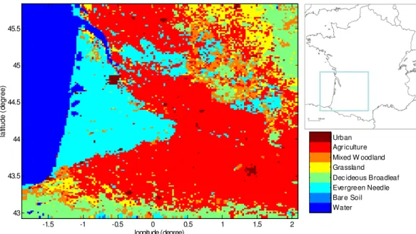
The area is characterized by several large areas of homogeneous land cover, with the Les Landes pine forest in the west, woods and pastures in the northeast, and large areas of cultivated plots in the rest of the domain (Fig. 1). Two major cities are located in the southeast (Toulouse) and northwest (Bordeaux) corners of the domain.

5

In this study two different days were simulated to compare the influence of different synoptic scale meteorology on the REs. The first day, 27 June 2005, was very warm with anti-cyclonic clear sky conditions. The wind came mainly from the southeast and allowed the formation of a sea breeze in the afternoon. On the second selected day, 6 June 2005, north-western winds prevailed. This day was cooler, and some cumulus

10

clouds formed in the afternoon in the northern part of the domain.

The two selected days were part of intensive observation periods within the CERES campaign. The simulations were compared to the available observations and the most important findings were described in the model intercomparison of 5 mesoscale models by Sarrat et al. (2007b). That comparison shows the ability of the models to represent

15

the atmospheric CO2 distribution satisfactory, in general agreement with the

observa-tions. They conclude that the complex spatial distribution as well as the temporal evo-lution of CO2in interaction with the surface fluxes are realistically simulated compared

to the aircrafts observations. Our model, B-RAMS performed satisfactory in most as-pects. Any possible further influences of discrepancies between the simulations and

20

the observations on the estimate of the RE are addressed in the discussion section. The surface fluxes in the standard simulations are calculated based on the Pelcom land use map with a homogeneous LAI per land use class (http://www.geo-informatie.

nl/projects/pelcom). To test the sensitivity of the RE to the formulation of the sur-face cover, land use maps derived from the Modis satellite data were used (http: 25

//modis-land.gsfc.nasa.gov/vi.htm), where the LAI can vary per pixel. Additionally, a simulation was performed in which a spatial homogeneous CO2 flux was prescribed

as a function of time. The prescribed maximal assimilation and respiration fluxes were about the average of the previously calculated maximal fluxes.

ACPD

Printer-friendly Version Interactive Discussion The standard simulations for the two days were thus kept very similar, i.e. with similar

land use maps and LAI and similar initialization of the CO₂concentration, so that the differences between the two days represent the influence of meteorology on the RE.

3 Results

Our simulations show that a number of processes contribute to the total RE, and their

5

relative contribution is different on both days simulated. REs are always associated with strong horizontal gradients in the CO₂ distribution. There are large variations across the spatial domain due to differences in land-surface type and topography. In the next sections, we will separately discuss each process contributing to the total RE, which spans a range from 0.5 ppm to as much 10 ppm. First, we will illustrate the dominant

10

mesoscale circulation patterns to provide appropriate background for the analysis.

3.1 Mesoscale circulations

The simulations show that the RE has a large spatial and temporal variability. The two simulated days show a clear distinction, where the REs during the day at 27 May exceeded those on 6 June. The largest difference between the two days is the synoptic

15

wind direction, which originates from the southeast at 27 May and from the west at 6 June. On 27 May mesoscale circulations formed, these were suppressed on 6 June. During the night of 27 May the south-eastern wind moved air with a high CO₂ con-centration, because of respiration, from the land over the sea. Since the CO2 fluxes

over the sea are relatively small the CO2 concentrations remain high there during the

20

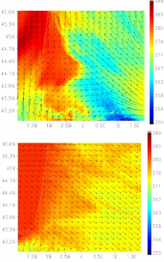
following day. In the course of the day a sea breeze developed. The direction of the sea breeze was at 27 May opposite to the synoptic wind direction. The converging winds led to the formation of a front (Fig. 2a). A gradient of about 10 ppm formed between the high nocturnal concentrations over the ocean and the depleted concentrations over the land perpendicular to the coast line. This was also described by Dolman et al. (2006),

ACPD

Printer-friendly Version Interactive Discussion Sarrat et al. (2007a) and Ahmadov et al. (2007).

Additionally, differences in vegetation types and corresponding sensible heat fluxes induced mesoscale circulations. The relatively high sensible heat flux above the forest resulted in a deep boundary layer compared to its surroundings. On 27 May the deep boundary layer was stationary over the forest due to the opposing wind directions,

5

strengthening the convection.

In contrast, on 6 June the synoptic wind was directed from sea to land and similar to the main direction of the sea breeze. Neither advection of the nocturnal high con-centrations from land to sea, nor the formation of a convergence zone during the day takes place (Fig. 2b). The effects of the sea breeze on the CO2concentration are thus

10

suppressed by the westerly wind on 6 June. Also, the high boundary layer over the forest is advected over the rest of the domain. This eliminates the strong contrast be-tween the depth of the boundary layer over the forest and its surroundings. At 6 June background CO₂concentrations from the ocean are advected over the land, where it is depleted due to CO2 uptake at the surface during the day. This causes a gradual

15

decreasing gradient in the CO2concentration land inward (Fig. 2b).

3.2 Representation errors due to mesoscale circulations

The large concentration contrasts over small distances induced by mesoscale circu-lations may lead to a large RE. On 6 June the gradual gradients and the absence of mesoscale circulation fronts cause a horizontal homogeneous spatial distribution of the

20

RE. On 27 May a higher RE is simulated than at 6 June (Fig. 3). At locations that are not affected by mesoscale circulations, the REs on 27 May are comparable to those observed at 6 June. The high RE on 27 May is located in grid cells in the vicinity of the edges of the convergence zone (Fig. 4). Near the front a RE of about 2.5 ppm is found at 10 km resolution, and about 5.5 ppm at 100 km resolution.

25

On 27 May, the depleted air from the boundary layer is elevated in the convergence zone, where it comes next to the free tropospheric air above the top of the boundary layer in the rest of the domain. This leads to a band with high REs along the eastern

ACPD

Printer-friendly Version Interactive Discussion edge of the convergence zone, which dominate the average RE over the domain. The

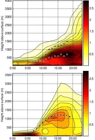
highest REs during the day are found around the top of the boundary layer (Fig. 5). Also in the rest of the domain and on 6 June the RE is high around the mean height of the top of the boundary layer (Fig. 5b). This is a result of the difference between convection cells and their surroundings, causing strong horizontal gradients between

5

the depleted boundary layer and free tropospheric air. On 6 June this effect stretches over a large vertical range (Fig. 5b). This is due to the formation of clouds and the consequent deep convection, causing horizontal variations in the CO₂ concentration up to 3000 m height during the day.

Above the sea the boundary layer is very shallow, and therefore the largest REs are

10

limited there to the lower part of the atmosphere. For example, the RE at 250m height as shown in Fig. 4 is small, since it is above the boundary layer. Within the boundary layer over the sea, the RE depends strongly on the wind direction. On 27 May the edges of air masses influenced by nocturnal land fluxes and transported from land during the night, causing high REs. The high concentrations from the land contrast here

15

with the background concentrations over the sea. On 6 June, the wind from overseas brings “background” air, which is not influenced by any strong near field terrestrial fluxes. The REs over most of the sea are therefore very small over the sea on 6 June. 3.3 Representation errors in the free troposphere

The free tropospheric RE is influenced by the CO2concentration gradients in the

resid-20

ual boundary layer (Fig. 5). Therefore, the differences between the two simulated days due to the meteorological circumstances extend out towards the evening and the night. During the first simulated nights the REs in the layers above the nocturnal boundary layer are underestimated, because of the lack of residual boundary layer since the CO₂ concentrations for both days are initialized homogeneous at 18:00 the previous day.

25

During the evening of 27 May, the convergence zone due to the sea breeze remains intact until the temperature of the land decreases towards the sea water temperature. Up to that moment, the boundary layer air is forced to rise to higher altitudes.

Com-ACPD

Printer-friendly Version Interactive Discussion bined with the influence of the upwind mountains, this leads to an ongoing increase in

the RE at higher altitudes (Fig. 5a).

Analyses of the RE for 6 June show that the RE in the residual boundary layer gradually decreases during the evening and the night (Fig. 5b). After the collapse of the boundary layer at the end of the day, the relative strong horizontal winds above

5

the nocturnal boundary layer cause mixing. This diminishes the horizontal variations in the CO2 concentration and thus the REs at altitudes that are no longer influenced by

the surface fluxes.

3.4 Representation errors due to topography

During the night the presence of the high mountains of the Pyrenees in the south of the

10

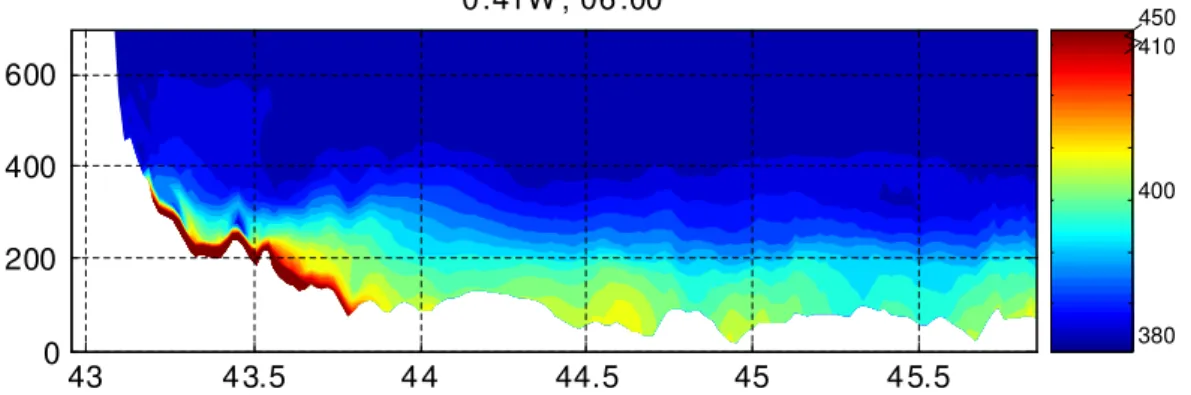
domain strongly influences the RE at lower altitudes. In the simulations for both days a band with high CO₂concentrations accumulates at the foot of the Pyrenees (Fig. 6). It strongly contrasts with the lower concentrations in the flatter areas and the tops of the mountains. This leads to a high RE near the surface during the night.

After sunrise, over the land the high CO₂ concentrations at the foot of the Pyrenees

15

are decreased due to the growth of the boundary layer and CO2uptake at the surface.

Over the sea, the high CO2concentrations are preserved in the shallow boundary layer

and lead to enhanced REs during the whole day.

Smaller scale topographic features also induce RE. During the night, accumulation of CO2 is simulated in valleys with up to a hundred meters altitude difference.

Fig-20

ure 6 shows the variations in the CO₂concentration at the end of the night, at 27 May 06:00 UTC, simulated with a spatially constant CO2 flux. These variations are thus

totally due to CO2 transport. The variations induced by small scale variations in the

surface altitude, remote of the Pyrenees, cause a RE of 0.5–3 ppm at 10 km resolution, and about 3 ppm at 100 km resolution. After sunrise, the gradients in the CO2

concen-25

trations formed during the night decrease, and consequently the representation error is reduced near the surface.

ACPD

Printer-friendly Version Interactive Discussion 3.5 Representation errors due to CO₂flux variability

The RE during the night hardly differs between the simulations with calculated and spa-tially homogeneous prescribed fluxes. CO₂flux variability thus appears unimportant in the nocturnal RE. During daytime, the REs simulated with a spatial homogeneous flux are only half as large as those of the standard simulation. The REs are reduced at all

5

heights within the boundary layer and at all resolutions addressed. Gradients caused by the surface CO2 flux extend over a large range of spatial scales. Blocks of

con-trasting vegetation types and accompanying concon-trasting CO2fluxes cause large scale

variations that may strengthen the effect of the mesoscale circulations. Ahmadov et al. (2007) showed the covariation (3-D-rectifier) between the mesoscale circulations

10

and these gradients as the surface flux responds to local weather. Additionally, the surface signal is advected in the direction of the main wind, and results in atmospheric stripes with different CO2 concentrations downwind of the surface flux variation.

Vari-ations in the surface CO2flux contribute at 100 km resolution up to 2 ppm to the total

RE during daytime and are thus an important contributor.

15

4 Discussion and conclusions

The RE of atmospheric CO2concentration at regional scales is found to be substantial.

It is a source of uncertainty that should be taken in account in inversion studies to avoid biased results. However, not a single constant number can be used, because of the heterogeneity in time and space. The order of magnitude of the RE above the

20

continent appears to be comparable to other sources of uncertainties like transport and rectification errors. The most important contribution to RE in our small domain during the day comes from surface flux variability and mesoscale transport phenomena such as the land-sea breeze. Our numbers are somewhat higher, but in the same order of magnitude as the REs estimated in the studies of Gerbig et al. (2003a, b) based on

25

ACPD

Printer-friendly Version Interactive Discussion study by Van der Molen and Dolman (2007) over Siberia.

The reliability of the estimates of the RE in this study was tested with a number of sensitivity tests. The conclusions in this work appeared not to depend on the initial CO₂concentration. The use of the Modis land use map instead of the Pelcom land use map (Table 1) did not change the main sources of REs. On 6 June, the boundary layer

5

height was simulated correctly compared to the observations. On 27 the boundary layer height was underestimated by the model at some locations (for details see Sarrat et al., 2007b). The strength of the vertical mixing determines the dilution of the surface signal in the atmosphere. Therefore, the occasional underestimation of the boundary layer depth may have led to a slight overestimation of the REs in this study.

10

The assumption that the simulation at 2 km resolution captures all variability in the CO2 concentration may on the other hand lead to an underestimation of the RE. The

variation caused by small scale eddies and variability in the CO2 fluxes at scales

smaller than 2 km are ignored in this study. The former are generally random, and are probably removed from observations by averaging the data over half an hour or

15

more. Flux variability at a scale smaller than 2 km may add some extra RE. The RE due to CO₂ flux variability as described in the result section is likely to extend over a large range of scales, including the fine scale.

Hence, the absolute values of the RE in this study must be handled with caution. The processes we found to cause the RE are robust and the difference of the RE between

20

the two days is larger than the sensitivity to the model settings. Therefore, it seems justified to use the simulations as a basis for a qualitative analysis of the RE.

Our work gives a suggestion for the reduction of REs. Within the boundary layer, the RE is lowest during the day in the well mixed part. This is thus the best location and time to get a representative sample. Observation locations close to the edges

25

of contrasting surface covers or elevation differences should be handled with caution, because mesoscale circulations may lead there to high REs. Observations around the top of the boundary layer should be avoided as the RE is high there.

ACPD

Printer-friendly Version Interactive Discussion breeze front caused by the sharp contrast between air masses with different flow

histo-ries. A correct interpretation of a CO₂ concentration observation as representative for air with a terrestrial footprint, in our simulations east of the front, or as representative for air within the sea breeze can vastly reduce the RE. The measured wind direction at the observation location, and a possible change in the observed CO₂concentration as the

5

sea breeze reaches the observation location, may indicate the origin of the measured air mass. In transport models the location of the front may not be simulated entirely correct, due to transport errors or coarse resolutions. Reinterpretation of the sampling location in the model for such an observation may help to reduce the RE.

At night, topography is the main source of REs. The simulated accumulation of CO2

10

in the valleys is in line with the findings of previous model (Nicholls et al., 2004; Van der Molen and Dolman, 2007) and observational studies (Eugster and Siegrist, 2000; Ara ´ujo et al., in preparation; Goulden et al., 2006; Aubinet et al., 2003) which show that near surface cooling leads to katabatic drainage flow of CO₂ rich air. Nocturnal observations at high mountains may after data selection be taken as representative of

15

the CO2concentration at their height above sea level (e.g. Schmidt et al., 2003; Geels

et al., 2007) with accompanying relatively low free tropospheric REs.

Katabatic drainage due to small scale topography of up to 100 m altitude leads to concentration gradients within the nocturnal boundary layer (Fig. 6). Concentrations in the valleys are enhanced by accumulation of respired CO₂, while concentrations at

20

higher parts are reduced. Consequently, when an observation that is taken in a valley is assumed to be representative for a larger area, including higher parts, the average CO₂ concentration will be overestimated for that area. Observations on high parts will conversely lead to a systematic underestimation of the real CO2concentration. In

our simulations the accumulated CO2 concentration was seen to be advected by the

25

dominant winds, which may further complicate the interpretation of CO₂concentration observations. Therefore, if nocturnal CO2 concentrations are regarded important it is

advisable to avoid locations close to river valleys and hills and the foot of large scale topographic features. Otherwise, near these features REs of up to about 3 ppm should

ACPD

Printer-friendly Version Interactive Discussion be taken in account.

Further, increasing the number of observations to achieve a better constraint on the mean CO2 concentration can reduce the RE. The required accuracy of the

observa-tions depends on the resolution at which the REs will be interpreted. Our simulaobserva-tions indicate that even at a relatively high resolution (10 km) the RE over the land exceeds

5

the error introduced by the measurement accuracy aimed for at high accuracy sta-tions. Extra towers can thus give a better constraint on the average CO2concentration.

To reduce the RE an observation network with a number of clustered towers may be favourable over a regularly spaced network. The ring of towers around the WLEF tower is an example of such a tower cluster (Zupanski et al., 2007), which may be applied at

10

smaller scales too.

Obviously, increasing the model resolution is the most straight forward manner of decreasing the RE. How much the resolution must be increased to resolve the main CO₂concentration variability depends on the strength and the horizontal extent of the surface CO2 flux variability and the meteorology. Since variations in CO2

concentra-15

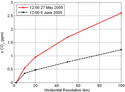
tion are present at all scales, increasing the resolution always leads to a reduction of the RE. The results of this study suggest that much can be gained when increasing the resolution from relative coarse scales of 100 km toward finer resolutions (Fig. 3), especially when large scale phenomena like the sea breeze cause contrasts in the CO2concentration. To reduce the RE due to small scale variability the largest gain

20

is obtained when the resolution is increased to finer scales than 10 km. An optimum resolution must be found considering additionally computational expenses, input data availability, model parameterizations, etcetera. Alternatively, one may consider nesting a high resolution grid around a high accuracy observation within the coarser simulation to reduce REs and to preserve most of the information in the observation.

25

We conclude that REs in tracer transport modelling can be considerable and need to be taken into account. High REs are simulated in the nocturnal boundary layer caused by topography. These may lead to systematic errors in the estimation of the mean CO2

ACPD

Printer-friendly Version Interactive Discussion and low resolution simulations. Additionally, mesoscale circulations may give rise to

high REs, and observations must therefore be scaled up carefully. If observations are associated with the proper influence history, our simulations suggest that the RE in the boundary layer during the afternoon can be limited to below 1 ppm up to at least 20 km resolution, or a coarser resolution when the circumstances are favourable like in this

5

study at 6 June.

Acknowledgements. This work has been done in the framework of the Dutch project

“Cli-mate changes Spatial Planning”, BSIK-ME2 and the Carboeurope Regional Component (GOCE CT2003 505572). We thank the CERES participants for discussions and making their observations available. Thanks to P. Rayner and S. Denning for their lessons and discussions

10

on inverse CO₂modelling.

References

Ahmadov, R., Gerbig, C., Kretschmer, R., Koerner, S., Neininger, B., Dolman, A., and Sarrat, C.: Mesoscale covariance of transport and CO₂ fluxes: Evidence from observations and simulations using the wrf-vprm coupled atmosphere-biosphere model, J. Geophys. Res, 112,

15

D22107, doi:10.1029/2007JD008552, 2007.

Ara ´ujo de, A. C., Kruijt, B., Nobre, A. D., Dolman, A. J., Waterloo, M. J., Moors, E. J., and Souza de, J. S.: Nocturnal accumulation of CO₂underneath a tropical forest canopy along a topographical gradient, Ecol. Appl., in press, 2008.

Aubinet, M., Heinesch, B., and Yernaux, M.: Horizontal and vertical CO₂advection in a sloping

20

forest, Bound.-Lay. Meteorol., 108, 397–417, 2003.

Baker, D. F., Law, R. M., Gurney, K. R., Rayner, P., Peylin, P., Denning, A. S., Bousquet, P., Bruhwiler, L., Chen, Y. H., Ciais, P., Fung, I. Y., Heimann, M., John, J., Maki, T., Maksyu-tov, S., Masarie, K., Prather, M., Pak, B., Taguchi, S., and Zhu, Z.: Transcom 3 inversion intercomparison: Impact of transport model errors on the interannual variability of regional

25

CO₂fluxes, 1988–2003, Global Biogeochem. Cy., 20, GB1002, doi:10.1029/2004GB002439, 2006.

ACPD

Printer-friendly Version Interactive Discussion

atmospheric CO₂ sources and sinks 1. Method and control inversion, J. Geophys. Res.-Atmos., 104, 26 161–26 178, 1999.

Carouge, C.: Vers une estimation des flux de CO₂europeen, 2006.

Denning, A. S., Randall, D. A., Collatz, G. J., and Sellers, P. J.: Simulations of terrestrial carbon metabolism and atmospheric CO₂in a general circulation model: 2. Simulated CO₂

5

concentrations, Tellus Series B-Chemical and Physical Meteorology, 48, 543–567, 1996. Denning, A. S., Nicholls, M., Prihodko, L., Baker, I., Vidale, P. L., Davis, K., and Bakwin, P.:

Sim-ulated variations in atmospheric CO₂ over a Wisconsin forest using a coupled ecosystem-atmosphere model, Glob. Change Biol., 9, 1241–1250, 2003.

Dolman, A. J., Noilhan, J., Durand, P., Sarrat, C., Brut, A., Piguet, B., Butet, A., Jarosz, N.,

10

Brunet, Y., Loustau, D., Lamaud, E., Tolk, L., Ronda, R., Miglietta, F., Gioli, B., Magliulo, V., Esposito, M., Gerbig, C., Korner, S., Glademard, R., Ramonet, M., Ciais, P., Neininger, B., Hutjes, R. W. A., Elbers, J. A., Macatangay, R., Schrems, O., Perez-Landa, G., Sanz, M. J., Scholz, Y., Facon, G., Ceschia, E., and Beziat, P.: The Carboeurope regional experiment strategy, B. Am. Meteorol. Soc., 87, 1367–1379, 2006.

15

Eugster, W. and Siegrist, F.: The influence of nocturnal CO₂advection on CO₂flux measure-ments, Basic Appl. Ecol., 1, 177–188, 2000.

Fan, S., Gloor, M., Mahlman, J., Pacala, S., Sarmiento, J., Takahashi, T., and Tans, P.: A large terrestrial carbon sink in north america implied by atmospheric and oceanic carbon dioxide data and models, Science, 282, 442–446, 1998.

20

Farquhar, G. D., Caemmerer, S. V., and Berry, J. A.: A biochemical-model of photosynthetic CO₂assimilation in leaves of C-3 species, Planta, 149, 78–90, 1980.

Geels, C., Gloor, M., Ciais, P., Bousquet, P., Peylin, P., Vermeulen, A. T., Dargaville, R., Aalto, T., Brandt, J., Christensen, J. H., Frohn, L. M., Haszpra, L., Karstens, U., Rodenbeck, C., Ramonet, M., Carboni, G., and Santaguida, R.: Comparing atmospheric transport models

25

for future regional inversions over europe - part 1: Mapping the atmospheric CO₂ signals, Atmos. Chem. Phys., 7, 3461–3479, 2007,

http://www.atmos-chem-phys.net/7/3461/2007/.

Gerbig, C., Lin, J. C., Wofsy, S. C., Daube, B. C., Andrews, A. E., Stephens, B. B., Bakwin, P. S., and Grainger, C. A.: Toward constraining regional-scale fluxes of CO₂with atmospheric

30

observations over a continent: 1. Observed spatial variability from airborne platforms, J. Geophys. Res.-Atmos., 108(D24), 4756, doi:10.1029/2002JD003018, 2003a.

ACPD

Printer-friendly Version Interactive Discussion

S., and Grainger, C. A.: Toward constraining regional-scale fluxes of CO₂with atmospheric observations over a continent: 2. Analysis of cobra data using a receptor-oriented framework, J. Geophys. Res.-Atmos., 108(D24), 4757, doi:10.1029/2003JD003770, 2003b.

Goulden, M. L., Miller, S. D., and da Rocha, H. R.: Nocturnal cold air drainage and pooling in a tropical forest, J. Geophys. Res.-Atmos., 111, D08S04, doi:10.1029/2005JD006037, 2006.

5

Gurney, K. R., Law, R. M., Denning, A. S., Rayner, P. J., Baker, D., Bousquet, P., Bruhwiler, L., Chen, Y. H., Ciais, P., Fan, S., Fung, I. Y., Gloor, M., Heimann, M., Higuchi, K., John, J., Maki, T., Maksyutov, S., Masarie, K., Peylin, P., Prather, M., Pak, B. C., Randerson, J., Sarmiento, J., Taguchi, S., Takahashi, T., and Yuen, C. W.: Towards robust regional estimates of CO₂ sources and sinks using atmospheric transport models, Nature, 415, 626–630, 2002.

10

Houweling, S., Dentener, F., Lelieveld, J., Walter, B., and Dlugokencky, E.: The modeling of tropospheric methane: How well can point measurements be reproduced by a global model?, J. Geophys. Res.-Atmos., 105, 8981–9002, 2000.

Kaminski, T., Rayner, P. J., Heimann, M., and Enting, I. G.: On aggregation errors in atmo-spheric transport inversions, J. Geophys. Res.-Atmos., 106, 4703–4715, 2001.

15

Karstens, U., Gloor, M., Heimann, M., and Rodenbeck, C.: Insights from simulations

with high-resolution transport and process models on sampling of the atmosphere for constraining midlatitude land carbon sinks, J. Geophys. Res.-Atmos., 111, D12301, doi:10.1029/2005JD006278, 2006.

Lauvaux, T., Uliasz, M., Sarrat, C., Chevallier, F., Bousquet, P., Lac, C., Davis, K. J., Ciais, P.,

20

Denning, A. S., and Rayner, P. J.: Mesoscale inversion: First results from the ceres campaign with synthetic data, Atmos. Chem. Phys. Discuss., 7, 10 439–10 465, 2007.

Lin, J. C., Gerbig, C., Daube, B. C., Wofsy, S. C., Andrews, A. E., Vay, S. A., and An-derson, B. E.: An empirical analysis of the spatial variability of atmospheric CO₂: Impli-cations for inverse analyses and space-borne sensors, Geophys. Res. Lett., 31, L23104,

25

doi:10.1029/2004GL020957, 2004.

Medvigy, D., Moorcroft, P. R., Avissar, R., and Walko, R. L.: Mass conservation and atmo-spheric dynamics in the regional atmoatmo-spheric modeling system (RAMS), Environmental Fluid Mechanics, 5, 109-134, 2005.

Nicholls, M. E., Denning, A. S., Prihodko, L., Vidale, P. L., Baker, I., Davis, K., and

30

Bakwin, P.: A multiple-scale simulation of variations in atmospheric carbon dioxide us-ing a coupled biosphere-atmospheric model, J. Geophys. Res.-Atmos., 109, D18117, doi:10.1029/2003JD004482, 2004.

ACPD

Printer-friendly Version Interactive Discussion

Perez-Landa, G., Ciais, P., Gangoiti, G., Palau, J. L., Carrara, A., Gioli, B., Miglietta, F., Schu-macher, M., Millan, M. M., and Sanz, M. J.: Mesoscale circulations over complex terrain in the Valencia coastal region, Spain – part 2: Modeling CO₂transport using idealized surface fluxes, Atmos. Chem. Phys., 7, 1851–1868, 2007,

http://www.atmos-chem-phys.net/7/1851/2007/.

5

Peters, W., Krol, M. C., Dlugokencky, E. J., Dentener, F. J., Bergamaschi, P., Dutton, G., von Velthoven, P., Miller, J. B., Bruhwiler, L., and Tans, P. P.: Toward regional-scale modeling using the two-way nested global model TM5: Characterization of transport using SF₆, J. Geophys. Res.-Atmos., 109, D19314, doi:10.1029/2004JD005020, 2004.

Peters, W., Jacobson, A., Sweeney, C., Andrews, A., Conway, T., Masarie, K., Miller, J.,

Bruh-10

wiler, L., Petron, G., and Hirsch, A.: An atmospheric perspective on North American carbon dioxide exchange: Carbontracker, Proceedings of the National Academy of Sciences, 104, 18 925–18 930, 2007.

Pielke, R. A., Cotton, W. R., Walko, R. L., Tremback, C. J., Lyons, W. A., Grasso, L. D., Nicholls, M. E., Moran, M. D., Wesley, D. A., Lee, T. J., and Copeland, J. H.: A comprehensive

me-15

teorological modeling system - RAMS, Meteorology and Atmospheric Physics, 49, 69-91, 1992.

Rodenbeck, C., Houweling, S., Gloor, M., and Heimann, M.: CO₂ flux history 1982–2001

inferred from atmospheric data using a global inversion of atmospheric transport, Atmos. Chem. Phys., 3, 1919–1964, 2003,

20

http://www.atmos-chem-phys.net/3/1919/2003/.

Sarrat, C., Noilhan, J., Lacarrere, P., Donier, S., Lac, C., Calvet, J. C., Dolman, A. J., Gerbig, C., Neininger, B., Ciais, P., Paris, J. D., Boumard, F., Ramonet, M., and Butet, A.: Atmospheric CO₂modeling at the regional scale: Application to the carboeurope regional experiment, J. Geophys. Res.-Atmos., 112, D12105, doi:10.1029/2006JD008107, 2007.

25

Sarrat, C., Noilhan, J., Dolman, A. J., Gerbig, C., Ahmadov, R., Tolk, L. F., Meesters, A. G. C. A., Hutjes, R. W. A., Ter Maat, H. W., P ´erez-Landa, G., and Donier, S.: Atmospheric CO₂ modeling at the regional scale: An intercomparison of 5 meso-scale atmospheric models, Biogeosciences, 4, 1115–1126, 2007,

http://www.biogeosciences.net/4/1115/2007/.

30

Schmidt, M., Graul, R., Sartorius, H., and Levin, I.: The schauinsland CO₂record: 30 years of continental observations and their implications for the variability of the european CO₂budget, J. Geophys. Res.-Atmos., 108(D19), 4619, doi:10.1029/2002JD003085, 2003.

ACPD

Printer-friendly Version Interactive Discussion

Sellers, P. J., Los, S. O., Tucker, C. J., Justice, C. O., Dazlich, D. A., Collatz, G. J., and Randall, D. A.: A revised land surface parameterization (SiB2) for atmospheric GCMs. 2. The gener-ation of global fields of terrestrial biophysical parameters from satellite data, J. Climate, 9, 706–737, 1996.

Stephens, B. B., Gurney, K. R., Tans, P. P., Sweeney, C., Peters, W., Bruhwiler, L., Ciais, P.,

5

Ramonet, M., Bousquet, P., Nakazawa, T., Aoki, S., Machida, T., Inoue, G., Vinnichenko, N., Lloyd, J., Jordan, A., Heimann, M., Shibistova, O., Langenfelds, R. L., Steele, L. P., Francey, R. J., and Denning, A. S.: Weak northern and strong tropical land carbon uptake from vertical profiles of atmospheric CO₂, Science, 316, 1732–1735, 2007.

Van der Molen, M. K. and Dolman, A. J.: Regional carbon fluxes and the effect of

to-10

pography on the variability of atmospheric CO₂, J. Geophys. Res.-Atmos., 112, D01104, doi:10.1029/2006JD007649, 2007.

Van Dijk, A., and Dolman, A. J.: Estimates of CO₂uptake and release among european forests based on eddy covariance data, Glob. Change Biol., 10, 1445–1459, 2004.

Walko, R. L., Band, L. E., Baron, J., Kittel, T. G. F., Lammers, R., Lee, T. J., Ojima, D., Pielke, R.

15

A., Taylor, C., Tague, C., Tremback, C. J., and Vidale, P. L.: Coupled atmosphere-biophysics-hydrology models for environmental modeling, J. Appl. Meteorol., 39, 931–944, 2000. Wullschleger, S. D.: Biochemical limitations to carbon assimilation in C₃plants -a retrospective

analysis of the a/ci curves from 109 species, J. Exp. Bot., 44, 907–920, 1993.

Yang, Z., Washenfelder, R. A., Keppel-Aleks, G., Krakauer, N. Y., Randerson, J. T., Tans, P.

20

P., Sweeney, C., and Wennberg, P. O.: New constraints on northern hemisphere growing season net flux, Geophys. Res. Lett., 34, L12807, doi:10.1029/2007GL029742, 2007. Zupanski, D., Denning, A. S., Uliasz, M., Zupanski, M., Schuh, A. E., Rayner, P. J., Peters, W.,

and Corbin, K. D.: Carbon flux bias estimation employing maximum likelihood ensemble filter (MLEF), J. Geophys. Res.-Atmos., 112, D17107, doi:10.1029/2006JD008371, 2007.

ACPD

Printer-friendly Version Interactive Discussion

Table 1. Simulation specifications. Where two options are mentioned the second is used for sensitivity tests.

Atmospheric model Brams-3.2

Vegetation model Leaf-3

CO₂flux model Farquhar model

Turbulence scheme Mellor Yamada

Simulation setup:

Nesting Two way nested

Domain, resolution 300×300 km, 2 km; 1200×1200 km, 10 km

Domain centre 44.4 N, 0.1 W

Initial conditions:

Meteorology, ECMWF ERA40 reanalysis dataset

Soil moisture and Temperature (http://www.ecmwf.int)

CO₂concentration 1. Homogeneous 382 ppm

2. 375 ppm below, 382 above 1000 m Boundary conditions:

Meteorology 6 hourly nudged to ECMWF data

CO₂concentration Zero gradient

Surface Characteristics:

Land use 1. Pelcom database

(http://www.geo-informatie.nl/projects/pelcom) 2. Modis biomes and LAI

(http://modis-land.gsfc.nasa.gov/vi.htm)

Topography USGS dataset

(http://www.atmet.com)

Soil textural class UN FAO dataset

(http://www.atmet.com)

Fossil fuel emissions IER database

ACPD

Printer-friendly Version Interactive Discussion

Water Bar e Soil Evergreen Needle Dec ideous Broadleaf Grassland Mixed W oodland Agr iculture Urban la tit u d e ( d e g re e ) longitude (degree) -1.5 -1 -0.5 0 0.5 1 1.5 2 43 43.5 44 44.5 45 45.5

Fig. 1. Simulation domain and land use in southwest France. The domain is bounded in the west by the Atlantic Ocean and in the south by the Pyrenees.

ACPD

Printer-friendly Version Interactive Discussion

Fig. 2. CO₂ concentration in ppm and wind speed and direction at 250 m agl at 14:00 UTC,

27 May 2005 (a) and 6 June 2005 (b). The opposing wind directions on 27 May lead to large CO₂concentration gradients which are absent on 6 June.

ACPD

Printer-friendly Version Interactive Discussion

Fig. 3. Domain average RE at 250m above the surface for 12:00 at 27 May 2005 (red) and 12:00 at 6 June (black). This shows the increase of the RE with decreasing resolution, and the higher RE when mesoscale circulations are important at 27 May.

ACPD

Printer-friendly Version Interactive Discussion

Fig. 4. Spatial distribution of the RE [ppm] at 10 km resolution; 250 m above the surface at 14:00 UTC 27 May 2005. Blue indicates sea and green land. The highest REs are located near the edge of the mesoscale circulation front.

ACPD

Printer-friendly Version Interactive Discussion H e ig h t a b o v e s u rf a ce ( m ) 0:00 5:00 10:00 15:00 20:00 500 1000 1500 2000 2500 3000 3500 4000 0.5 1 1.5 2 2.5 H e ig h t a b o v e s u rf a ce ( m ) 0:00 5:00 10:00 15:00 20:00 500 1000 1500 2000 2500 3000 3500 0.5 1 1.5 2 2.5

Fig. 5. Variations of the representation errors at 27 May 2005 (a) and 6 June 2005 (b) with time and altitude. The representation errors are averaged over the area north of 44.16◦_N.

The circles in (a) indicate the height of the boundary layer in the convergence zone and the triangles the main boundary layer height over the rest of the land area at 27 May, in (b) the circles represent the more homogeneous main boundary layer height over the land at 6 June.

ACPD

Printer-friendly Version Interactive Discussion 0 .41W , 06 :00 43 4 3.5 4 4 44.5 45 4 5.5 0 200 400 600 380 400 410 450

Fig. 6. South-North vertical crosscut of the CO₂concentration in ppm at 27 May 06:00 UTC at 0.41◦_{W, simulated with a spatially constant CO}

2 flux. The concentrations between 43.3◦ and

43.8◦_{N, at the foot of the Pyrenees (on the left of figure), reach 450 ppm. Relative high CO2}

concentrations are also seen in the valleys of the Garonne river (44.6◦_{N) and the Dordogne}