HAL Id: hal-00330098
https://hal.archives-ouvertes.fr/hal-00330098
Submitted on 22 Nov 2006
HAL is a multi-disciplinary open access
archive for the deposit and dissemination of
sci-entific research documents, whether they are
pub-lished or not. The documents may come from
teaching and research institutions in France or
abroad, or from public or private research centers.
L’archive ouverte pluridisciplinaire HAL, est
destinée au dépôt et à la diffusion de documents
scientifiques de niveau recherche, publiés ou non,
émanant des établissements d’enseignement et de
recherche français ou étrangers, des laboratoires
publics ou privés.
kilometric radiation
U. Taubenschuss, H. O. Rucker, W. S. Kurth, B. Cecconi, P. Zarka, M. K.
Dougherty, J. T. Steinberg
To cite this version:
U. Taubenschuss, H. O. Rucker, W. S. Kurth, B. Cecconi, P. Zarka, et al.. Linear prediction studies for
the solar wind and Saturn kilometric radiation. Annales Geophysicae, European Geosciences Union,
2006, 24 (11), pp.3139-3150. �hal-00330098�
www.ann-geophys.net/24/3139/2006/ © European Geosciences Union 2006
Annales
Geophysicae
Linear prediction studies for the solar wind and Saturn kilometric
radiation
U. Taubenschuss1, H. O. Rucker1, W. S. Kurth2, B. Cecconi2, P. Zarka3, M. K. Dougherty4, and J. T. Steinberg5
1Space Research Institute, Austrian Academy of Sciences, A-8042 Graz, Austria
2Department of Physics and Astronomy, The University of Iowa, Iowa City, Iowa 52242, USA
3Laboratoire d’Etudes Spatiales et d’Instrumentation en Astrophysique, Observatoire de Paris, 92195 Meudon, France 4Blackett Laboratory, Imperial College of Science and Technology, London SW7 2BZ, UK
5Los Alamos National Laboratory, Los Alamos, New Mexico 87545, USA
Received: 4 April 2006 – Revised: 8 September 2006 – Accepted: 13 October 2006 – Published: 22 November 2006
Abstract. The external control of Saturn kilometric radiation (SKR) by the solar wind has been investigated in the frame of the Linear Prediction Theory (LPT). The LPT establishes a linear filter function on the basis of correlations between in-put signals, i.e. time profiles for solar wind parameters, and output signals, i.e. time profiles for SKR intensity. Three dif-ferent experiments onboard the Cassini spacecraft (RPWS, MAG and CAPS) yield appropriate data sets for compiling the various input and output signals. The time period investi-gated ranges from DOY 202 to 326, 2004 and is only limited due to limited availability of CAPS plasma data for the so-lar wind. During this time Cassini was positioned mainly on the morning side on its orbit around Saturn at low southern latitudes. Four basic solar wind quantities have been found to exert a clear influence on the SKR intensity profile. These quantities are: the solar wind bulk velocity, the solar wind ram pressure, the magnetic field strength of the interplane-tary magnetic field (IMF) and the y-component of the IMF. All four inputs exhibit nearly the same level of efficiency for the linear prediction indicating that all four inputs are pos-sible drivers for triggering SKR. Furthermore, they act at completely different lag times ranging from ∼13 h for the ram pressure to ∼52 h for the bulk velocity. The lag time for the magnetic field strength is usually beyond ∼40 h and the lag time for the y-component of the magnetic field is located around 30 h. Considering that all four solar wind quantities are interrelated in a corotating interaction region, only the influence of the ram pressure seems to be of reasonable rele-vance. An increase in ram pressure causes a substantial com-pression of Saturn’s magnetosphere leading to tail collapse, injection of hot plasma from the tail into the outer magneto-sphere and finally to an intensification of auroral dynamics and SKR emission. So, after the onset of magnetospheric
Correspondence to: U. Taubenschuss
compression at least ∼1.2 rotations of the planet elapse until intensified SKR emission is visible in a Cassini-RPWS dy-namic spectrum.
Keywords. Magnetospheric physics (Solar wind-magnetosphere interactions) – Radio science (Magne-tosphere physics; Radio astronomy)
1 Introduction
Before the launch of the Cassini spacecraft, the knowledge of Saturn’s radio emitting properties was based on data gained by the Voyager 1 and 2 missions (Warwick et al., 1981, 1982) and by the Ulysses spacecraft (Lecacheux et al., 1997).
The Saturn kilometric radiation (SKR) was detected for the first time when Voyager 1 was approaching Saturn in 1980 (Kaiser et al., 1980). This nonthermal radio emis-sion usually occurs in the frequency range 3 kHz−1.2 MHz with a broad peak in flux density between 100−400 kHz (Kaiser et al., 1984). The maximum flux density is at
∼3×10⁻¹⁹Wm−2Hz−1 normalized to a distance of 1 AU
to the planet. The spectrum typically looks bursty includ-ing also arc-like structures and bands and, accordinclud-ing to re-cent Cassini observations, also fine structures if analyzed with time resolutions in the millisecond regime (Kurth et al., 2005b). Two components of opposite senses of nearly 100% circular polarization have been identified which propagate as X-mode waves. Radiation coming from the northern hemi-sphere is right-handed polarized (RH) and radiation coming from the southern hemisphere is left-handed polarized (LH). Similar to radio wave phenomena observed at Earth and Jupiter, the Cyclotron Maser Instability (CMI) is an appro-priate model for explaining the generation of SKR, too (Wu and Lee, 1979). The CMI theory describes the generation
of planetary radio waves on the basis of a kinetic instability driven by a loss cone distribution for electron velocities.
The source regions of SKR are located in high magnetic northern and southern latitudes along auroral magnetic field lines. They are centered with respect to 13:00 LT near the noon meridian of Saturn above 80◦latitude. On the morning side between 08:00–09:00 LT possible source regions range down to 60◦ latitude and on the evening side at 19:00 LT sources down to 75◦ are possible (Galopeau et al., 1995). UV observations of bright aurora phenomena performed with the Hubble Space Telescope (HST) confirm the presence of energetic auroral electrons in the morning-to-noon sector (Trauger et al., 1998). Furthermore, HST observations show a nearly continuous UV auroral oval around the magnetic pole (Clarke et al., 2005) justifying the existence of SKR emission emitted from the nightside of Saturn as reported recently by Farrell et al. (2005).
Correlation studies between variations of the solar wind and SKR emission were published by Desch (1982) for the first time. He found clear correlations between the solar wind ram pressure ρ v2(mass density ρ, bulk velocity v) and SKR intensity in Voyager 1 and 2 data sets. A further indication of the strong dependence of SKR activity on the solar wind was found by Desch (1983). He detected a total disappearance of SKR during times when Saturn was moving through distant filaments of Jupiter’s magnetotail and was thus shielded from the solar wind. Later on, Desch and Rucker (1983, 1985) im-proved those correlation studies using the superposed epoch method and a compilation of various solar wind quantities. They came to the conclusion that besides the ram pressure the solar wind momentum (ρ v) and the kinetic energy (ρ v3) are also significant drivers for triggering SKR. The highest correlation coefficients have been found at zero lag time with a time resolution of 10.66 h, i.e. data have been integrated over one full rotation period of Saturn. The interplanetary magnetic field (IMF) and its components revealed no clear correlation with SKR which may be due to the fact that so-lar wind measurements were performed up to 1.6 AU ahead of Saturn and had to be ballistically propagated to the point of the planet thereby ignoring hydrodynamic interactions of high- and low-speed streams inside the solar wind.
The solar wind exerts its external control not only on SKR generation but also on Saturn’s aurorae as investigated re-cently by Clarke et al. (2005) and Crary et al. (2005). New Cassini data in combination with ground-based and HST ob-servations related Saturn’s radio emission phenomena to de-tailed auroral structures (Kurth et al., 2005a).
The present paper re-analyses the external control of SKR by the solar wind with the application of the Linear Predic-tion Theory, outlined in Sect. 2. The data used as input and output time series are described in Sect. 3. The results are presented in Sect. 4 and the final Sect. 5 comprises the dis-cussion and conclusion.
2 Basics of the Linear Prediction Theory
The Linear Prediction Theory (LPT) was developed by the American mathematician N. Wiener (Wiener, 1949), at first for continuous time series, and later on adapted by Levinson (1949) to discrete time series. The main aim of the LPT is to predict a function Y , called output signal, by convolving a filter function f with another function X, called the input signal. For the discrete case the convolution equation looks like the following:
Yt = M−1
X
s=−m
fsXt −s. (1)
A certain value Yt of the output is calculated by
multiply-ing the filter coefficients fs with a sample of input data Xt −s
and then summing these weighted input data. If Xt and Yt
are time series representations then index t indicates a cer-tain time and index s indicates the temporal shift or lag. A summation using only positive s-indices (s=0, . . . , M−1) is called the causal part of the filtering because only in-put data from the past are considered. Negative s-indices (s= −m, . . . , −1) contribute to the acausal part of the fil-tering which causes a physical conflict because it calculates output data taking input data from the future, i.e. an effect would precede the cause. Nevertheless, it could become im-portant to calculate the acausal part too, especially for ex-plaining strong filter reactions around lag position zero or to test the significance of a causal relationship.
The LPT works exclusively with a non-recursive filter as outlined in Eq. (1) and furthermore, the filter has to be linear and time invariant. Additionally, the time series used must be sampled from a stochastic process and the time series must be stationary.
The Linear Prediction Theory is usually applied on the condition that the input signal Xt and the measured output
signal Zt are known by means of corresponding
measure-ments and that the filter coefficients fshave to be calculated.
The measured output is named Zt in order to distinguish it
from the calculated output Yt. The filter fs must be
consti-tuted such that Yt becomes the best possible representation
of Zt as far as their linear relationship is concerned. So, the
mean-square-error between Zt and Yt has to be minimized.
Stressing the convolution equation in combination with the statistical criteria of least squares fitting makes a calculation of the filter coefficients possible. The relationships between input, outputs and filter are sketched in Fig. 1.
The procedure for calculating the filter coefficients of a single-channel filter is presented in the Appendix. As a last step, the filter coefficients together with the input Xt have
to be inserted into the convolution equation (1) to get the calculated output signal Yt.
A parameter for quantifying the degree of fit between the calculated output Ytand the measured output Zt, i.e. the
per-formance of the linear prediction, is the efficiency defined as
eff = 1 −σ 2 r σ2 z ! × 100 [%] . (2)
σz2is the variance of Zt and σr2is the variance of the
resid-ual time series (Zt−Yt). An efficiency of +100% means that
all variations of the measured output Zt are reproduced by
the variations of the calculated output Yt. On the other hand,
a negative value for eff indicates that Yt does not reproduce
the variations of Zt and hence the prediction of the output
Zt by the input Xt is wrong. Moreover, the efficiency can
be investigated as a function of the temporal shift parameter
s. Therefore, the output Yt has to be calculated with a
suc-cessively increasing maximum shift. The filtering process is said to be completed if an additional extension of the filter does not raise the efficiency any more.
Finally, some further important remarks on the LPT are given. It is important that the signals which are applied to the LPT analysis contain the same number of discrete data points and exhibit the same time resolution. Thus, the signals must comprise the same time period. Furthermore, the maximum allowed number of discrete shifts, i.e. (M+m), is limited to 15% of the overall number N of data points (Taubenheim, 1969; Sch¨onwiese, 1985).
An exact representation of the measured output Zt by the
calculated output Yt is only possible if the summation in
Eq. (1) is performed from negative infinity to positive infinity and if the relation is strictly linear and time invariant. These conditions can hardly be fulfilled by real measured signals and one has to accept the fact that only a certain level of efficiency lower than 100% will be achieved. So, the disad-vantage of the LPT is the fact that it ignores relations hav-ing higher moments of the investigated process. Moreover, a filter is only valid for the time period selected for the cal-culations. On the other hand, it simplifies the analysis as a first approximation by assuming a linear system. Even if the relation between the input and output is not strictly linear, the Linear Prediction Theory will calculate the best possible linear relation.
The scenario described above using one measured input and one measured output is called single-channel system. As an extension, a so-called multi-channel system operates with more than one input and output. If the LPT is car-ried out in multi-channel mode, all signals will be processed collectively, thereby not ignoring relations among the indi-vidual signals. The computation of the filter coefficients follows the same concept as outlined in the appendix for the single-channel system except that cross-correlation and auto-correlation coefficients have to be arranged in tensors of higher dimension. measured input Xt fs calculated output Yt measured output Zt minimize error
Fig. 1. Schematics of the concepts of the Linear Prediction Theory.
The measured input Xtis filtered (filter function fs) yielding a cal-culated output Yt which is then compared to the actually measured output Zt. The error power between Ytand Ztshall be minimized.
3 Preparation of input and output signals
The Linear Prediction Theory was used to investigate the in-fluence of the solar wind on SKR intensity. Profiles for vari-ous solar wind quantities serve as input signals and SKR in-tegrated intensity-time profiles serve as output signals. Data obtained by three different experiments onboard the Cassini spacecraft have been used to construct input and output sig-nals feeding the LPT algorithm. These three experiments are the Radio and Plasma Wave Science experiment (RPWS) (Gurnett et al., 2004), the Dual Technique Magnetometer (MAG) (Dougherty et al., 2004) and the Cassini Plasma Spectrometer (CAPS) (Young et al., 2004).
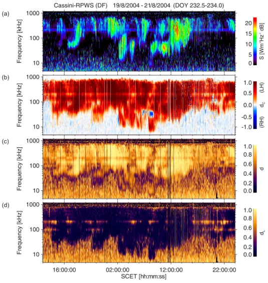
SKR intensity profiles are established using data from the RPWS experiment. One important point is that these pro-files use only SKR emissions. SKR emissions can be clearly identified in a dynamic spectrum regarding the frequency range and the polarization characteristics. SKR usually oc-curs in the frequency range 3−1200 kHz and exhibits a high degree of circular polarization (nearly 100%). The polariza-tion of measured radio waves was determined by applying the Direction-Finding algorithm for a 3-axis stabilized space-craft using a direct inversion (Cecconi and Zarka, 2005a). The Direction-Finding analysis yields not only the full po-larization information of the received radio waves, i.e. the Stokes parameters, but also eliminates the influence of in-tensity variations which are due to a changing orientation of the antenna system with regard to the direction of the radio source. Figure 2 demonstrates the results of the Direction-Finding computations as far as the polarization is concerned. As can be seen, the dominant polarization sense of SKR is left-handed (LH) which corresponds well to the fact that Cassini was positioned at low southern latitudes (lat≈−17◦,
r≈150 Rs (1 Rs= 60 268 km), LT≈5.6 h) during the
consid-ered time period DOY 232.5−234.0, 2004. Thus SKR emis-sion from source regions mainly in the southern hemisphere was beamed towards Cassini.
Solar wind parameters used as input signals are measured by the CAPS and MAG experiments. The latter yields mea-surements of the interplanetary magnetic field in a defined
Fig. 2. Cassini-RPWS dynamic spectra for (a) the Stokes parameter S (= total intensity), (b) the degree of circular polarization dc, (c) the degree of polarization d and (d) the degree of linear polarization dLas a result of the Direction-Finding computations for the time period DOY 232.5–234.0, 2004.
coordinate frame. The CAPS-experiment provides plasma parameters like the solar wind bulk velocity, proton density and proton temperature.
Magnetic field and plasma measurements can be combined into several other quantities describing the physical state of the solar wind and yielding additional input signals for the LPT computations.
The solar wind quantities investigated in the frame of the LPT are:
- the solar wind bulk velocity v, the ram pressure ρ v2and the proton temperature Tp(Desch and Rucker, 1983)
- the parameters B2v (dynamo energy flux) and B v2
(correlates well with AKR at Earth; Gallagher and D’Angelo, 1981)
- the parameter Bzv2describing the erosion of planetary
magnetic field lines
- the reconnection voltage 8=v BT L0cos4(θ/2)
de-scribing the voltage along the reconnection line for day-side magnetopause reconnection between Saturn’s mag-netic field and the IMF (Jackman et al., 2004). The IMF magnetic field vector and the magnetic dipole axis of Saturn have to be rotated into a coordinate frame whose
yz-plane is oriented perpendicular to the direction of v.
The magnetic axis is assumed to be coaligned (within
∼1◦) with Saturn’s spin axis. Then the angle θ is a polar angle for BT (BT2=By2+Bz2) counted from
Sat-urn’s magnetic North Pole. The quantity v BT refers
to the motional electric field in the planet’s rest frame (v⊥BT). L0 is a factor for the dimension of the
mag-netospheric cross-section (L0≈10 Rs; 1 Rs=60 268 km).
An integration of 8 over time yields the rate of open flux production.
- the Akasofu-parameter ε=B2v L20 cos4(θ/2)
(Aka-sofu, 1978) and the modified Akasofu-parameter
εmod=BT2(v/ρ)1/3cos4(θ/2) (Vasyliunas et al., 1982).
The quantities BT, L0and θ have the same meaning as
discussed for the reconnection voltage. - and the quantity Q= µ0(v2−v1)2
B12(1/ρ1+1/ρ2)
describing the probability that a Kelvin-Helmholtz instability occurs at the dayside magnetopause initiating an increased flow of charged particles into the Saturn auroral regions (Galopeau et al., 1995) (index 1 refers to parameters in the magnetosheath just outside the magnetosphere and index 2 refers to parameters inside the magnetosphere of Saturn)
The solar wind momentum (ρ v) and the kinetic energy (ρ v3) have not been investigated explicitly. The correspond-ing time profiles look very similar to the time profile of the ram pressure if centered around the mean and normalized to standard deviation units as performed during the LPT com-putations. Variations of the density seem to be definitely more dominant than variations of the bulk velocity.
4 Results
The total time period for which data are available is limited to the period DOY 202−326, 2004 due to limited availability of CAPS plasma data because the CAPS instrument was not always pointed properly to view the solar wind ions. Dur-ing DOY 297−311, 2004 Cassini was positioned inside Sat-urn’s magnetosphere and no measurements for the solar wind could have been performed. Large data gaps (>1 day) in the CAPS data occurring after DOY 260 cannot be repre-sented satisfactorily by interpolated values and thus the pe-riod DOY 260−326 had to be rejected. In the following, the results of the LPT computations found for the time period DOY 224−240, 2004 will be presented showing an evident triggering effect of the solar wind on SKR. According to the statistical criteria of the LPT, a period of 16 days allows for performing a maximum shift in time of 57.6 h (15%) which corresponds to 5.4 rotations of Saturn.
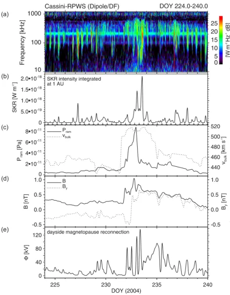
The period DOY 224−240, 2004 was selected because it is centered around two clear peaks in the SKR intensity pro-file occurring on DOY 233.0 and DOY 233.5 as can be seen in Fig. 3b. The intensity profile was established by integrat-ing SKR intensities present in the RPWS dynamic spectrum (shown in Fig. 3a), averaging the profile to a time resolution of 20 min and normalizing intensities to a distance of 1 AU to Saturn. Rapid fluctuations are removed from the profiles by applying a low-pass cos2-filter with a length of 5 h in time domain. The time period displayed in the previous Fig. 2 was selected such that this region of intensified SKR emission is provided.
In Fig. 3b many small ⊥-symbols plotted directly below the SKR intensity profile indicate minima which are caused
by the rotation of Saturn. Neighboring ⊥-symbols are sep-arated by 10.75 h, i.e. the present radio rotation period for Saturn according to Gurnett et al. (2005). In Fig. 3c profiles for the solar wind ram pressure Pram(solid line) and the
so-lar wind bulk velocity vbulk (dotted line) are displayed. In
Fig. 3d the profiles for the magnetic field strength B (solid line) and the y-component By (dotted line) of the IMF in
KSM-coordinates are shown. KSM denotes “Kronocentric Solar Magnetospheric” and is similar to the GSM system used for Earth. The X-axis points from Saturn to the sun, i.e. it is aligned with the local time 12:00 direction. The Y-axis is perpendicular to the plane stretched by the X-axis and the rotation axis of Saturn (Y =×X). The Z-axis completes the right-handed coordinate system. Saturn’s ro-tation axis and magnetic dipole axis differ by <1◦, so the KSM coordinate system can also be related to Saturn’s mag-netic field. Finally, Fig. 3e presents the profile of the dayside magnetopause reconnection voltage 8. For the sake of clar-ity additional profiles for the other input signals listed above in Sect. 3 are not included.
A strong increase of both the bulk velocity (around DOY 231.5) and the ram pressure (peak at DOY 232.9) indicates the arrival of an interplanetary shock at Saturn. Shocks are generated by high-speed plasma flows escaping from coronal holes and overtaking slower moving solar wind plasma. The resulting compression of plasma is followed by several days of rarefaction during which the solar wind speed continuously falls. If such a characteristic pattern of the interplanetary medium is repeated for several successive rotations of the sun, it is called “corotating interaction re-gion” (CIR) (Tsurutani et al., 1982; Gosling, 1996). Since the interplanetary magnetic field is frozen into the plasma
B is also enhanced in a compression region. The profile
for the By-component reveals that the CIR includes a
he-liospheric current sheet (HCS)-crossing around DOY 232.5 when By changes its sign from negative to positive. This
corresponds to a change in the orientation of the tangential component of the IMF from a towards-configuration to an
away-configuration with regard to the position of the sun.
The reconnection voltage generally undulates below 100 kV with a peak of 138 kV. During the period DOY 224−233, i.e. a few days before the strong intensification of SKR, low val-ues for 8 of a few tens of kV are due to low valval-ues of BT and
a mainly southward oriented IMF (θ >90◦). The rate of open flux production accumulated during these 9 days is about 11 GWb (Gigaweber) which is less than the typical amount of open flux in Saturn’s tail (∼35 GWb) deduced from HST aurora observations (Jackman et al., 2004).
In the following, the efficiency functions for the various input signals, i.e. the efficiency as a function of the temporal shift between input and output, will be presented as the key result of the LPT computations (see Eq. 2). The efficiency re-veals the characteristics of the linear filter found by the LPT algorithm.
Fig. 3. (a) The RPWS dynamic spectrum, (b) the integrated SKR intensity profile, (c) profiles for the SW ram pressure (solid) and bulk
velocity (dotted), (d) profiles for the interplanetary magnetic field strength (solid) and its y-component (dotted) in KSM-coordinates and (e) the profile of the reconnection voltage at the dayside magnetopause of Saturn during DOY 224–240, 2004.
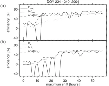
First, it was found that using the time derivative of an input quantity or the absolute value of the input’s time derivative yields a smoother efficiency function than using the original input. For illustration, Fig. 4 displays the efficiency func-tions for the ram pressure and By in combination with the
integrated SKR intensity as output signal, respectively. If the time derivative of the input is used, the input is flagged with an additional δ-symbol. An efficiency function for the abso-lute time derivative of the input is flagged with abs(δ ).
The solid line in Fig. 4a belongs to the efficiency of the ram pressure without performing any derivative. Strong fluc-tuations at small lag times including also negative values are obvious. Negative values indicate that the prediction of SKR intensity by the ram pressure is wrong for these small lag
times. Between 12−13 h lag time the efficiency function ex-hibits a significant increase. This implies that at this temporal shift the influence of variations from the input on variations of the output is a maximum and that this temporal shift may be interpreted as the temporal lag required for the input to trigger the output. Furthermore, the efficiency function levels off at a constant plateau level after 14 h lag time. This means that introducing larger shifts between input and output does not raise the efficiency anymore, so, the filtering between in-put and outin-put is completed after a lag time of 14 h. Figure 4a also includes efficiency functions for the time derivative (dot-ted line) and the absolute value of the time derivative (dashed line) of the ram pressure. One recognizes that the efficiency function for δPram increases smoothly until the maximum
Fig. 4. Efficiency functions for (a) the ram pressure Pramand (b) the By-component of the IMF in combination with SKR intensity as output signal for the time period DOY 224–240, 2004. The re-spective time derivatives of the inputs are flagged with δ and the absolute time derivatives are flagged with abs(δ).
temporal shift of 57.6 h is reached. No significant increase and no constant plateau level is visible indicating a bad lin-ear prediction. For abs(δPram) the situation is different. The
corresponding efficiency function shows a steep increase be-tween 10−12 h lag time, i.e. ∼2 h earlier than for the normal input. Fluctuations in the efficiency function of abs(δPram)
are weaker than in Prammaking a characteristic lag time
eas-ier to identify.
In Fig. 4b the efficiency functions for By and its
deriva-tives are displayed. Again, abs(δBy) (dashed line) reveals a
smoother efficiency function than By (solid line) and a
con-stant plateau level is achieved at ∼26 h lag time. The effi-ciency function for δBy (dotted line) also suggests a
com-pleted filter after 26 h. The efficiency function for the normal input quantity Bystarts to level off about 2 h later, i.e. after
∼28 h.
So, as demonstrated with Pram and By in Fig. 4, a better
efficiency function is obtained by taking the time derivative or the absolute value of the time derivative of the respective input quantity. A good linear prediction is expressed by an efficiency function exhibiting a steep increase at a certain lag time and a subsequent constant plateau level. The higher the plateau level, the better the linear prediction. Plateau levels below 30% are classified as insignificant predictions.
Such insignificant or not well-defined predictions are ob-tained for the following input parameters: the solar wind pro-ton temperature, the magnetic components Bx and Bz, the
modified Akasofu-parameter, the reconnection voltage and the Kelvin-Helmholtz instability quantity. The correspond-ing efficiency functions are displayed in Figs. 5a and 5b.
Fig. 5. In (a) the efficiency functions for the magnetic
compo-nents Bxand Bzand the efficiency function for the time derivative of the SW proton temperature δTp are displayed. Part (b) shows the efficiency functions for the Akasofu-parameter ε, the modified Akasofu-parameter εmod, the reconnection voltage 8 and the KH-instability quantity Q.
The efficiency functions for Bx (solid line) and Bz
(dot-ted line) are settled at low levels and exhibit no significant increase. Taking the time derivatives or absolute time deriva-tives does not improve the result. For the proton tempera-ture the time derivative δTpsmoothes strong fluctuations in
the efficiency function if compared to the original Tp, but
a constant plateau level is not achieved (see dashed line in Fig. 5a). This does not exclude the possibility that a sig-nificant influence of Tp on SKR may be found at larger lag
times beyond 57.6 h. The efficiency function for the KH-instability quantity Q (dashed-dotted line in Fig. 5b) reveals a poor prediction with efficiencies below 20%. Even taking the time derivative or absolute value of the time derivative of
Q does not improve the result. In comparison to the modified
Akasofu-parameter εmod (dotted line), the normal
Akasofu-parameter ε (solid line) yields better results exhibiting a clear plateau level of 47% after ∼45 h lag time. The efficiency function for the reconnection voltage 8 (dashed line) shows a similar behavior as the efficiency function of εmod because
both quantities are dominated by variations of BT and the
polar angle θ .
Another characteristic found was that if the bulk velocity and the magnetic field are mixed, e.g. in B2v, B v2or Bzv2,
then v seems to be of minor influence. Consequently, the efficiencies of B2v, B v2and Bzv2are nearly the same as
for B or Bz alone. The same is true if v is mixed with the
density ρ. As mentioned at the end of Sect. 3, the profiles for ρ v, ρ v2and ρ v3look very similar thus yielding similar efficiency functions.
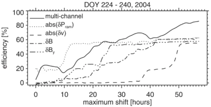
Fig. 6. The efficiency as a function of the temporal shift for the ram
pressure Pram(dotted), the bulk velocity v (dashed), the magnetic field strength B (dash-dot) and the magnetic component By (dash-dot-dot-dot). The time derivative is indicated by δ, the absolute value of the time derivative is indicated by abs(δ ). The solid line is produced if all 4 input signals are mixed in a multi-channel filter.
Finally, four characteristic input signals are left yielding the best results as far as the linear prediction of SKR is con-cerned. These four input quantities are the ram pressure
Pram, the bulk velocity v, the magnetic field strength B and
the y-component Byof the IMF given in KSM-coordinates.
The respective efficiency functions for the time derivative or the absolute value of the time derivative are summarized in Fig. 6. Moreover, Fig. 6 includes the efficiency if all four input signals are processed together in a multi-channel filter (solid line).
It can clearly be seen that the efficiency functions for the absolute time derivative of Pram and v and for the time
derivative of Byexhibit a significant increase in efficiency at
certain temporal shifts. Together with δB all four efficiency functions level off at a constant plateau level. The charac-teristic lag times are ∼(12+1) h for Pram, ∼(51+1) h for v,
∼(43+1) h for B and ∼(26+1) h for By. The additional lag
time (+1) h indicates that a characteristic solar wind struc-ture arrives about 1 h earlier at the dayside magnetopause than at Cassini. This is due to the position of Cassini on its orbit around Saturn and causes an additional acausal shift for the LPT computations which has to be removed. The posi-tion of the dayside magnetopause of Saturn was calculated on the basis of ram pressure data in combination with the mag-netopause model of Slavin et al. (1985). During the time pe-riod DOY 224−240, 2004 Cassini was positioned mainly on the morning side around 06:00 LT. So, e.g. for the ram pres-sure, it can be concluded that the physical processes involved to transform an increase in ram pressure into an increase in SKR intensity require about 13 h as observed by the Cassini spacecraft.
As mentioned before, the efficiency functions for all four input quantities achieve a plateau level at 55%−60% effi-ciency, so, all four input quantities seem to trigger SKR to the same degree of probability.
Fig. 7. Efficiency functions for the absolute time derivative of
the ram pressure abs(δPram) using six different output signals: total SKR intensity integrated over the whole frequency range (solid line), mean intensity (dotted), intensity integrated from 300−1200 kHz (short dashes), frequency bandwidth (dash-dot), up-per SKR frequency limit (dash-dot-dot-dot) and lower SKR fre-quency limit (long dashes).
The solid line in Fig. 6 represents the efficiency function if all 4 inputs are mixed in a multi-channel filter. As can be seen, the efficiency function climbs up to very high values above 80% but it does not level off at a constant plateau. So, investigating the external control of SKR in the frame of a multi-channel filter does not seem to improve the result.
So far, the input signals have been transformed into their respective derivatives to enhance the quality of the linear pre-diction. SKR intensity integrated over the whole frequency range was used as output signal. The following five manip-ulations of the output signal have been tested to check if the results for the efficiency functions can be further enhanced by
- using a mean SKR intensity instead of the integrated total intensity across the whole frequency range - skipping the lower frequency range by integrating
inten-sities just from 300−1200 kHz
- using the SKR frequency bandwidth 1f as output - using the SKR maximum frequency fmaxas output
- using the SKR minimum frequency fminas output.
The resulting efficiency functions for these five manipu-lations using abs(δPram) as input signal are displayed in
Fig. 7. If compared to the total SKR intensity taken as in-put signal (solid line) an integration of intensities just from 300−1200 kHz (short dashes) raises the efficiency function about 10% but fluctuations are a little bit stronger and the in-crease in efficiency around 11 h lag time is less distinct. Tak-ing a mean intensity as output signal lowers the efficiency level significantly (dotted line). If the SKR frequency band-width (dash-dot) is used for output nearly the same result is obtained as taking the upper frequency limit (dash-dot-dot-dot). The lower frequency limit shows the worst results with efficiencies < 20% (long dashes).
These modifications of the output signal have also been ex-ecuted using v, B and Byas inputs. The respective
transfor-mations of the efficiency functions for the different outputs show the same behavior as for the ram pressure displayed in Fig. 7. Another test performed was using the time derivative or absolute value of the time derivative not only for the in-puts but also for the output. No improvements for the linear filter are obtained if these derivatives are applied to the SKR intensity profile both in combination with plasma quantities and magnetic field quantities.
5 Summary and discussion
The Linear Prediction Theory has been applied to Cassini data to investigate the external control of SKR by the solar wind. The results can be summarized as follows:
- Taking the time derivative of an input quantity or the absolute value of its time derivative enhances the effi-ciency function significantly. Characteristic lag times become more distinct and fluctuations of plateau levels are suppressed enabling a better interpretation. It seems that variations of a solar wind input are more important than magnitude values for predicting the SKR intensity profile.
- Four basic input signals (Pram, v, B and By) have been
found to trigger SKR with nearly the same efficiency but at completely different lag times. These lag times and efficiency levels are: Pram→ (∼13 h, 55%), v→
(∼52 h, 55%), B→ (∼44 h, 60%) and By→ (∼27 h,
53%). For the two quantities B and By it may be said
that the efficiency functions are more distinct if a stable sector structure for the IMF is present for several days, i.e. if the interplanetary magnetic field is structured in a CIR pattern. If the shapes of all four efficiency functions are compared to each other, one realizes that the ram pressure exerts the most significant influence on SKR at a certain lag time. Since Pram is interrelated with v, B
and By in a CIR compression region it is not
surpris-ing that also the latter yield similar results for the LPT computations. The important role of the ram pressure for the enhancement of SKR activity will be discussed below on the basis of a model proposed by Cowley et al. (2005).
- Mixing of Pram, v, B and By in the frame of a
multi-channel filter does not enhance the result since in-cluded variations and lag times are too different to com-plement each other. The efficiency function for the multi-channel computations achieves very high values (∼ 85%) but it does not level off at a constant plateau level before the maximum temporal shift of 57.6 h is reached.
- The components Bx and Bzof the IMF are poor
quan-tities for explaining the external control of SKR. The
efficiency functions are either low (≤25%) or the filter-ing does not seem to be completed until the maximum lag time is reached. This does not exclude the possibil-ity that a significant influence of Bxor Bzon SKR may
be found at greater lag times beyond 57 h.
- The Akasofu-parameter yields a quite good linear pre-diction (∼46 h lag time, 47% efficiency) which is, however, less significant than results found for the ram pressure. The modified Akasofu-parameter and the reconnection voltage exhibit much poorer corre-lations with the SKR intensity profile. It seems that the event of prominent SKR intensification occurring around DOY 233, 2004 is not a result of enhanced sub-storm activity initiated by an increased production of open flux in the frame of dayside magnetopause recon-nection. As mentioned above, the predominantly ori-entation of the IMF is from north to south during sev-eral days before DOY 233 thus providing unfavorable conditions for dayside magnetopause reconnection. The maximum of the IMF magnetic field strength does not exceed 1.1 nT.
- The proton temperature and the instability quantity for the Kelvin-Helmholtz instability also yield poor results as far as the linear prediction of SKR is concerned. In the following a short comment on the profile of the KH-instability quantity Q is given. One discrete value of the Q-profile was obtained by searching for the maximum of Q along the dayside magnetopause at a discrete time. So, the obtained profile is actually a Qmax-profile assuming that the position of Qmax at
the dayside magnetopause can be magnetically linked to the true SKR source region near Saturn. If the mag-netic field lines which are penetrating the SKR source region refer to another magnetopause position different from the Qmax-position then another Q must be
consid-ered for the profile. A more detailed study on the basis of Direction-Finding for deriving the correct longitude of the source position would be required resulting in a different profile for Q. Therefore, Cassini must be posi-tioned sufficiently close to the planet because Direction-Finding has an inaccuracy for the SKR source position in the order of 1◦−2◦(Cecconi and Zarka, 2005a). So, taking the Qmax-quantity directly as input for the linear
prediction studies seems to be an insufficient approach in this respect.
- For the output, an intensity profile integrated over fre-quency seems to be the best choice. As modified output signals a mean intensity, the upper frequency limit of SKR, the lower frequency limit and the frequency band-width have also been tested. These modifications for the output yield lower efficiencies. Especially for the outputs concerning the frequency limits, characteristic lag times are shifted to higher values. Furthermore, it was found that the efficiency function for the integrated
intensity profile can be raised further if the integration is just performed from 300−1200 kHz thereby skipping intensity fluctuations which are caused by variations of the lower frequency limit. Thus, these variations seem to be rather due to an internal process, e.g. the rotation of the planet in combination with the specific beam-ing of SKR, than to an external influence from the so-lar wind. So, the integrated SKR intensity profile must be handled with care because it represents SKR activ-ity which was beamed towards a distant observer, i.e. Cassini, located at a specific position around Saturn. This measured profile can by no means represent SKR activity for all possible source regions which are stim-ulated by the solar wind. Furthermore, slight changes in the longitude or latitude of the source region to-gether with the hollow-cone-shaped beaming structure can cause huge intensity variations seen by a quasi-fixed distant observer (Cecconi and Zarka, 2005b).
According to the model of Cowley et al. (2005) intensified auroral and SKR emissions are caused by a compression of Saturn’s magnetosphere as a response to an increased solar wind ram pressure in a CIR compression region. A compres-sion of Saturn’s magnetosphere causes reconnection in open tail lobes due to an enhancement of current densities in the nightside plasma sheet and associated instability configura-tions. As a consequence, a substantial fraction of preexisting open flux is closed (∼20 GWb) during several hours leading to injection of hot plasma into the outer magnetosphere of the nightside polar cap. Newly closed flux tubes are then subcorotated with 50%−80% of rigid corotation from the midnight sector over the dawn sector towards noon due to ionospheric torque. This picture coincides well with HST observations of Saturn’s auroral structures. About 10 h after the onset of the magnetospheric compression bright auroras in the dawn sector have been observed (Clarke et al., 2005). Moreover, hot plasma flows in connection with a substan-tial enhancement of auroral emissions have been detected by Mitchell et al. (2005) and Bunce et al. (2005). The ∼13 h lag time found for the ram pressure thus includes the time required to close a substantial amount of open flux after the onset of magnetospheric compression and to subcorotate an activated SKR source region to the dawn or noon sector from where the radiation is beamed towards the Cassini spacecraft.
Appendix A
Derivation of the filter coefficients for a single-channel filter
First, the used time series (input Xt and measured output
Zt) must be centered around their respective means and they
must be normalized to standard deviation units to ensure that variations and amplitude values of different time series be-come directly comparable. Centered and normalized time
series are indicated by a ∼-sign, e.g. ˜Xt, in order to
distin-guish them from the original data. The error between the measured output ˜Zt and the calculated output ˜Yt is simply
defined as et = ˜Zt− ˜Yt = ˜Zt− M−1 X s=−m fsX˜t −s. (A1) ˜
Yt is replaced by the filtered input signal as outlined in
Eq. (1). The mean-square-error, i.e. the error power I , has to be minimized. If a time series consists of N discrete val-ues then I is given as
I = 1 N − 1 N −1 X t =0 et2 (A2) = 1 N − 1 N −1 X t =0 " ˜ Zt − M−1 X s=−m fsX˜t −s #2 → minimize . (A3)
Minimizing means that the derivation of I after the filter co-efficients fs must be set equal to zero. A total of (M+m)
filter coefficients results in (M+m) derivations and hence in a system of (M+m) normal equations according to
1 N − 1 N −1 X t =0 ˜ ZtX˜t −v− M−1 X s=−m fs 1 N − 1 N −1 X t =0 ˜ Xt −sX˜t −v= 0 (A4) with v = −m, . . . , M − 1
The index v indicates the index s for which the derivation is currently performed. One recognizes that the first sum over t is the definition of the cross-correlation coefficient between
Zt and Xt for a certain temporal shift v. All (M+m)
cross-correlation coefficients as a function of the temporal shift pa-rameter v can be summarized in a vector named Gv.
Simi-larly, the second sum over t in Eq. (A4) represents a vector
Rvstoring all (M+m) auto-correlation coefficients of Xtfor
a constant s. If the sum over s is incorporated, the second term on the left side of Eq. (A4) can be written in matrix notation as M−1 X s=−m fs 1 N − 1 N −1 X t =0 ˜ Xt −sX˜t −v= = M−1 X s=−m fsRv,s= Rvsfs. (A5)
Rvs becomes a square matrix storing all auto-correlation
coefficients of Xt as a function of the shift parameters v
(v= −m, . . . , M−1; row index) and s (s= −m, . . . , M−1; column index). Rvs fulfills the characteristics of a Toeplitz
matrix (Press et al., 1986) which simplifies its computation. So, Eq. (A4) can be written in matrix notation as
The solution of this matrix equation yields a vector storing the filter coefficients according to
fs = (Rvs)−1Gv. (A7)
The computation of the filter coefficients can be summa-rized as follows:
– calculate the cross-correlation coefficients between the measured input Xt and the measured output Zt as a
function of the temporal shift and arrange these coef-ficients in a vector Gv
– calculate the auto-correlation coefficients for the input
Xt as a function of the temporal shift and arrange these
coefficients in a matrix Rvs(Toeplitz matrix)
– insert Gvand Rvsinto Eq. (A7) and compute the filter
coefficients fs.
Acknowledgements. Topical Editor I. A. Daglis thanks P. Galopeau
and another referee for their help in evaluating this paper.
References
Akasofu, S.–I.: Interplanetary energy flux associated with magne-tospheric substorms, Planet. Space Sci., 27, 425–431, 1978. Bunce, E. J., Cowley, S. W. H., Wright, D. M., Coates, A. J.,
Dougherty, M. K., Krupp, N., Kurth, W. S., and Rymer, A. M.: In situ observations of a solar wind compression-induced hot plasma injection in Saturn’s tail, Geophys. Res. Lett., 32, L20S04, 2005.
Cecconi, B., and Zarka, P.: Direction finding and antenna cali-bration through analytical inversion of radio measurements per-formed using a system of two or three electric dipole antennas on a three–axis stabilized spacecraft, Radio Sci., 40, RS3003, doi:10.1029/2004RS003070, 2005a.
Cecconi, B. and Zarka, P.: Model of a variable radio period for Saturn, J. Geophys. Res., 110, A12203, 2005b.
Clarke, J. T., G´erard, J.–C., Grodent, D., Wannawichian, S., Gustin, J., Connerney, J., Crary, F., Dougherty, M., Kurth, W., Cowley, S. W. H., Bunce, E. J., Hill, T., and Kim, J.: Morphological dif-ferences between Saturn’s ultraviolet aurorae and those of Earth and Jupiter, Nature, 433, 717–719, 2005.
Cowley, S. W. H., Badman, S. V., Bunce, E. J., Clarke, J. T., G´erard, J.–C., Grodent, D., Jackman, C. M., Milan, S. E., and Yeoman, T. K.: Reconnection in a rotation-dominated magnetosphere and its relation to Saturn’s auroral dynamics, J. Geophys. Res., 110, A02201, 2005.
Crary, F. J., Clarke, J. T., Dougherty, M. K., Hanlon, P. G., Hansen, K. C., Steinberg, J. T., Barraclough, B. L., Coates, A. J., G´erard, J.–C., Grodent, D., Kurth, W. S., Mitchell, D. G., Rymer, A. M., and Young, D. T.: Solar wind dynamic pressure and elec-tric field as the main factors controlling Saturn’s aurorae, Nature, 433, 720–722, 2005.
Desch, M. D.: Evidence for solar wind control of Saturn radio emis-sion, J. Geophys. Res., 87, 4549–4554, 1982.
Desch, M. D.: Radio emission signature of Saturn immersions in Jupiter’s magnetic tail, J. Geophys. Res., 88, 6904–6910, 1983.
Desch, M. D. and Rucker, H. O.: The relationship between Saturn kilometric radiation and the solar wind, J. Geophys. Res., 88, 8999–9006, 1983.
Desch, M. D. and Rucker, H. O.: Saturn radio emission and the solar wind: Voyager-2 studies, Adv. Space Res., 5, 333–336, 1985. Dougherty, M. K., Kellock, S., Southwood, D. J., Balogh, A.,
Smith, E. J., Tsurutani, B. T., Gerlach, B., Glassmeier, K.–H., Gleim, F., Russell, C. T., Erdos, G., Neubauer, F. M., and Cow-ley, S. W. H.: The Cassini magnetic field investigation, Space Sci. Rev., 114, 331–383, 2004.
Farrell, W. M., Desch, M. D., Kaiser, M. L., Lecacheux, A., Kurth, W. S., Gurnett, D. A., Cecconi, B., and Zarka, P.: A nightside source of Saturn’s kilometric radiation: Evidence for an inner magnetosphere energy driver, Geophys. Res. Lett., 32, L18107, 2005.
Gallagher, D. L., and D’Angelo, N.: Correlations between solar wind parameters and auroral kilometric radiation intensity, Geo-phys. Res. Lett., 8, 1087–1089, 1981.
Galopeau, P. H. M., Zarka, P., and Le Qu´eau, D.: Source location of Saturn’s kilometric radiation: The Kelvin–Helmholtz instability hypothesis, J. Geophys. Res., 100, 26 397–26 410, 1995. Gosling, J. T.: Corotating and transient solar wind flows in three
dimensions, Annu. Rev. Astron. Astrophys., 34, 35–74, 1996. Gurnett, D. A., Kurth, W. S., Kirchner, D. L., Hospodarsky, G. B.,
Averkamp, T. F., Zarka, P., Lecacheux, A., Manning, R., Roux, A., Canu, P., Cornilleau–Wehrlin, N., Galopeau, P., Meyer, A., Bostr¨om, R., Gustafsson, G., Wahlund, J.-E., ˚Ahlen, L., Rucker, H. O., Ladreiter, H. P., Macher, W., Woolliscroft, L. J. C., Al-leyne, H., Kaiser, M. L., Desch, M. D., Farrell, W. M., Harvey, C. C., Louarn, P., Kellogg, P. J., Goetz, K., and Pedersen, A.: The Cassini radio and plasma wave investigation, Space Sci. Rev., 114, 395–463, 2004.
Gurnett, D. A., Kurth, W. S., Hospodarsky, G. B., Persoon, A. M., Averkamp, T. F., Cecconi, B., Lecacheux, A., Zarka, P., Canu, P., Cornilleau-Wehrlin, N., Galopeau, P., Roux, A., Har-vey, C., Louarn, P., Bostrom, R., Gustafsson, G., Wahlund, J.-E., Desch, M. D., Farrell, W. M., Kaiser, M. L., Goetz, K., Kel-logg, P. J., Fischer, G., Ladreiter, H.-P., Rucker, H., Alleyne, H., and Pedersen, A.: Radio and plasma wave observations at Sat-urn from Cassini’s approach and first orbit, Science, 307, 1255– 1259, 2005.
Jackman, C. M., Achilleos, N., Bunce, E. J., Cowley, S. W. H., Dougherty, M. K., Jones, G. H., Milan, S. E., and Smith, E. J.: Interplanetary magnetic field at ∼9 AU during the declining phase of the solar cycle and its implications for Saturn’s magne-tospheric dynamics, J. Geophys. Res., 109, A11203, 2004. Kaiser, M. L., Desch, M. D., Warwick, J. W., and Pearce, J. B.:
Voy-ager detection of nonthermal radio emission from Saturn, Sci-ence, 209, 1238–1240, 1980.
Kaiser, M. L., Desch, M. D., Kurth, W. S., Lecacheux, A., Genova, F., Pedersen, B. M., and Evans, D. R.: Saturn as a radio source, in: Saturn, edited by: Gehrels, T. and Matthews, M. S., Univ. of Arizona Press, Tucson, 378–415, 1984.
Kurth, W. S., Gurnett, D. A., Clarke, J. T., Zarka, P., Desch, M. D., Kaiser, M. L., Cecconi, B., Lecacheux, A., Farrell, W. M., Galopeau, P., G´erard, J.–C., Grodent, D., Prang´e, R., Dougherty, M. K., and Crary, F. J.: An Earth-like correspondence between Saturn’s auroral features and radio emission, Nature, 433, 722– 725, 2005a.
Kurth, W. S., Hospodarsky, G. B., Gurnett, D. A., Cecconi, B., Louarn, P., Lecacheux, A., Zarka, P., Rucker, H. O., Boudjada, M., and Kaiser, M. L.: High spectral and temporal resolution observations of Saturn kilometric radiation, Geophys. Res. Lett., 32, L20S07, 2005b.
Lecacheux, A., Galopeau, P., and Aubier, M.: Re–visiting Satur-nian kilometric radiation with Ulysses/URAP, in: Planetary Ra-dio Emissions IV, edited by Rucker, H. O., Bauer, S. J. and Lecacheux, A., Austrian Academy of Sciences Press, Vienna, 313–325, 1997.
Levinson, N.: The Wiener RMS (root-mean-square) error criterion in filter design and prediction, Appendix B, in: Extrapolation, interpolation, and smoothing of stationary time series with engi-neering applications, edited by: Wiener, N., 1949.
Mitchell, D. G., Brandt, P. C., Roelof, E. C., Dandouras, J., Krim-igis, S. M., Mauk, B. H., Paranicas, C. P., Krupp, N., Hamil-ton, D. C., Kurth, W. S., Zarka, P., Dougherty, M. K., Bunce, E. J., and Shemansky, D. E.: Energetic ion acceleration in Sat-urn’s magnetotail: substorms at Saturn?, Geophys. Res. Lett., 32, L20S01, 2005.
Press, W. H., Flannery, B. P., Teukolsky, S. A., and Vetterling, W. T.: Numerical Recipes, The art of scientific computing, Cambridge University Press, 1986.
Sch¨onwiese, C.–D.: Praktische Statistik f¨ur Meteorologen und Geo-wissenschafter, Geb. Borntr¨ager, Berlin–Stuttgart, 1985. Slavin, J. A., Smith, E. J., Spreiter, J. R., and Stahara, S. S.: Solar
wind flow about the outer planets: gas dynamic modeling of the Jupiter and Saturn bow shocks, J. Geophys. Res., 90, 6275–6286, 1985.
Taubenheim, J.: Statistische Auswertung geophysikalischer und meteorologischer Daten, Verlagges. Geest & Porting, Leipzig, 1969.
Trauger, J. T., Griffiths, R. E., Hester, J. J., Hoessel, J. G., Holtz-man, J. A., Krist, J. E., Mould, J. R., Sahai, R., Scowen, P. A., Stapelfeldt, K. R., and Watson, A. M.: Saturn’s hydrogen aurora: wide-field planetary camera 2 imaging from the Hubble Space Telescope, J. Geophys. Res., 103, 20 237–20 244, 1998.
Tsurutani, B. T., Smith, E. J., Pyle, K. R., and Simpson, J. A.: En-ergetic protons accelerated at corotating shocks – Pioneer 10 and 11 observations from 1 to 6 AU, J. Geophys. Res., 87, 7389– 7404, 1982.
Vasyliunas, V. M., Kan, J. R., Siscoe, G. L., and Akasofu, S.– I.: Scaling relations governing magnetosphere energy transfer, Planet. Space Sci., 30, 359–365, 1982.
Warwick, J. W., Pearce, J. B., Evans, D. R., Carr, T. D., Schauble, J. J., Alexander, J. K., Kaiser, M. L., Desch, M. D., Pedersen, B. M., Lecacheux, A., Daigne, G., Boischot, A., and Barrow, C. H.: Planetary radio astronomy observations from Voyager 1 near Saturn, Science, 215, 239–243, 1981.
Warwick, J. W., Evans, D. R., Romig, J. H., Alexander, J. K., Desch, M. D., Kaiser, M. L., Aubier, M., Leblanc, Y., Lecacheux, A., and Pedersen, B. M.: Planetary radio astronomy observations from Voyager 2 near Saturn, Science, 215, 582–587, 1982. Wiener, N.: Extrapolation, interpolation, and smoothing of
station-ary time series with engineering applications, Publ. Techn. Press of the M.I.T. and John Wiley & Sons Inc., New York, 1949. Wu, C. S., and Lee, L. C.: A theory of terrestrial kilometric
radia-tion, Astrophys. J., 230, 621–626, 1979.
Young, D. T., Berthelier, J. J., Blanc, M., Burch, J. L., Coates, A. J., Goldstein, R., Grande, M., Hill, T. W., Johnson, R. E., Kelha, V., McComas, D. J., Sittler, E. C., Svenes, K. R., Szeg¨o, K., Tanska-nen, P., Ahola, K., Anderson, D., Bakshi, S., Baragiola, R. A., Barraclough, B. L., Black, R. K., Bolton, S., Booker, T., Bow-man, R., Casey, P., Crary, F. J., Delapp, D., Dirks, G., Eaker, N., Funsten, H., Furman, J. D., Gosling, J. T., Hannula, H., Holm-lund, C., Huomo, H., Illiano, J. M., Jensen, P., Johnson, M. A., Linder, D. R., Luntama, T., Maurice, S., McCabe, K. P., Mur-sula, K., Narheim, B. T., Nordholt, J. E., Preece, A., Rudzki, J., Ruitberg, A., Smith, K., Szalai, S., Thomsen, M. F., Viherkanto, K., Vilppola, J., Vollmer, T., Wahl, T. E., West, M., Ylikorpi, T., and Zinsmeyer, C.: Cassini Plasma Spectrometer Investigation, Space Sci. Rev., 114, 1–112, 2004.