HAL Id: hal-00303133
https://hal.archives-ouvertes.fr/hal-00303133
Submitted on 12 Oct 2007HAL is a multi-disciplinary open access
archive for the deposit and dissemination of sci-entific research documents, whether they are pub-lished or not. The documents may come from teaching and research institutions in France or abroad, or from public or private research centers.
L’archive ouverte pluridisciplinaire HAL, est destinée au dépôt et à la diffusion de documents scientifiques de niveau recherche, publiés ou non, émanant des établissements d’enseignement et de recherche français ou étrangers, des laboratoires publics ou privés.
Long-term tropospheric formaldehyde concentrations
deduced from ground-based fourier transform solar
infrared measurements
N. B. Jones, K. Riedel, W. Allan, S. Wood, P. I. Palmer, K. Chance, J.
Notholt
To cite this version:
N. B. Jones, K. Riedel, W. Allan, S. Wood, P. I. Palmer, et al.. Long-term tropospheric formaldehyde concentrations deduced from ground-based fourier transform solar infrared measurements. Atmo-spheric Chemistry and Physics Discussions, European Geosciences Union, 2007, 7 (5), pp.14543-14568. �hal-00303133�
ACPD
7, 14543–14568, 2007 Long-term tropospheric formaldehyde concentrations N. B. Jones et al. Title Page Abstract Introduction Conclusions References Tables Figures ◭ ◮ ◭ ◮ Back Close Full Screen / EscPrinter-friendly Version Interactive Discussion Atmos. Chem. Phys. Discuss., 7, 14543–14568, 2007
www.atmos-chem-phys-discuss.net/7/14543/2007/ © Author(s) 2007. This work is licensed
under a Creative Commons License.
Atmospheric Chemistry and Physics Discussions
Long-term tropospheric formaldehyde
concentrations deduced from
ground-based fourier transform solar
infrared measurements
N. B. Jones1, K. Riedel2, W. Allan2, S. Wood2, P. I. Palmer3, K. Chance4, and J. Notholt5
1
Department of Chemistry, University of Wollongong, NSW 2522, Australia
2
National Institute of Water and Atmospheric Research, New Zealand
3
School of GeoSciences, University of Edinburgh, UK
4
Division of Engineering and Applied Sciences, Harvard University, Cambridge, Massachusetts, USA
5
Institute of Environmental Physics University of Bremen, Bremen, Germany
Received: 27 August 2007 – Accepted: 1 October 2007 – Published: 12 October 2007 Correspondence to: N. B. Jones ([email protected])
ACPD
7, 14543–14568, 2007 Long-term tropospheric formaldehyde concentrations N. B. Jones et al. Title Page Abstract Introduction Conclusions References Tables Figures ◭ ◮ ◭ ◮ Back Close Full Screen / EscPrinter-friendly Version Interactive Discussion
Abstract
Long-term total column measurements of formaldehyde (HCHO) covering a 12 year period from 1992 to 2004 are reported from spectra recorded with a high-resolution Fourier Transform Spectrometer (FTS) using the sun as a light source at a South-ern Hemisphere site (Lauder, New Zealand). The ambient HCHO concentrations at
5
this rural location are often at background levels (<250 ppt) typical for remote marine environments. Due to these low values of HCHO, which are often at or below the detection limit of standard techniques, a method of analysis has been developed that successfully produces HCHO columns with sufficient sensitivity throughout the whole season. The HCHO column over Lauder was found to have a strong seasonal cycle
10
(±50%), with a mean column of 4.2×10¹⁵ molecules cm−2, the maximum occurring
in the summer. A simple box model of CH4 oxidation reproduces the seasonal cycle,
but significantly underestimates the maximum HCHO ground concentrations deduced from the column observations, particularly in summer. This implies the existence of a significant source of HCHO that cannot be explained by oxidation of CH4alone. The
15
ground-based FTS column data compares well with collocated HCHO column mea-surements from the Global Ozone Monitoring Experiment (GOME) satellite instrument (r2=0.65, mean bias=10%, n=48).
1 Introduction
A key challenge in environmental science today is the change in atmospheric
composi-20
tion introduced by increasing emissions of pollutants from human activities. Pollutants introduced into the atmosphere are primarily removed by photo-oxidation. The oxida-tion capacity of the atmosphere is therefore an important indicator of the ability of the atmosphere to cleanse itself.
Formaldehyde (HCHO) is one of the most important species for understanding
25
photo-oxidation pathways in the atmosphere. It is produced by the oxidation of methane 14544
ACPD
7, 14543–14568, 2007 Long-term tropospheric formaldehyde concentrations N. B. Jones et al. Title Page Abstract Introduction Conclusions References Tables Figures ◭ ◮ ◭ ◮ Back Close Full Screen / EscPrinter-friendly Version Interactive Discussion (CH4) and other hydrocarbons, emitted into the atmosphere by plants and animals, and
generated by industrial processes as well as incomplete combustion of biomass and fossil fuels. HCHO is closely linked with the atmosphere’s principal oxidant, the hy-droxyl radical (OH). As a result, HCHO has a relatively short atmospheric lifetime of the order of a few hours.
5
Despite its importance, there are considerable discrepancies between measure-ments of HCHO, and model predictions (for example, Fried et al., 2003; Frost et al., 2002; Jaegl ´e et al., 2000; Riedel et al., 2005), High concentrations of HCHO observed in both the Arctic (Sumner and Shepson, 1999) and Antarctic (Riedel et al., 1999, 2005], suggest photochemical HCHO production at the air-snow interface. Production
10
of free radicals and carbon monoxide (CO) from photolysis of HCHO from this newly discovered source is potentially important for the oxidative capacity of the polar tropo-sphere (Sumner and Shepson, 1999). Modelling of observed HCHO degassing from surface snow implies that this source contributes a significant fraction of the HCHO in the atmospheric boundary layer in the spring and summer (Hutterli et al., 2002; Riedel
15
et al., 2005). While this proposed source largely explains the high Arctic surface fluxes, it does not account for very high Antarctic surface fluxes (Riedel et al., 2005).
Fourier Tranform InfraRed spectroscopy (FTIR), a method that has been rarely used for measuring HCHO, has the potential to address many issues relating to atmospheric HCHO concentrations and trends. This technique has the ability to simultaneously
20
determine the concentrations of both HCHO and CO at the ground. Significant spectral datasets already exist in both the Arctic (Notholt et al., 1997a) and Antarctic (Wood et al., 2004) from state of the art high-resolution FTIR spectrometers, and well as a number of long-term datasets dating back many years at several mid-latitude sites (Rinsland et al., 2003).
25
This paper describes the analysis method and compares HCHO columns and mixing ratios with box model calculations and satellite measurements. In sect. 2 details of the ground based Fourier Transform Spectroscopy (gb-FTS) are given including a formal error analysis. Section 3.1 describes the results of the analysis on 12 years of infrared
ACPD
7, 14543–14568, 2007 Long-term tropospheric formaldehyde concentrations N. B. Jones et al. Title Page Abstract Introduction Conclusions References Tables Figures ◭ ◮ ◭ ◮ Back Close Full Screen / EscPrinter-friendly Version Interactive Discussion (IR) data from Lauder, New Zealand; Sect. 3.2 outlines a simple box model based on
CH4oxidation chemistry, while Sect. 3.3 compares the gb-FTS results with co-located
measurements from GOME.
2 Method
The infrared spectra used in this study are from the Network for the Detection of
Atmo-5
spheric Composition Change (NDACC,http://www.ndacc.org/) primary Southern Hemi-sphere station at Lauder (45◦S, 169◦E, 0.37 km a.s.l.). The time period covers 12 years
from 1992 to 2005, and as such, season to season changes can be studied along with long term trends. The instrumentation and Lauder program history is described in more detail in previous papers (Jones et al., 1994; Jones et al., 2001; Rinsland et al., 2002).
10
HCHO is a weak absorber in the mid-infrared with absorption depths of less than 1% under normal background conditions. Its quantification must therefore be done in a careful manner. The chosen lines are all part of the ν1and ν5stretches, with the band centers located at 2782 cm−1 and 2843 cm−1 respectively. The micro-windows that have been adopted for use in the mid-IR in this study are based on 5 windows selected
15
by using the method reported by Notholt et al. (2006). Table 1 outlines the windows, wavelength ranges and interfering species. Because there are several major interfering species in all microwindows, the concentration profiles of the interfering gases CH4and
O3were determined simultaneously with HCHO, while a single scaling parameter was used for other gases. Further, pre-fitting several of these interferring gases (HDO, H2O,
20
N2O, and CH4) in wavenumber regions specifically selected to obtain better estimates
of their individual a priori profiles (labelled as step 1 in Table 1) gave more consistent results; for HDO and H2O this is due to the large variability of atmospheric humidity levels. There are also very small but significant absorptions from solar CO; significant in the context that the absorptions are very similar in shape to the HCHO feature in
25
the 2869.650–2870.100 cm−1window. To overcome this potential source of ambiguity, a relatively isolated solar CO feature was fitted simultaneously in a separate window
ACPD
7, 14543–14568, 2007 Long-term tropospheric formaldehyde concentrations N. B. Jones et al. Title Page Abstract Introduction Conclusions References Tables Figures ◭ ◮ ◭ ◮ Back Close Full Screen / EscPrinter-friendly Version Interactive Discussion (2856.10–2856.35 cm−1) with only very minor interferences from CH4and N2O.
All spectra were recorded using a 700 cm−1wide filter centered at 2750 cm−1. Since the HCHO spectral signature is very weak and broad (as the peak of its density is close to the ground and therefore completely dominated by pressure broadening), the resolution of the spectra were reduced to 0.02 cm−1 (optical path difference of 50 cm)
5
and apodised with a triangular function, thus reducing the high frequency noise, and increasing the signal to noise ratio (SNR) of the spectra to around 2000:1.
The algorithm used in the inversion, SFIT2 (version 3.91), has been developed jointly by several groups within the NDACC (NASA Langley Research Center, University of Denver, NCAR, NIWA Lauder, and the University of Wollongong). SFIT2 is capable
10
of retrieving the vertical profiles of several gases simultaneously from ground-based infrared spectra. The inverse model is based on a semi-empirical application of the op-timal estimation method (OEM) (Rodgers, 2000). Both the forward and inverse models have been described previously (Rinsland et al., 1998). The earlier simple solar model used in SFIT2, however, has been replaced with a more accurate algorithm (Hase et
15
al., 2004).
The global SNR assumed in the retrieval was 1200, and was reduced to slightly lower values in selected spectral intervals (see Table 1) due to consistent residual features in the fitted spectra caused by various inaccuracies in line parameters or unknown absorbers.
20
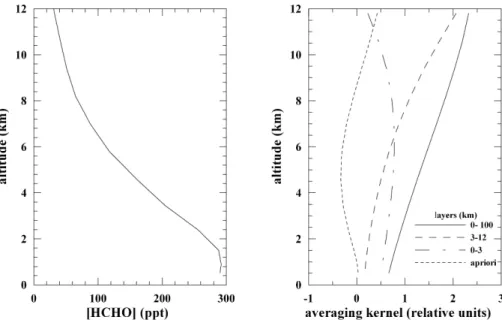
The OEM uses an assumed a priori concentration for all gases. In this study the HCHO a priori profile is based on aircraft profile measurements (NASA/PEM-Tropics B, Singh et al., 2001) and is shown in Fig. 1a. The a priori profile decreases expo-nentially in the troposphere, with a concentration of 290 ppt at the ground. The scale height is approximately 6.2 km in mixing ratio, with a HCHO density scale height of
25
4.2 km. The 1 sigma uncertainties used in the OEM are directly employed in the a pri-ori covariance matrix as a tuning parameter, i.e. they are adjusted empirically to obtain stable retrievals while obtaining the maximum possible spectral information. The spe-cific method used here was to adopt a 1 sigma value at the ground that is consistent
ACPD
7, 14543–14568, 2007 Long-term tropospheric formaldehyde concentrations N. B. Jones et al. Title Page Abstract Introduction Conclusions References Tables Figures ◭ ◮ ◭ ◮ Back Close Full Screen / EscPrinter-friendly Version Interactive Discussion with reported variability in the Pacific region (Fried et al., 2003; Singh et al., 2001) of
125%, exponentially decreasing to 10% at the tropopause. The a priori profile for all other gases are based on a range of measurements from both balloons (e.g. MarkIV In-terferometer, Toon et al., 1999), satellites (e.g. Upper Atmospheric Research Satellite,
http://badc.nerc.ac.uk/data/uars/), and local sondes (for H2O and O3) launched weekly
5
from the Lauder site. Figure 1b shows the averaging kernels for the tropospheric part of the HCHO profile; there is a clear semi-independent kernel from 0–3 km, consistent with the degrees of freedom for signal (DOFS) of 1.2 to 1.8 (the range here reflects the range of solar zenith angles in the measurements).
We present in Sect. 3.3 the first multi-year comparison between the gb-FTS data
10
and space-borne column measurements of HCHO from the GOME satellite instrument, which provides an independent validation dataset.
3 Results and discussion
3.1 Column averaged time-series
The full dataset is shown in Figs. 2 and 3. The HCHO total column is displayed in Fig. 2.
15
The depicted points (diamonds) are monthly means, with error bars that are computed from the root mean square error of all measurements within the month, assuming an error of 16% per measurement (Table 2). This 16% error includes random components from smoothing (10.5%), measurement (13.2%) and temperature (1.2%) errors, and the systematic spectroscopic errors from uncertainties in the line strength (4.6%), air
20
broadening half-width (6.6%), and the effective apodization parameter (0.9%), a mea-sure of the instrumental performance. The error terms for all random error components were computed using the OEM formalism (i.e. by calculating the gain and sensitivity matrices), while the systematic error terms were dealt with using perturbation meth-ods. A selection of spectra (50) were chosen at random with a range of zenith angles
25
and HCHO column amounts, and their columns were compared with the same spectra 14548
ACPD
7, 14543–14568, 2007 Long-term tropospheric formaldehyde concentrations N. B. Jones et al. Title Page Abstract Introduction Conclusions References Tables Figures ◭ ◮ ◭ ◮ Back Close Full Screen / EscPrinter-friendly Version Interactive Discussion analysed with the systematic error component terms perturbed by either 10% (the line
strength and the effective apodization parameter were multiplied by a factor of 1.1) or 5% (the air broadened half width was decreased by 5%). All errors are listed in Table 2. Also plotted in Fig. 2 (solid line) is the following function that consists of seasonal and trend terms:
5
HCHO(t) = a0+ a1t + a2t2+ a3cos[(2π(t − φ1)] + a4cos[π(t − φ2)] (1)
where HCHO(t) is the HCHO column at time t, a0the mean HCHO column at the start of the fitting interval (1992.2), a1 the linear change in column, a2a quadratic term, a3
and a4the amplitudes of annual and semi-annual seasonal modulations respectively,
and φ1and φ2the annual and semi-annual phases respectively. The fitted coefficients
10
for the total column are given in Table 3. The data show a clear seasonal cycle with a summer maximum and winter minimum, consistent with expected photochemical control by OH and known NOx sources at the site (see Sect. 3.2). While there are statistically insignificant trends and semi-annual effects, there are obvious departures from the mean seasonal trends in the summers of 1999, 2000, and 2002.
15
Similarly, Fig. 3 shows partial columns of HCHO over two different height ranges, 0–3 km (red diamonds) and 3–12 km (black diamonds), for the same time period as the HCHO total column data in Fig. 2. These height ranges correspond to the averaging kernel function height ranges discussed in the previous section (see Fig. 1). The solid red (0–3 km) and black (3–12 km) lines are fitted using Eq. (1) with the corresponding
20
coefficients presented in Table 3. The error bars in Fig. 2 above, were computed for both random and systematic terms. They are listed in Table 2. The overall features of these two partial columns are comparable to each other as well as the total column results from Fig.1 as would be expected from retrievals of HCHO with limited vertical resolution. However there are notable features in the data occurring between 1999 and
25
2002, referred to earlier, which appear to be prominent in the 0–3 km partial column but not to the same extent above this. This feature is particularly evident in the summer of 1999 where there is a factor 3 difference between the mean 1999 HCHO column and the peak summer value. In 2000 and 2002 this difference (factor of 2) is less,
ACPD
7, 14543–14568, 2007 Long-term tropospheric formaldehyde concentrations N. B. Jones et al. Title Page Abstract Introduction Conclusions References Tables Figures ◭ ◮ ◭ ◮ Back Close Full Screen / EscPrinter-friendly Version Interactive Discussion while it is not always clear which partial column is perturbed the most with respect to
the mean. In other years, the HCHO column seems to be well captured by the simple seasonal fit, particularly in the last two years of data. Most of this interannual difference corresponds with long-range transport of biomass burning plumes from Australia, with very high values of HCHO, a known biomass burning emission product, associated
5
with particularly severe burning events in New South Wales (Paton-Walsh et al., 2004; Paton-Walsh et al., 2005).
Mahieu et al. (1997) reported a mean HCHO column of 5.9±1.5×10¹⁴ molecules cm−2 above the International Scientific Station of the Jungfraujoch (3.57 km a.s.l.), Switzerland, from a high resolution FTIR averaged over the time period from 1988
10
to 1996. Data binned into several day averages were also reported by Mahieu et al. (1997) but unlike the results presented here, seasonal effects were less clear. The other studies that report multi-year datasets are two papers by Notholt et al. (1997b, 2000) who published column HCHO data from ground based instruments in the Arctic (Ny Alesund, 78.9◦N, 11.9◦E) and the Antarctic (McMurdo, 77.9◦N, 166.7◦E ) covering
15
4 seasons in the case of Ny Alesund and a single campaign in Antarctica (September– October 1986). The Ny Alesund data in particular show seasonal behavior of a magni-tude (range 2–5×10¹⁵ molecules cm−2) and phase consistent with our results, but are also affected by direct transport of pollutants from the European continent in the winter (giving a second maximum).
20
Figure 3 also shows, in the right hand axis, the HCHO concentrations for the two plotted layers. These concentrations are estimated by calculating the ratio of the re-trieved partial column for the layer divided by the total air mass in the respective partial column.
3.2 Box modelling
25
We are currently developing a chemical box model to simulate gas-phase atmospheric chemistry in the boundary layer above Lauder. Here we present preliminary results relating to the generation of HCHO from CH4, and how this compares with the
ACPD
7, 14543–14568, 2007 Long-term tropospheric formaldehyde concentrations N. B. Jones et al. Title Page Abstract Introduction Conclusions References Tables Figures ◭ ◮ ◭ ◮ Back Close Full Screen / EscPrinter-friendly Version Interactive Discussion vations reported above.
Our initial model setup uses the basic gas-phase chemistry of the Master Chemical Mechanism version 3 (MCMv3) e.g., (Saunders et al., 2003). We use the MCMv3 functional forms for the appropriate photolysis j-values, but normalize their mid-day values to the corresponding values obtained from the Tropospheric Ultraviolet Visible
5
(TUV) model (Madronich and Flocke, 1998) at the position of Lauder. Appropriate dry deposition rates are applied for HCHO, CH3OOH, H2O2, O3, etc.
The level of NOx (NO + NO2) has a strong influence on the production of HCHO
from the precursor species CH3O2and CH3O. Measurements of NOxare not routinely
made at Lauder. However, Johnston and Mckenzie (1984) found using long path
spec-10
troscopic absorption that the tropospheric mixing ratio of NO2at Lauder was extremely variable. Values ranged from below the measurement threshold of about 20 ppt during windy conditions, to well over 1 ppb under still conditions, with typical values of a few hundred ppt.
We ran our model under mid-June (winter) and mid-December (summer) conditions
15
for 30 days to ensure the system had reached equilibrium and that the maximum HCHO levels for the conditions were obtained, although generally only a few days were re-quired to reach equilibrium. CH4, O3, and CO were constrained to synoptic values in
all cases. A boundary layer thickness of 1 km was chosen, consistent with the find-ings of Johnston and Mckenzie (1984). Simulations were run for a range of mean NOx
20
values between 20 ppt and 1000 ppt.
We found that for a 24-h mean value of 20 ppt NOx, the 24-h mean HCHO mixing
ratio in June was approx. 50 ppt, and in December approx. 150 ppt. In June, the HCHO reached a maximum mean value of approx. 220 ppt when the mean NOx was about 400 ppt, decreasing slowly for larger NOx values. In December, the HCHO reached a
25
maximum mean value of approx. 480 ppt when the mean NOxwas about 700 ppt, again
decreasing slowly for larger NOxvalues. These maxima in HCHO arise because of the action of NOxin depleting the precursor species CH3O2and CH3O during the formation
of extra HCHO. Although the HCHO values are strongly dependent on the ambient NOx
ACPD
7, 14543–14568, 2007 Long-term tropospheric formaldehyde concentrations N. B. Jones et al. Title Page Abstract Introduction Conclusions References Tables Figures ◭ ◮ ◭ ◮ Back Close Full Screen / EscPrinter-friendly Version Interactive Discussion level, the model results imply a significant seasonal cycle in HCHO should exist, as is
indeed seen in the results presented in Sect. 3.1. Assuming a scale height of 6.2 km (Sect. 3.1), the expected total column of HCHO from CH4 oxidation is approximately
in the range of 1.9 to 4.1×10¹⁵ molecules cm−2for the high NOxassumption of 400 to
700 ppt.
5
The simulations suggest that winter and summer HCHO mixing ratios (derived from CH4alone) of up to 220 ppt and 480 ppt respectively can plausibly be explained by the
existence of NOx mixing ratios of at least 400 ppt and 700 ppt in winter and summer respectively. At present, we do not have concurrent measurements of HCHO and NOx
to confirm this. However, a notable feature of the measurements described in Sect. 3.1
10
is the regular occurrence of HCHO mixing ratios significantly larger than 480 ppt. Our simulations suggest that these high HCHO values cannot be explained by oxidation of CH4alone.
A possible additional HCHO precursor is isoprene (C5H8), the oxidation of which can yield relatively large quantities of HCHO e.g., (Carter and Atkinson, 1996;
Zimmer-15
mann and Poppe, 1996). Lewis et al. (2001) measured isoprene mixing ratios up to 120 ppt at Cape Grim, Tasmania, in air masses originating principally from Tasmanian forest and grassland. It is possible that similar high isoprene episodes can occur at Lauder. Another possibility is that HCHO from biomass burning events, either local or transported from Australian bush fires (see Sect. 3.1), could be contributing to the
20
seasonal large HCHO values measured at Lauder. 3.3 A comparison with GOME HCHO vertical columns
The Global Ozone Monitoring Experiment (GOME) is a space-based grating spectrom-eter that measures backscattered solar radiation in the UV/VIS spectral range (240– 790 nm) at a spectral resolution of 0.2–0.4 nm (Burrows et al., 1999). HCHO slant
25
columns are fitted in the 336–356 nm wavelength region with a mean column fitting un-certainty of 4×10¹⁵ molec cm−2 (Chance et al., 2000). An air-mass factor (AMF) that accounts for scattering processes from aerosols and clouds, in addition to Rayleigh
ACPD
7, 14543–14568, 2007 Long-term tropospheric formaldehyde concentrations N. B. Jones et al. Title Page Abstract Introduction Conclusions References Tables Figures ◭ ◮ ◭ ◮ Back Close Full Screen / EscPrinter-friendly Version Interactive Discussion scattering, is used to convert these slant columns to vertical columns (Palmer et al.,
2001). For the work shown here we use only GOME data with an associated cloud fraction of less than 40% and with the geolocation of the gb-FTS located within the corner coordinates of the 320×40 km2GOME pixel (which occurs on average every 3 days).
5
Figure 4 shows GOME averaging kernels that are derived using the method de-scribed by Eskes and Boersma (2003) based on the Rodgers formulation (Rodgers, 2000) for summer (red) and winter (blue) profiles, while the averaging kernel for the gb-FTS is plotted in green for reference (from Fig. 1). The GOME averaging kernels are the means of assumed summer/winter model profiles from GEOS-Chem (Bey et al.,
10
2001) at several different airmasses. The specific computation assumes that the slant column is linear with respect to gas amount and that the dependence of the spectrum on the HCHO vertical distribution can be described by a single scaling factor (Eskes and Boersma, 2003). The averaging kernel for each layer can therefore be expressed as the ratio of the air-mass factor for the particular layer to the total a priori air-mass
15
factor. While there are clear differences in the relative weights of the GOME and gb-FTS averaging kernels, in the lower half of the troposphere (below about 6 km), the kernels are reasonably similar in magnitude and shape. Both the gb-FTS and GOME averaging kernels tend to over-weight the HCHO column in the upper troposphere but this has little effect on the column due to the rapidly decreasing HCHO mixing ratio.
20
The nature of the analysis techniques, instruments, platforms and geometries mean that the two datasets are not directly comparable. We have therefore used the method outlined by Rodgers and Connor (2003). For simplicity, we assume that the gb-FTS is the “truth”, against which the GOME measurement is compared. We can there-fore write the following expression, following the nomenclature of Rodgers and Connor
25
(2003), that relates the GOME column with the gb-FTS derived column: ˜
CGf = Cc+ aTG( ˜xf − xc) (2)
where ˜CGf is the smoothed gb-FTS column, Ccthe ensemble gb-FTS column average,
ACPD
7, 14543–14568, 2007 Long-term tropospheric formaldehyde concentrations N. B. Jones et al. Title Page Abstract Introduction Conclusions References Tables Figures ◭ ◮ ◭ ◮ Back Close Full Screen / EscPrinter-friendly Version Interactive Discussion
aTG the transpose of the GOME column averaging kernel, ˜xf the gb-FTS mixing ratio
profile, and xcthe gb-FTS ensemble average mixing ratio profile. The gb-FTS
ensem-ble averages for both the column and vertical profile were taken as the mean from all gb-FTS data.
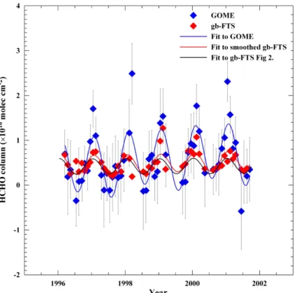
Figure 5 shows the monthly mean smoothed gb-FTS total columns along with GOME
5
total columns over the time period of 1996 to 2001. The GOME data has been averaged with a 21 day running mean and regridded spatially to match all gb-FTS monthly mean data points, a total of 51 data values over the 1996 to 2001 time period. The GOME data was also uniformly scaled down by 20% according to recent laboratory UV cross section measurements of HCHO (Gratien et al., 2007). The use of monthly mean data
10
was adopted for two reasons, 1) to improve the statistics of the presented data due to the inherently very weak spectroscopic lines, and 2) to average over large short-term (order of hours) variability in the HCHO concentration from local sources near the ground that will affect the gb-FTS measurements but will be more than likely missed by GOME (both spatially and temporally). Also shown in Fig. 5 are three fitted curves,
15
using equation 1) to the regridded GOME data (solid blue line), gb-FTS data smoothed with the GOME summer or winter averaging kernel (solid red line), and the original pre-smoothed fit to the gb-FTS data (dotted red line) as displayed in Fig. 2. The smoothing operation on the gb-FTS data had little effect on the ground-based data. The two datasets are in good agreement in terms of seasonal trends (the fitted phases agree
20
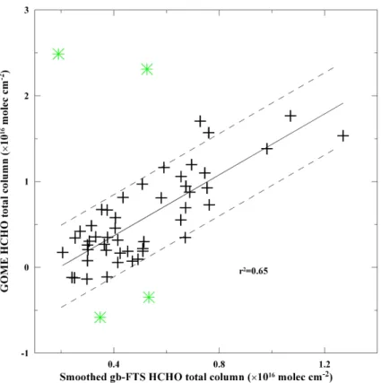
to within their respective errors, see Table 3), but the magnitudes of their respective cycles and year-to-year variations are clearly different. The variance in the GOME columns is much higher than the gb-FTS data. Figure 6 shows a correlation plot of the smoothed gb-FTS data against the regridded GOME data. The correlation coefficient r2 is 0.65, indicating that the two datasets are well correlated, driven mainly by the
25
annual season change. A simple statistical analysis on the means of the total columns of the two datasets using a T-test (gb-FTS=5.1±0.3, GOME = 5.6±0.7, both in units of 1015molecules cm−2), gives a T paired value of 1.2 and an associated P-value of 0.22 for 49 degrees of freedom, i.e., the means are not statistically different. In the test we
ACPD
7, 14543–14568, 2007 Long-term tropospheric formaldehyde concentrations N. B. Jones et al. Title Page Abstract Introduction Conclusions References Tables Figures ◭ ◮ ◭ ◮ Back Close Full Screen / EscPrinter-friendly Version Interactive Discussion excluded three outliers, marked with green stars.
In general the two datasets agree very well given the preliminary nature of this com-parison. On seasonal scales the two HCHO data sets (ground and space based) agree to within their respective errors. However, the GOME data does appear to show larger variations in the columns throughout anyone particular year. This is indicative of
influ-5
ences from heterogeneous sources being captured by one measuring platform, and not the other. We note that the east and west coasts of the South Island of New Zealand have significantly different vegetation types, the west being wet with large tracks of dense forest, while the east coast is dry and less vegetated. The exact orbital path of the spacecraft could therefore have an impact on whether short term volatile
com-10
pounds like HCHO are successfully correlated with ground based observations. How-ever, as the HCHO concentrations are normally at background levels, the agreement between the two data sets is remarkable given the difficulties of the HCHO measure-ments from both the gb-FTS and GOME platform. New data products from the Ozone Monitoring Instrument (OMI) will likely improve this statistical comparison because of
15
better spatial and temporal resolution of the OMI measurement.
4 Summary and conclusions
Long-term total column measurements of HCHO are reported from the Southern Hemi-sphere site at Lauder, New Zealand, and compared with co-located satellite measure-ments and a box model. A robust method of retrieving HCHO columns from ground
20
based remotely sensed infrared spectra is described. As the low ambient HCHO con-centrations often recorded at Lauder are often close to detection level, this poses a challenge for analysis techniques. The mean HCHO column over Lauder from 1992 to 2005 was 4.0±0.3×10¹⁵ molecules cm−2, with a strong seasonal cycle (±50%) maxi-mizing in the summer. A simple box model reproduces the seasonal cycle, but
signif-25
icantly underestimates the maximum HCHO ground concentrations deduced from the column observations, particularly in summer. This cannot be explained by oxidation of
ACPD
7, 14543–14568, 2007 Long-term tropospheric formaldehyde concentrations N. B. Jones et al. Title Page Abstract Introduction Conclusions References Tables Figures ◭ ◮ ◭ ◮ Back Close Full Screen / EscPrinter-friendly Version Interactive Discussion CH4alone and therefore implies the existence of a significant extra source of HCHO. A
comparison of the ground-based FTS column data with collocated measurements from the GOME satellite instrument shows good agreement in the respective mean HCHO columns with the data also being well correlated (r2=0.65).
Acknowledgements. Support of the Australian Research Council is gratefully acknowledged
5
as well as funding from the New Zealand Foundation for Research, Science, and Technology (contract C01X0204) that supports work at NIWA. We also thank I. De Smedt for very helpful discussions on the GOME averaging kernel calculations.
References
Bey, I., Jacob, D. J., Logan, J. A., et al.: Global modeling of tropospheric chemistry with
assimi-10
lated meteorology: Model description and evaluation, J. Geophys. Res., 106, 23 073–23 095, 2001.
Burrows, J. P., Weber, M., Buchwitz, M., et al.: The Global Ozone Monitoring Experiment (GOME): Mission moncept and first scientific results, J. Atmos. Sci., 56(2), 151–175, 1999. Carter, W. P. L. and Atkinson, R.,: Development and evaluation of a detailed mechanism for the
15
atmospheric reactions of isoprene and NOx, Int. J. Chem. Kinet., 28(7), 497–530, 1996. Chance, K., Palmer, P. I., Spurr, R. J. D., et al.: Satellite observations of formaldehyde over
North America from GOME, Geophys. Res. Lett., 27(21), 3461–3464, 2000.
Eskes, H. J. and Boersma, K. F.: Averaging kernels for DOAS total-column satellite retrievals, Atmos. Chem. Phys., 3, 1285–1291, 2003,
20
http://www.atmos-chem-phys.net/3/1285/2003/.
Fried, A., Crawford, J., Olson, J., et al.: Airborne tunable diode laser measurements of formaldehyde during TRACE-P: Distributions and box model comparisons, J. Geophys. Res.-Atmos., 108(D20), 8798, doi:10.1029/2003JD003451, 2003.
Frost, G. J., Fried, A., Lee, Y. N., et al.: Comparisons of box model calculations and
measure-25
ments of formaldehyde from the 1997 North Atlantic Regional Experiment, J. Geophys. Res., 107(D7-8), 4060, doi:10.1029/2001JD000896, 2002.
Gratien, A., Picquet-Varrault, B., Orphal, J., et al.: Laboratory intercomparison of the formalde-hyde absorption cross sections in the infrared (1660–1820 cm−1) and ultraviolet(300–
ACPD
7, 14543–14568, 2007 Long-term tropospheric formaldehyde concentrations N. B. Jones et al. Title Page Abstract Introduction Conclusions References Tables Figures ◭ ◮ ◭ ◮ Back Close Full Screen / EscPrinter-friendly Version Interactive Discussion 360 nm) spectral regions, J. Geophys. Res., 112(D05305), doi:10.1029/2006JD007201,
2007.
Hase, F., Hannigan, J. W., Coffey, M. T., et al.: Intercomparison of retrieval codes used for the analysis of high-resolution, ground-based FTIR measurements, J. Quant. Spectrosc. Radiat. Transf., 87(1), 25–52, 2004.
5
Hutterli, M. A., Bales, R. C., McConnell, J. R., et al.: HCHO in Antarctic snow: Preservation in ice cores and air-snow exchange, Geophys. Res. Lett., 29(8), 1235, doi:10.1029/2001GL014256, 2002.
Jaegl ´e, L., Jacob, D. J., Brune, W. H., et al.: Photochemistry of HOx in the upper troposphere at northern midlatitudes, J. Geophys. Res., 105(D3), 3877–3892, 2000.
10
Johnston, P. V. and McKenzie, R. L.: Long-path absorption measurements of tropospheric NO2 in rural New Zealand, Geophys. Res. Lett., 11(1), 69–72, 1984.
Jones, N. B., Koike, M., Matthews, W. A., et al.: Southern hemisphere seasonal cycle in total column nitric acid, Geophys. Res. Lett., 21(7), 593–596, 1994.
Jones, N. B., Rinsland, C. P., Liley, J. B., et al.: Correlation of aerosol and carbon monoxide at
15
45 S: evidence of biomass burning emissions, Geophys Res Lett, 28(4), 709–712, 2001. Lewis, A. C., Carpenter, L. J., and Pilling, M. J.: Nonmethane hydrocarbons in southern ocean
boundary layer air, J. Geophys. Res.-Atmos., 106(D5), 4987–4994, 2001.
Madronich, S. and Flocke, S. (Eds.): The role of solar radiation in atmospheric chemistry, 1-26 pp., Springer-Verlag, Heidelberg, 1998.
20
Mahieu, E., Zander, R., Delbouille, L., et al.: Observed trends in total vertical column abun-dances of atmospheric gases from IR solar spectra recorded at the Jungfraujoch, J. Atmos. Chem.. , V28(1), 227–243, 1997.
Notholt, J., Toon, G., Jones, N., et al.: Automatic line finding program for atmospheric remote sensing, J. Qant. Spectro. Radia. Trans., 97(1), 112–125, 2006.
25
Notholt, J., Toon, G., Stordal, F., et al.: Seasonal variations of trace gases in the high Arctic at 79◦N, J. Geophys. Res., 102(D11), 12 855–12 861, 1997a.
Notholt, J., Toon, G. C., Lehmann, R., et al.: Comparison of Arctic and Antarctic trace gas column abundances from ground-based Fourier transform infrared spectrometry, J. Geophys. Res., 102(D11), 12 863–12 870, 1997b.
30
Notholt, J., Toon, G. C., Rinsland, C. P., et al.: Latitudinal variations of trace gas concentrations in the free troposphere measured by solar absorption spectroscopy during a ship cruise, J. Geophys. Res., 105(D1), 1337–1350, 2000.
ACPD
7, 14543–14568, 2007 Long-term tropospheric formaldehyde concentrations N. B. Jones et al. Title Page Abstract Introduction Conclusions References Tables Figures ◭ ◮ ◭ ◮ Back Close Full Screen / EscPrinter-friendly Version Interactive Discussion Palmer, P. I., Jacob, D. J., Chance, K., et al.: Air mass factor formulation for spectroscopic
measurements from satellites: Application to formaldehyde retrievals from the Global Ozone Monitoring Experiment J. Geophys. Res., 106(D13), 14 539–14 550, 2001.
Paton-Walsh, C., Jones, N., Wilson, S., et al.: Trace gas emissions from biomass burning inferred from aerosol optical depth, Geophys. Res. Lett., 31(5), L05116,
5
doi:10.1029/2003GL018973, 2004.
Paton-Walsh, C., Jones, N. B., Wilson, S. R., et al.: Measurements of trace gas emissions from Australian forest fires and correlations with coincident measurements of aerosol optical depth, J. Geophys. Res., 110, D24305, doi:10.1029/2005JD006202, 2005.
Riedel, K., Allan, W., Weller, R., et al.: Discrepancies between formaldehyde
measure-10
ments and methane oxidation model predictions in the Antarctic troposphere: An as-sessment of other possible formaldehyde sources, J. Geophys. Res., 110, D15308, doi:10.1029/2005JD005859, 2005.
Riedel, K., Weller, R., and Schrems, O.: Variability of formaldehyde in the Antarctic troposphere, Phys. Chem. Chem. Phys, 1, 5523–3327, 1999.
15
Rinsland, C. P., Jones, N. B., Connor, B. J., et al.: Northern and southern hemisphere ground-based infrared spectroscopic measurements of tropospheric carbon monoxide and ethane, J. Geophys. Res., 103, 28 197–28 218, 1998.
Rinsland, C. P., Jones, N. B., Connor, B. J., et al.: Multiyear infrared solar spectroscopic mea-surements of HCN, CO, C2H6, and C2H2tropospheric columns above Lauder, New Zealand
20
(45◦S latitude), J. Geophys. Res., 107(D14), 4185, doi:10.1029/2001JD001150, 2002.
Rinsland, C. P., Mahieu, E., Zander, R., et al.: Long-term trends of inorganic chlorine from ground-based infrared solar spectra: Past increases and evidence for stabilization, J. Geo-phys. Res., 108(D8), 4252, doi:10.1029/2002JD003001, 2003.
Rodgers, C. D.: Inverse Methods for Atmospheric Sounding, 238 pp., World Scientific, London,
25
2000.
Rodgers, C. D. and Connor, B. J.: Intercomparison of remote sounding instruments, J. Geo-phys. Res., 108(D3), 4116, doi:4110.1029/2002JD002299, 2003.
Saunders, S. M., Jenkin, M. E., Derwent, R. G., et al.: Protocol for the development of the Master Chemical Mechanism, MCM v3 (Part A): tropospheric degradation of non-aromatic
30
volatile organic compounds, Atmos. Chem. Phys., 3, 161–180, 2003, http://www.atmos-chem-phys.net/3/161/2003/.
Singh, H., Chen, Y., Staudt, A., et al.: Evidence from the Pacific troposphere for large global 14558
ACPD
7, 14543–14568, 2007 Long-term tropospheric formaldehyde concentrations N. B. Jones et al. Title Page Abstract Introduction Conclusions References Tables Figures ◭ ◮ ◭ ◮ Back Close Full Screen / EscPrinter-friendly Version Interactive Discussion sources of oxygenated organic compounds, Nature, 410(6832), 1078–1081, 2001.
Sumner, A. L. and Shepson, P. B.: Snowpack production of formaldehyde and its effect on the Arctic troposphere, Nature, 398(6724), 230–233, 1999.
Toon, G. C., Blavier, J. F., Sen, B., et al.: Comparison of MkIV balloon and ER-2 aircraft measurements of atmospheric trace gases, J. Geophys. Res., 104(D21), 26 779–26 790,
5
1999.
Wood, S. W., Batchelor, R. L., Goldman, A., et al.: Ground-based nitric acid measurements at Arrival Heights, Antarctica, using solar and lunar Fourier transform infrared observations, J. Geophys. Res., 109, D18307, doi:10.1029/2004JD004665, 2004.
Zimmermann, J. and Poppe, D.: A supplement for the RADM2 chemical mechanism: The
10
photooxidation of isoprene, Atmos. Environ., 30(8), 1255–1269, 1996.
ACPD
7, 14543–14568, 2007 Long-term tropospheric formaldehyde concentrations N. B. Jones et al. Title Page Abstract Introduction Conclusions References Tables Figures ◭ ◮ ◭ ◮ Back Close Full Screen / EscPrinter-friendly Version Interactive Discussion Table 1. Details of the microwindows, target gases, and interfering species used in the analysis
of HCHO. The windows listed as “step 1” were first fitted for the listed target species. The retrieved profiles from step 1 were used as a priori profiles in the windows listed in step 2.
Window (cm−1) Target gas Interfering species SNR Step 1 2713.800–2713.950 HDO 100 2806.200–2806.480 N2O 100 2819.200–2819.700 H2O HCl 100 2819.950–2820.120 CH4 100 Step 2 2713.800–2713.950 HDO 800 2778.425–2778.564 H2CO O3,N2O,CO2,CH4, Solar CO 1200 2780.650–2781.110 H2CO O3,N2O,CO2,CH4,HDO, Solar CO 1200
2856.100–2856.350 Solar CO CH4, O3 800
2869.650–2870.100 H2CO O3,NO2,CH4,HDO,H2O, Solar CO 1200
2912.000–2912.300 H2CO H2O, OCS 1200
2914.600–2914.700 NO2 1000
ACPD
7, 14543–14568, 2007 Long-term tropospheric formaldehyde concentrations N. B. Jones et al. Title Page Abstract Introduction Conclusions References Tables Figures ◭ ◮ ◭ ◮ Back Close Full Screen / EscPrinter-friendly Version Interactive Discussion Table 2. The characteristics (DOFS and contribution of the a priori HCHO profile to the final
retrieval) and sources of error for the total column and two partial columns (0–3 and 3–12 km) given the assumed measurement conditions used in Fig. 1, i.e. a solar zenith angle of 74.3◦.
Altitude ranges (km) 0–3 (%) 3–12 (%) 0–100 (%) Characteristics DOFS 0.61 0.75 1.4 A priori (%) −43.6 −23.0 −9.3 Random Errors Temperature 8.6 17.3 1.2 Measurement 24.6 11.4 13.2 Smoothing 40.0 27.9 10.5
total random errors 48 35 11
Systematic Errors
Air broadening coefficient −5.1 26.1 6.6
Line strength 4.5 5.0 4.6
EAP 3.7 −3.7 0.9
total systematic errors 3.1 27.4 12
Total Error 48 44 16
ACPD
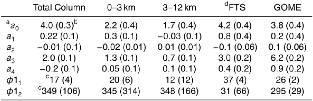
7, 14543–14568, 2007 Long-term tropospheric formaldehyde concentrations N. B. Jones et al. Title Page Abstract Introduction Conclusions References Tables Figures ◭ ◮ ◭ ◮ Back Close Full Screen / EscPrinter-friendly Version Interactive Discussion Table 3. The coefficients from Eq. (1), for the HCHO total column, partial columns 0–3 km and
3–12 km for the gb-FTS data while the right two columns contain the smoothed gb-FTS total column using the GOME averaging kernel and the GOME total column results respectively.
Total Column 0–3 km 3–12 km dFTS GOME
a a0 4.0 (0.3)b 2.2 (0.4) 1.7 (0.4) 4.2 (0.4) 3.8 (0.4) a1 0.22 (0.1) 0.3 (0.1) −0.03 (0.1) 0.8 (0.4) 0.2 (0.4) a2 −0.01 (0.1) −0.02 (0.01) 0.01 (0.01) −0.1 (0.06) 0.1 (0.06) a3 2.0 (0.1) 1.3 (0.1) 0.7 (0.1) 3.0 (0.2) 6.2 (0.2) a4 −0.2 (0.1) 0.05 (0.1) 0.1 (0.1) 0.4 (0.2) 0.9 (0.2) φ11 c17 (4) 20 (6) 12 (12) 37 (4) 26 (2) φ12 c349 (106) 345 (314) 348 (166) 31 (66) 295 (29) Notes: a
For all coefficients a0through a4the units are × 10 15
molecules cm−2. b
The numbers in brackets are the standard deviation.
c
For coefficients φ1and φ2the values are day of year. d
Smoothed gb-FTS total columns.
ACPD
7, 14543–14568, 2007 Long-term tropospheric formaldehyde concentrations N. B. Jones et al. Title Page Abstract Introduction Conclusions References Tables Figures ◭ ◮ ◭ ◮ Back Close Full Screen / EscPrinter-friendly Version Interactive Discussion Fig. 1. (a) The a priori HCHO mixing ratio profile used in all analysis, as well as the computation
of the averaging kernel function in Fig. 1b. This profile is based on measured aircraft profile measurements (NASA/PEM-Tropics B, (Singh et al., 2001). (b) Averaging kernels for the total column (0–100 km), 0–3 and 3–12 km partial columns for a solar zenith angle of 73.4◦. Also
shown (black dotted line) is the contribution of the a priori profile to the final retrieved solution.
ACPD
7, 14543–14568, 2007 Long-term tropospheric formaldehyde concentrations N. B. Jones et al. Title Page Abstract Introduction Conclusions References Tables Figures ◭ ◮ ◭ ◮ Back Close Full Screen / EscPrinter-friendly Version Interactive Discussion Fig. 2. The monthly mean HCHO total column amount for the years 1992 to 2005 (black
symbols). The error bars assume a total error of 16% per spectrum (Table 2) that is divided by the square root of the number of measurements per month. The blue line is a seasonal mean least squares fit to the data using Eq. (1).
ACPD
7, 14543–14568, 2007 Long-term tropospheric formaldehyde concentrations N. B. Jones et al. Title Page Abstract Introduction Conclusions References Tables Figures ◭ ◮ ◭ ◮ Back Close Full Screen / EscPrinter-friendly Version Interactive Discussion Fig. 3. The monthy mean HCHO partial columns and seasonal trend line for the 0–3 km (red
symbols and red line respectively) and 3–12 km (black symbols and black line respectively) layers. The error bars are based on the results from the full error analysis data in Table 2, while the seasonal trend lines are computed from the coefficients in Table 3.
ACPD
7, 14543–14568, 2007 Long-term tropospheric formaldehyde concentrations N. B. Jones et al. Title Page Abstract Introduction Conclusions References Tables Figures ◭ ◮ ◭ ◮ Back Close Full Screen / EscPrinter-friendly Version Interactive Discussion Fig. 4. Averaging kernels for GOME (blue line summer, red line winter) based on HCHO model
profiles from GEOS-Chem, with the gb-FTS kernels (solid black line total column, dotted black line 0–3 km) from Fig. 1 for direct comparison. The light gray vertical line at weight=1.0 is the “perfect” averaging kernel for reference.
ACPD
7, 14543–14568, 2007 Long-term tropospheric formaldehyde concentrations N. B. Jones et al. Title Page Abstract Introduction Conclusions References Tables Figures ◭ ◮ ◭ ◮ Back Close Full Screen / EscPrinter-friendly Version Interactive Discussion Fig. 5. A comparison of total columns from GOME (blue diamonds) that have been regridded
onto the spatial grid of the gb-FTS. The gb-FTS data (red diamonds) have been smoothed with the GOME averaging kernel (either summer or winter kernels, Fig. 4). Also plotted are seasonal fits, using Eq. (1), to the GOME data (solid blue line), smoothed gb-FTS (solid red line), and the fit of the “pre-smoothed” gb-FTS total column from Fig. 2. The fitting statistics are reported in Table 3. The vertical error bars are mean GOME errors derived from the original smoothed GOME data.
ACPD
7, 14543–14568, 2007 Long-term tropospheric formaldehyde concentrations N. B. Jones et al. Title Page Abstract Introduction Conclusions References Tables Figures ◭ ◮ ◭ ◮ Back Close Full Screen / EscPrinter-friendly Version Interactive Discussion Fig. 6. A correlation plot of the gb-FTS versus GOME from the data of Fig. 5. The solid line
is a linear fit to the gb-FTS and GOME data for reference. The dashed lines are 1 sigma error limits based on the mean error from the gb-FTS and GOME error statistics. The data points marked with a green star were excluded from the correlation calculation as outliers.