HAL Id: hal-01186044
https://hal.archives-ouvertes.fr/hal-01186044
Submitted on 29 Apr 2016
HAL is a multi-disciplinary open access
archive for the deposit and dissemination of
sci-entific research documents, whether they are
pub-lished or not. The documents may come from
teaching and research institutions in France or
abroad, or from public or private research centers.
L’archive ouverte pluridisciplinaire HAL, est
destinée au dépôt et à la diffusion de documents
scientifiques de niveau recherche, publiés ou non,
émanant des établissements d’enseignement et de
recherche français ou étrangers, des laboratoires
publics ou privés.
Distributed under a Creative Commons Attribution| 4.0 International License
superconductivity in the diffusive limit: application to
strongly spin-polarized systems
Matthias Eschrig, Audrey Cottet, Wolfgang Belzig, J. Linder
To cite this version:
Matthias Eschrig, Audrey Cottet, Wolfgang Belzig, J. Linder. General boundary conditions for
qua-siclassical theory of superconductivity in the diffusive limit: application to strongly spin-polarized
systems. New Journal of Physics, Institute of Physics: Open Access Journals, 2015, 17, pp.083037.
�10.1088/1367-2630/17/8/083037�. �hal-01186044�
This content has been downloaded from IOPscience. Please scroll down to see the full text.
Download details:
IP Address: 134.157.80.136
This content was downloaded on 29/04/2016 at 08:51
Please note that terms and conditions apply.
General boundary conditions for quasiclassical theory of superconductivity in the diffusive
limit: application to strongly spin-polarized systems
View the table of contents for this issue, or go to the journal homepage for more 2015 New J. Phys. 17 083037
PAPER
General boundary conditions for quasiclassical theory of
superconductivity in the diffusive limit: application to strongly
spin-polarized systems
M Eschrig1,2, A Cottet3, W Belzig4and J Linder2
1 Department of Physics, Royal Holloway, University of London, Egham, Surrey TW20 0EX, UK 2 Department of Physics, Norwegian University of Science and Technology, N-7491 Trondheim, Norway
3 Laboratoire Pierre Aigrain, Ecole Normale Supérieure-PSL Research University, CNRS, Université Pierre et Marie Curie-Sorbonne
Universités, Université Paris Diderot-Sorbonne Paris Cité, 24 rue Lhomond, F-75231 Paris Cedex 05, France
4 Department of Physics, University of Konstanz, D-78457 Konstanz, Germany
E-mail:matthias.eschrig@rhul.ac.uk
Keywords: superconducting spintronics, triplet supercurrents, boundary conditions
Abstract
Boundary conditions in quasiclassical theory of superconductivity are of crucial importance for
describing proximity effects in heterostructures between different materials. Although they have been
derived for the ballistic case in full generality, corresponding boundary conditions for the diffusive
limit, described by Usadel theory, have been lacking for interfaces involving strongly spin-polarized
materials, e.g. half-metallic ferromagnets. Given the current intense research in the emerging
field of
superconducting spintronics, the formulation of appropriate boundary conditions for the Usadel
theory of diffusive superconductors in contact with strongly spin-polarized ferromagnets for arbitrary
transmission probability and arbitrary spin-dependent interface scattering phases has been a burning
open question. Here we close this gap and derive the full boundary conditions for quasiclassical Green
functions in the diffusive limit, valid for any value of spin polarization, transmission probability, and
spin-mixing angles (spin-dependent scattering phase shifts). Our formulation allows also for complex
spin textures across the interface and for channel off-diagonal scattering (a necessary ingredient when
the numbers of channels on the two sides of the interface differ). As an example we derive expressions
for the proximity effect in diffusive systems involving half-metallic ferromagnets. In a
super-conductor/half-metal/superconductor Josephson junction we
find
ϕ
0-junction behavior under
certain interface conditions.
1. Introduction
Hybrid structures containing superconducting (S) and ferromagnetic (F) materials became a focus of
nanoelectronic research because of their relevance for spintronics applications as well as their potential impact on fundamental research [1–3]. Examples of successful developments include the discoveries of theπ-junction [4,5] in S/F/S Josephson devices [6,7], of odd-frequency superconductivity [8] in S/F heterostructures [9,10], and of the indirect Josephson effect in S/half-metal/S junctions [11,12]. Other recent topics of interest include the study of Majorana fermions at interfaces between superconductors and topological insulators [13] and at edges in superfluid3He[14,15], and the appearance of pure spin supercurrents in topological superconductors [16], and in S/FI-F-FI devices as a result of geometric phases [17].
The central subject in many of these studies is to understand how in the case of a superconductor coupled to a ferromagnetic material superconducting correlations penetrate into the ferromagnet, and how magnetic correlations penetrate into the superconductor [18–23]. A powerful method to treat such problems is the quasiclassical theory of superconductivity developed by Larkin and Ovchinnikov and by Eilenberger [24,25]. Within this theory [26–30] the quasiparticle motion is treated on a classical level, whereas the particle–hole and
OPEN ACCESS RECEIVED
22 April 2015
REVISED
22 June 2015
ACCEPTED FOR PUBLICATION
23 June 2015
PUBLISHED
18 August 2015
Content from this work may be used under the terms of theCreative Commons Attribution 3.0 licence.
Any further distribution of this work must maintain attribution to the author(s) and the title of the work, journal citation and DOI.
the spin degrees of freedom are treated quantum mechanically. The transport equation, which is afirst-order matrix differential equation for the quasiclassical propagator, must be supplemented by physical boundary conditions in order to obtain a unique solution.
Whereas for the full microscopic Green functions, i.e. the Gor’kov Green functions [31], such boundary conditions can be readily formulated (e.g. in terms of interface scattering matrices or in terms of transfer matrices), this is a considerably more difficult task for quasiclassical Green functions. In quasiclassical theory only the information about the envelope functions of Bloch waves is retained; information about the phases of the waves is missing. Such envelope amplitudes can show jumps at interfaces, and one complex task is to calculate these jumps without knowing the full microscopic Green functions near the interface.
Correspondingly, there is a long history of deriving boundary conditions for quasiclassical propagators, both for the Eilenberger equations, and their diffusive limit, the Usadel equations [32].
For ballistic transport, described by the Eilenberger equations, such boundary conditions werefirst formulated for spin-inactive interfaces in pioneering work by Shelankov and by Zaitsev [34,35], who showed the non-trivial fact that these jumps can be calculated using only the envelope functions. More general formulations were proposed subsequently [36–39], including a formulation in terms of interface scattering matrices by Millis, Rainer and Sauls [39]. All these formulations were implicit in terms of non-linear matrix equations, and problems arose in numerical implementations due to spurious (unphysical) additional solutions which must be eliminated. Progress was made with the help of Shelankov’s projector formalism [40], allowing for explicit formulations of boundary conditions in both equilibrium [41–43] and non-equilibrium [42] situations. Further generalizations included spin-active interfaces, formulated for equilibrium [44] and for non-equilibrium [45], and interfaces with diffusive scattering characteristics [46]. An alternative formulation in terms of quantum mechanical t-matrices [47] proved also fruitful [11,20,48–51]. The latest formulation, in terms of interface scattering matrices, is able to include non-equilibrium phenomena, interfaces and materials with weak or strong spin polarization, multi-band systems, as well as disordered systems [52].
For the diffusive limit a set of second-order matrix differential equations was derived by Usadel [32]. In contrast to the ballistic case, where boundary conditions have been formulated for a wide set of applications, boundary conditions for the diffusive limit have been formulated so far only in certain limiting cases. Thefirst formulation is by Kupriyanov and Lukichev, appropriate for the tunneling limit [53]. This was generalized to arbitrary transmission by Nazarov [54]. A major advance was done by Cottet et al in formulating boundary conditions for Usadel equations appropriate for spin-polarized interfaces [55]. These boundary conditions are valid in the limit of small transmission, spin polarization, and spin-dependent scattering phase shifts (this term is often used interchangeably with‘spin-mixing angles’ [56]). Subsequent formulations allowed for arbitrary spin polarization, although being restricted to small transmission and spin-dependent scattering [57–59]. In [59] the authors present‘heuristically’ deduced boundary conditions, which coincide with the ones used in [57,58].
Here we not only present the full derivation of the specific boundary conditions used in [57–59], but go further and give a full solution of the problem. With this, the long-standing problem of how to generalize Nazarov’s formula for arbitrary transmission probability [54] to the case of spin-polarized systems with arbitrary spin polarization and arbitrary spin dependent scattering phases is solved. Our boundary conditions are general enough to allow for non-equilibrium situations within Keldysh formalism, as well as for complex interface spin textures. We reproduce as limiting cases all previously known formulations.
2. Transport equations
The central quantity in quasiclassical theory of superconductivity [24,25] is the quasiclassical Green function (‘propagator’) gˇ ( , , , )pF R E t . It describes quasiparticles with energy E (measured from the Fermi level) and momentum pFmoving along classical trajectories with direction given by the Fermi velocity v pF( F)in external potentials and self-consistentfields that are modulated by the slow spatial (R) and time (t) coordinates [26–28]. The quasiclassical Green function is a functional of self-energiesΣˇ ( , , , )pF R E t , which in general include molecularfields, the superconducting order parameterΔ(pF,R, )t , impurity scattering, and the external potentials. The quantum mechanical degrees of freedom of the quasiparticles show up in the matrix structure of the quasiclassical propagator and the self-energies. It is convenient to formulate the theory using 2 × 2 matrices in Keldysh space [60] (denoted by a‘check’ accent), the elements of which in turn are 2 × 2 Nambu–Gor’kov matrices [31,61] in particle–hole (denoted by a ‘hat’ accent) space. The structure of the propagators and
g g g g a ˇ ˆ ˆ 0 ˆ , ˇ ˆ ˆ 0 ˆ , (1 ) R K A R K A kel kel ⎛ ⎝ ⎜⎜ ⎞⎠⎟⎟ Σ ⎛⎝⎜⎜Σ Σ ⎞⎠⎟⎟ Σ = =
where the superscripts R, A and K refer to retarded, advanced and Keldysh components, respectively, and with the particle–hole space structure5
g g f f g g g f f g b ˆ ˜ ˜ , ˆ ˜ ˜ (1 ) R A R A R A R A R A K K K K K , , , , , ph ph ⎛ ⎝ ⎜ ⎜ ⎞ ⎠ ⎟ ⎟ ⎛ ⎝ ⎜ ⎜ ⎞ ⎠ ⎟ ⎟ = = − −
for Green functions, and
c ˆ ˜ ˜ , ˆ ˜ ˜ (1 ) R A R A R A R A R A K K K K K , , , , , ph ph ⎛ ⎝ ⎜ ⎞ ⎠ ⎟ ⎛ ⎝ ⎜ ⎞ ⎠ ⎟ Σ Σ Δ Δ Σ Σ Σ Δ Δ Σ = = − −
for self-energies. For spin-degenerate trajectories (i.e. in systems with weak or no spin-polarization) the elements of the 2 × 2 Nambu-Gor’kov matrices are 2 × 2 matrices in spin space, e.g. gR g
ab R
= with
a b, ∈ ↑ ↓{ , }, and similarly for others. In strongly spin-polarized ferromagnets the elements of the 2 × 2 Nambu-Gor’kov matrices are spin-scalar (due to very fast spin-dephasing in a strong exchange field), and the system must be described within the preferred quantization direction given by the internal exchangefield. The terms‘weak’ and ‘strong’ refer to the spin-splitting of the energy bands being comparable to the superconducting gap or to the band width, respectively. In writing equations (1a)–(1c) we used general symmetries, which are accounted for by the‘tilde’ operation,
(
)
(
)
X˜ pF,R, ,E t = X −pF,R,−E t, * . (2)
Retarded (advanced) functions can be analytically continued into the upper (lower) complex energy half plane, in which case the relation is modified to X˜( , , , )pF R E t = X(−pF,R,−E*, )*t with complex E.
The quasiclassical Green functions satisfy the Eilenberger–Larkin–Ovchinnikov transport equation and normalization condition
Eˇ3 ˇ , ˇg i vF · gˇ 0ˇ, gˇ gˇ 21ˇ. (3)
⎡⎣ τ −Σ ⎤⎦ + = ◦ = −π
◦
The non-commutative product ◦ combines matrix multiplication with a convolution over the internal energy-time variables in Wigner coordinate representation,
(
Aˇ◦B E tˇ ( , ))
≡e2i(
∂ ∂ −∂ ∂AE tB tA EB)
A E t B E tˇ ( , ) ˇ ( , ), (4) and ˇτ3 = τˆ 1ˇ3 , whereτˆ3is a Pauli matrix in particle–hole space. Here and below, A B[ , ]◦ ≡A◦B−B◦A.The operation acts on the variable R.
The functional dependence of the quasiclassical propagator on the energies is given in the form of self-consistency conditions. For instance, for a weak-coupling, s-wave order parameter, the condition reads
(
)
t V E N f E t R p p R ˆ ( , ) d 4 i ( ) ˆ , , , , (5) s E E F F s K F p c c F∫
〈
〉
Δ π = −where Vsis the s-wave part of the singlet pairing interaction, NFis the density of states per spin at the Fermi level,
fˆsKis spin-singlet part of the the Keldysh component fˆK, and〈〉pFdenotes averaging over the Fermi surface. The
cut-off energy Ecis to be eliminated in favor of the superconducting transition temperature in the usual manner. When the quasiclassical Green function has been determined, physical quantities of interest can be
calculated. For example, the current density at position R and time t reads (with e<0the electron charge)
(
)
t e E N g E t j R( , ) d p v p p R 8 i Tr F( F) F( F) ˆ ˆ , , , . (6) K F p 3 F∫
〈
〉
π τ = −∞ ∞The symbol Tr denotes a trace over the 2 × 2 particle–hole space as well as over 2 × 2 spin space in the case of spin-degenerate trajectories.
In the dirty (diffusive) limit, strong scattering by non-magnetic impurities effectively averages the quasiclassical propagator over momentum directions. The Green function may then be expanded in the small parameter k TB cτ (τ is the momentum relaxation time) following the standard procedure [32,33]
5For the de
finitions of all Green functions in this paper we use a basis of fermion field operators in Nambu ⊗ spin-space as
t t t t t
r r r r r
( , ) [ ( , ), ( , ), ( , ) ,† ( , ) ]†T
(
)
(
)
gˇ pF,R, ,E t ≈Gˇ ( , , )R E t +gˇ(1) pF,R, ,E t (7) where the magnitude of gˇ(1)is small compared to that ofGˇ. The impurity self-energy is related to an (in general
anisotropic) lifetime functionτ(p′F,pF)[33]. Substitutings (7) into equation (3), multiplying with
N pF( ′F)v (F j, p′F) (τ p′F,pF), averaging over momentum directions, considering thatΣ τˇ′ is small, whereΣ′ˇ is the self-energy reduced by the contribution due to non-magnetic impurity scattering, and using
Gˇ ◦Gˇ = −π21ˇand Gˇ◦gˇ(1)+ gˇ(1)◦Gˇ = 0ˇ, one obtains (we suppress here the argumentsR, , )E t
N (p )v (p ) ˇ (g p ) N D G G i ˇ ˇ , (8) F F F j F F F k jk k p , (1) F
∑
π = ◦where NF = 〈N pF( F)〉pFis the local density of states per spin at the Fermi level,k = ∂ ∂Rk, the
summation is over k∈{ , , }x y z, and
( ) ( ) (
)
D N N p p p p p N p 1 v , v ( ) ( ) (9) jk F F F F j F F F F k F F F p p 2 , , F F τ = ′ ′ ′ ′is the diffusion constant tensor. For isotropic systems, Djk = Dδjk. The Usadel Green functionGˇobeys the
following transport equation and normalization condition, [32]
(
)
Eˇ ˇ , ˇG D Gˇ Gˇ 0ˇ, Gˇ Gˇ 1ˇ, (10) jk jk j k 3 0 2 ⎡⎣ τ Σ ⎤⎦∑
π π − + ◦ = ◦ = − ◦ whereΣˇ0 = 〈NF(pF) ˇ (Σ pF) pF NF′ 〉 . The Usadel propagatorGˇis a functional of ˇ
0
Σ .
The structures ofGˇand ˇΣ0are the same as in equations (1a)–(1c) (withGˇreplacinggˇand ˇΣ0replacing ˇΣ0).
Equation (2) is replaced by
X˜( , , )R E t = X( ,R −E t, )*. (11) The current density for diffusive systems is obtained from equations (8) and (6), and is given by
j( , )R t e dE N D G R E t G R E t 8 Tr ˆ ˇ ( , , ) ˇ ( , , ) . (12) i k F ik k K 2 3⎡⎣ ⎤⎦
∫
∑
π τ = − ◦ −∞ ∞A vector potentialA R( , ) enters in a gauge invariant manner by replacing the spatial derivative operators in allt
expressions by (see e.g. [33,62])
Xˆ ˆ Xˆ Xˆ i eˆ A X, ˆ . (13)
i i i ⎡⎣⎢ 3 i ⎤⎦⎥
→ ∂ ◦ ≡ − τ
◦
Finally, the case of a strongly spin-polarized itinerant ferromagnet with superconducting correlations (e.g. due to the proximity effect when in contact with a superconductor) can be treated by quasiclassical theory as well [11,20,50]. In this case, when the spin-splitting of the energy bands is comparable to the band width of the two spin bands, there exist two well-separated fully spin-polarized Fermi surfaces in the system, and the length scale associated with ∣pF↑−pF↓∣is much shorter than the coherence length scale in the ferromagnet. Equal-spin correlations stay still coherent over long distance in such a system;↑↓and↓↑correlations are, however, incoherent and thus negligible within quasiclassical approximation. Fermi velocity, density of states, diffusion constant tensor, and coherence length all become dependent. The quasiclassical propagator is then spin-scalar for each trajectory, with either all elements↑↑or all elements↓↓depending on the spin Fermi surface the trajectory corresponds to. Eilenberger equation and Usadel equation have the same form as before for each separate spin band. The spin-resolved current densities are given in the ballistic case by
e E N g j d v 8 i Tr F F ˆ ˆ , (14) K p 3 F
∫
π τ = ↑ −∞ ∞ ↑ ↑ ↑↑ ↑and in the diffusive case by
j e dE N D G G 8 Tr ˆ ˇ ˇ , (15) k k F kj j K 2 3⎡⎣ ⎤⎦
∫
∑
π τ = − ◦ ↑ −∞ ∞ ↑ ↑ ↑↑ ↑↑and analogously for spin down.
For heterostructures, the above equations must be supplemented with boundary conditions at the interfaces. A practical formulation of boundary conditions for diffusive systems valid for arbitrary transmission and spin polarization is the goal of this paper.
3. Boundary conditions
3.1. Interface scattering matrix
We formulate boundary conditions at an interface in terms of the normal-state interface scattering matrix Sˆ [63–65], connecting incoming with outgoing Bloch waves on either side of the interface with each other. We use the notation S S S S S ˆ ˆ ˆ ˆ ˆ , (16) 11 12 21 22 ⎛ ⎝ ⎜⎜ ⎞⎠⎟⎟ = − ⤧
where 1 and 2 refer to the two sides of the interface, and the subscript label⤧indicates that the 2 × 2 matrix structure refers to reflection and transmission amplitudes at an interface. The components Sˆijare matrices in
particle–hole space as well as in scattering channel space (i.e. scattering channels for ballistic transport would be parameterized by the Fermi momenta of incoming and outgoing Bloch waves). Each element in 2 × 2 particle– hole space is in turn a matrix in combined spin and channel space, i.e. the number of incoming directions (assumed to be equal to the number of outgoing directions due to particle conservation) gives the dimension in channel space. The dimension in spin space is for spin-degenerate channels 2 and for spin-scalar channels 1.
If time-reversal symmetry is preserved, Kramers degeneracy requires that each element of the scattering matrix has a 2 × 2 spin (or more general: pseudo-spin) structure (as it connects doubly degenerate scattering channels on either side of the interface). For spin-polarized interfaces (e.g. ferromagnetic or with Rashba spin– orbit coupling) the scattering matrix is not spin-degenerate. However if the splitting of the spin-degeneracy is on the energy scale of the superconducting gap, it can be neglected within the precision of quasiclassical theory of superconductivity. On the other hand, if the lifting of the spin-degeneracy of energy bands is comparable to the Fermi energy, the degeneracy of the scattering channels must be lifted as well in order to achieve consistency within quasiclassical theory. For definiteness, we denote the dependence on the scattering channels by indices
n n, ′:
Sˆ , (17)
nn
⎡⎣ ⎤⎦αβ
′
even for the ballistic case for which S[ˆ ]αβnn′ ≡ Sˆαβ(pF n, ,kF n, ′).
As shown in appendicesAandB, the scattering matrix for an interface can be written in polar decomposition in full generality as CC C C C C Sˆ 1 1 0 0 ˘ (18) † † † ⎛ ⎝ ⎜ ⎜ ⎞ ⎠ ⎟ ⎟ ⎛ ⎝ ⎜ ⎜ ⎞ ⎠ ⎟ ⎟ = − − − ⤧ ⤧
with unitary matricesand˘, and a transmission matrix C. All are matrices in particle–hole space, scattering channel space, and possibly (pseudo-)spin space. The above decomposition divides the scattering matrix into a Hermitian part and a unitary part. From this decomposition, we can define the auxiliary scattering matrix
Sˆ 0 0 ˘ , (19) 0 ⎛ ⎝ ⎜ ⎞ ⎠ ⎟ = ⤧
which retains all the phase information during reflection on both sides of the interface, and has zero transmission components. The decomposition is uniquely defined when there are no zero-reflection singular values (we will assume here that a small non-zero reflection always takes place for each transmission channel; perfectly transmitting channels can always be treated separately as the corresponding boundary conditions are trivial). For the matrix C we introduce the parameterization
(
)
C = 1+tt†−12 ,t (20)
(see appendixC) which is uniquely defined when all singular values of t are in the interval [0, 1](which is required in order to ensure non-negative reflection singular values). We define for notational simplification ‘hopping amplitude’ matrices
t˘ , t , (21)
12 21 †
πτ = πτ =
as well as unitary matrices
In terms of those, obviously the relation
S ( )S (23)
¯ ¯ † ¯
ταα = α ταα α
holds, where ( , ¯)α α ∈{(1, 2), (2, 1)}, and the labels 1 and 2 refer to the respective sides of the interface. Here, and below, the Hermitian conjugate operation involves a transposition in channel indices. The particle–hole structures of the surface scattering matrix and the hopping amplitude are given by,
( )
( )
S S S ˆ 0 0 ˜ , ˆ 0 0 ˜ , (24) † ph ¯ ¯ ¯ † ph ⎛ ⎝ ⎜ ⎜ ⎞ ⎠ ⎟ ⎟ ⎛ ⎝ ⎜ ⎜ ⎞ ⎠ ⎟ ⎟ τ τ τ = = α α α αα αα αα with S˜ S , ˜ , (25) nn nn¯ ¯ ¯ nn ¯ nn¯ ¯ ⎡⎣ ⎤⎦α = ⎡⎣ ⎤⎦α ⎡⎣ ⎤⎦ταα = ⎡⎣ ⎤⎦ταα ′ ′ ∗ ′ ′ ∗wheren¯andn¯′denote mutually conjugated channels, e.g. defined by pF n, ¯′≡ −kF n, ′and kF n, ¯≡ −pF n, . Finally,
the Keldysh structure of these quantities is
( )
S S S S S ˇ ˆ 0 0 ˆ ˆ 0 0 ˆ , (26) R A † kel kel ⎛ ⎝ ⎜ ⎜ ⎜ ⎞ ⎠ ⎟ ⎟ ⎟ ⎛ ⎝ ⎜⎜ ⎞ ⎠ ⎟⎟ = ≡ α α α α α( )
ˇ ˆ 0 0 ˆ ˆ 0 0 ˆ (27) R A ¯ ¯ ¯ † kel ¯ ¯ kel ⎛ ⎝ ⎜ ⎜ ⎞ ⎠ ⎟ ⎟ ⎛ ⎝ ⎜ ⎞ ⎠ ⎟ τ τ τ τ τ = ≡ αα αα αα αα αα(the additional Hermitian conjugate in these equations is due to the fact that advanced Green functions have the roles of‘incoming’ and ‘outgoing’ momentum directions interchanged compared to retarded Green functions; this is similar to the additional Hermitian conjugate appearing for hole components in particle–hole space). Thus, the Keldysh matrix structure for Sˇαandτˇαα¯is trivial (proportional to the unit matrix). The full
normal-state scattering matrix is diagonal in particle–hole and in Keldysh space, with reflection components
(
) (
)
S Sˇ 1 2ˇ ˇ 1 ˇ ˇ ˇ , (28) ¯ †¯ 1 2 ¯ †¯ π τ τ π τ τ = + − αα αα αα αα αα α −and with transmission components
(
)
Sˇ ¯ 1 2ˇ ¯ˇ†¯ 2 ˇ . (29) 1 ¯ π τ τ πτ = + αα αα αα αα −Note thatτˇαα¯connects incoming with outgoing Bloch waves per definition (as the scattering matrix does).
We will formulate the theory such that all equations are valid on either side of the interface. This allows us to drop the indices , ¯α αfor simplicity of notation by randomly choosing one side of the interface, and denoting quantities on the other side of the interface by underline. In particular, we will use
Sˇ≡Sˇ ,α Sˇ≡Sˇ ,α¯ τˇαα¯≡τˇ, τˇαα¯ ≡ τˇ
gˇα≡gˇ , gˇα¯≡ gˇ , Gˇα≡Gˇ , Gˇα¯≡ Gˇ , (30)
and so forth (seefigure1(a)). Also, from equation (23) we haveτˇ = S Sˇ ˇ ˇτ† .
3.2. General boundary conditions for diffusive systems
One main problem with boundary conditions for quasiclassical propagators is illustrated infigures1(b) and (c). In previous treatments [39,54,55] the starting point was a transfer matrix description, seefigure1(b), which required the elimination of so-called‘drone amplitudes’, which are propagators that mix incoming with outgoing directions. Here, we will employ a scattering matrix description, seefigure1(c), which, on the other hand, requires a similar elimination of Drone amplitudes, this time being propagators mixing the two sides of the interface. However, for an impenetrable interface this latter problem does not arise, a fact we will exploit.
The strategy to derive the needed boundary conditions is to apply a three-step procedure. In thefirst step, the problem of an impenetrable interface with the auxiliary scattering matrix defined in equation (19) is solved on each side of the interface [11]. For this step, the ballistic solutions for the envelope functions for the Gor’kov
propagators close to the interfaces should be expressed by the solutionsGˇof the Usadel equation. In a second step, these ballistic solutions (auxiliary propagators) are used in order tofind the full ballistic solutions for finite transmission by utilizing a t-matrix technique [11,20,48,50]. In the third andfinal step the matrix current will be derived from the ballistic solutions, which then enters the boundary conditions for the Usadel equations. We
will present explicit solutions for all three steps, such that the procedure describes effectively boundary conditions for the solutions of Usadel equations on either side of the interface.
We use for the auxiliary propagators the notation gˇ0o, gˇ0i,gˇo
0 and gˇ
i
0, where the upper index denotes the
direction of the Fermi velocity. Incoming momenta (index i) are those with a Fermi velocity pointing towards the interface, and outgoing momenta (index o) are those with a Fermi velocity pointing away from the interface. 3.2.1. Solution for impenetrable interface
We solvefirst for the auxiliary ballistic propagators fulfilling the impenetrable boundary conditions
gˇ0o S g Sˇ ˇ ˇ ,0i † gˇo S gˇ ˇ ˇ ,i S (31)
0 0
†
= =
implying matrix multiplication in the combined (Keldysh) × (particle–hole) × (combined scattering-channel and spin) space. For diffusive banks, it is necessary to connect the ballistic propagators gˇ0i o, with the isotropic solutions of the Usadel equation,Gˇ. The ballistic propagators gˇ0i o, and gˇi o
0
,, which characterize electronic
correlations next to the scattering barrier, depend on the electronic momentum. However, in the diffusive case, impurity scattering leads to momentum isotropization away from the scattering barrier. This process occurs in isotropization zones with a thickness corresponding to a few times the inelastic mean-free path of the materials; seefigure1(a). This scale is itself much smaller than the scale on which the isotropic diffusive Green functions evolve in the bulk of the materials, in the framework of the Usadel equations. Indeed, the Usadel equations involve a superconducting coherence length, which is typically much larger than the elastic mean-free path. Therefore, in order to describe disordered hybrid structures with Usadel equations, suitable boundary conditions should be expressed in terms of the values of the isotropic Green functionsGˇandGˇright at the beginning of the isotropization zones. To obtain such boundary conditions from equation (31), it is necessary to express the propagators gˇ0i o, and gˇi o
0
, in terms ofGˇandGˇ. This can be done by studying the spatial dependence
of the Gor’kov Green functions (or full Green functions without the quasiclassical approximation) in the isotropization zones (see [54,55] for details). Using the fact that the dynamics of electrons is dominated by
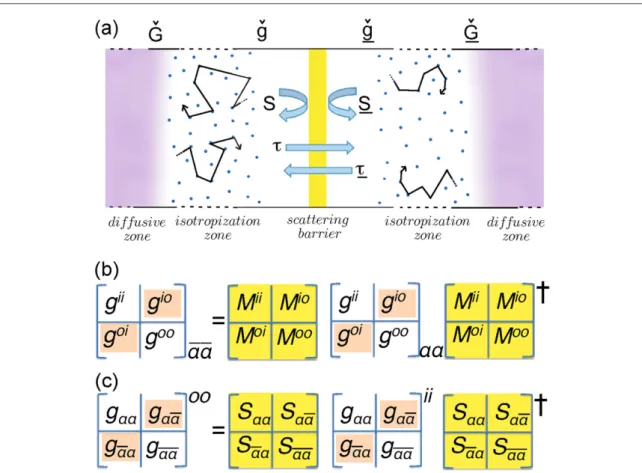
Figure 1. (a) Illustration of notation used in this paper. (b) and (c) Structure of boundary condition with transfer matricesMin (b), and with scattering matricesSin (c) (yellow).‘Drone’ amplitudes in the propagators (orange fields) connect in (b) incoming (i) and outgoing (o) momentum directions, and in (c) the two sides,α and α, of the interface. To obtain quasiclassical boundary conditions, Drone amplitudes in (b) and (c) must be eliminated. In this paper we use formulation (c). To connect to the notation in the main text,
gii ≡gi αα ,g g ii i ¯ ¯≡ αα ,g g oo≡ o αα , and g g oo o ¯ ¯≡ αα .
impurity scattering in these zones, one can express the Gor’kov Green functions in terms of gˇi o 0 ,, gˇi o 0 , ,GˇandGˇ. Then, an elimination of unphysical solutions imposes the conditions [54]
(
Gˇ−i 1ˇπ) (
◦ gˇ0i+i 1ˇπ)
= 0ˇ,(
gˇ0i−i 1ˇπ) (
◦ Gˇ +i 1ˇπ)
= 0ˇ (32 )a(
Gˇ +i 1ˇπ) (
◦ gˇ0o−i 1ˇπ)
= 0ˇ,(
gˇ0o+i 1ˇπ) (
◦ Gˇ −i 1ˇπ)
= 0ˇ (32 )band similarly forGˇand gˇi o
0
,. From this one obtains the identity1
{
gˇ , ˇi o G}
1ˇ2 0
, = −π2
◦ for the anticommutator
{…}. This allows to solve after some straightforward algebra for gˇ0i o,, using equation (31), and using the abbreviations
(
)
(
)
Gˇ 1 S GS G G SGS G 2 ˇ ˇ ˇ ˇ , ˇ 1 2 ˇ ˇ ˇ ˇ , (33) 2 † 2 † π π ′ = − ″ = −(both are matrices depending via Sˇ on the scattering channel index) leading to [55]
(
)
(
)
gˇ0i−i 1ˇπ = 1−Gˇ ◦Gˇ′−1◦ Gˇ −i 1ˇ ,π (34 )a
(
)
(
)
gˇ0o+i 1ˇπ = 1−Gˇ ◦Gˇ″ −1◦ Gˇ +i 1ˇπ (34 )b
(here and below the inverse is defined with respect to the ◦-product), which, using identities like
Gˇ Gˇ 1 { ˇ , ˇ}G G
2 2
′ ◦ ′ = − ′
π ◦ (with A B{ , }◦ ≡A◦B+B◦A), alternatively can be written also as
(
) (
)
gˇ0i+i 1ˇπ = Gˇ +i 1ˇπ ◦ 1−Gˇ′ ◦Gˇ −1, (34 )c
(
) (
)
gˇ0o−i 1ˇπ = Gˇ−i 1ˇπ ◦ 1−Gˇ″ ◦Gˇ −1. (34 )d
Similar equations hold forGˇand gˇi o
0
, in terms of the scattering matrix Sˇ. Introducing these solutions into
equations (32a) and (32b) shows readily that the latter are fulfilled. We note that the relation
gˇ0i o, ◦gˇ0i o, = −π21ˇfollows from Gˇ◦Gˇ = −π21ˇand SSˇ ˇ† = S Sˇ ˇ† = 1ˇ. It is also important to note that whereasGˇis proportional to the unit matrix in channel space due to their isotropic nature [55], Sˇ, and
consequentlyGˇ′, Gˇ″, and gˇ0i o,, are in general non-trivial matrices in channel space. Equations (34a) and (34b), or alternatively (34c) and (34d), together with equation (33) determine uniquely gˇ0i o, in terms of the diffusive Green functionGˇ. We can rewrite the difference gˇo gˇi
0 − 0in a more explicit manner, using the abbreviations
G G
ˇ ˇ ˇ
δ′ ≡ ◦ ′andδ″ ≡ˇ Gˇ″ ◦Gˇ, leading to
(
)
(
)
(
)
(
)
gˇ0o−gˇ0i = 1ˇ− ′δˇ −1◦⎡⎣ Gˇ −i 1ˇπ ◦ ″ − ′ ◦δˇ δˇ Gˇ−i 1ˇπ ⎦⎤◦ 1ˇ− ″δˇ −1. (35)
3.2.2. Solution forfinite transmission
The second step follows [11,20]. Once the auxiliary propagators are obtained, the full propagators can be obtained directly, without further solving the transport equation, in the following way. We solve t-matrix equations resulting from the transmission parameters ˇτ, for incoming and outgoing directions, which according to a procedure analogous to the one discussed in [47,48] take the form,
(
)
(
)
tˇi ˇ† gˇo ˇ 1ˇ gˇi tˇ ,i tˇo ˇ ˇgi ˇ 1ˇ gˇo ˇ .to (36) 0 0 0 † 0 τ τ τ τ = ◦ + ◦ = ◦ + ◦Using the symmetry equation (23), the t-matrices for incoming and outgoing directions can be related through
tˇo = S t Sˆ ˇ ˆ .i † (37)
Using the short notation
gˇ1o ˇ ˇgi ˇ , gˇi ˇ gˇo ˇ, (38) 0 † 1 † 0 τ τ τ τ ≡ ≡
we solve formally equations (36) fortˇi o,:
(
)
tˇi o, = 1−gˇ1i o, ◦gˇ0i o, −1◦gˇ .1i o, (39)
The full propagators, fulfilling the desired boundary conditions at the interface, can now be easily calculated. For incoming and outgoing directions they are obtained from [11,50]
(
)
(
)
gˇi gˇi gˇi i 1ˇ tˇi gˇi i 1ˇ , (40 )a
0 0 π 0 π
(
)
(
)
gˇo gˇo gˇo i 1ˇ tˇo gˇo i 1ˇ . (40 )b
0 0 π 0 π
= + − ◦ ◦ +
Noticing that
(
gˇ0i o, +i 1ˇπ) (
◦ gˇ0i o, −i 1ˇπ)
= 0ˇ, and(
gˇ0i o, −i 1ˇπ) (
◦ gˇ0i o, +i 1ˇπ)
= 0ˇ, as well as identities like gˇ0i o, ◦( ˇg0i o, + i 1ˇ)π = i 1ˇπ ◦( ˇg0i o, +i 1ˇ)π etc, it is obvious that the normalization gˇi o, ◦gˇi o, = −π21ˇ holds. Using the same identities, we obtain the alternative to equations (40a) and (40b) expressions(
)
(
)
gˇi gˇi gˇi i 1ˇ t gˇ , ˇi i gˇi t gˇ , ˇi i gˇi i 1ˇ , (40 )c 0 0 π ⎡⎣ 0⎤⎦ 0 ⎡⎣ 0⎤⎦ 0 π = + + ◦ = − ◦ − ◦ ◦(
)
(
)
gˇo gˇo gˇo i 1ˇ tˇ , ˇo go gˇo tˇ , ˇo go gˇo i 1ˇ . (40 )d 0 0 π ⎡⎣ 0⎤⎦ 0 ⎡⎣ 0⎤⎦ 0 π = + − ◦ = − ◦ + ◦ ◦Equations (40a) and (40b), or alternatively, (40c) and (40d), in conjunction with equations (38) and (39), solve the problem offinding the ballistic solutions for finite transmission. We are now ready for the last step, to relate these solutions to the matrix current which enters in the expression for boundary conditions forGˇandGˇ. 3.2.3. Matrix current and boundary conditions for diffusive propagators
We now turn to the third,final, step. As shown in [54,55], the boundary conditions for quasiclassical isotropic Green functions can be obtained from the conservation of the matrix currentin the isotropization zones surrounding the scattering barrier. This quantity contains physical information on theflows of charge, spin and electron–hole coherence in a structure. We refer the reader to [54,55] for the general definition ofin terms of the Gor’kov Green functions. Using this definition, one can verify thatis spatially conserved along the entire isotropization zones. Then, one can expressnext to the scattering barrier in terms of the propagatorsgˇi o, and
gˇi o, , and at the beginning of the isotropization zones in terms ofGˇandGˇ, seefigure1(a). The conservation of
the matrix current provides an equality between the two expressions. Sincegˇi o, can be expressed in terms of gˇi o
0 ,
and gˇi o
0 ,
, and these in terms of theGˇandGˇ, this gives the desired boundary conditions. Following [50], after some straightforward algebra we obtain
(
)
(
)
tˇ , ˇo g0o 1 gˇ1o gˇ0o 1 gˇ , ˇ1o g0o 1 gˇ0o gˇ1o 1. (41) ⎡⎣ ⎤⎦ = − ◦ ⎡⎣ ⎤⎦ − ◦ ◦ − ◦ −Using relations (31) and (37) above, wefind
(
)
(
)
gˇi Sˇ† gˇo gˇo i 1ˇ tˇo gˇo i 1ˇ Sˇ, (42) 0 0 0 ⎡ ⎣ π π ⎤⎦ = + + ◦ ◦ −which allows to derive the following relation
g Sg S t g ˇ ˇo ˇ ˇ ˇi † 2 i ˇ , ˇo o . (43) 0 ⎡⎣ ⎤⎦ ′ ≡ − = − π ◦
For calculating the charge current density in a given structure, it is sufficient to know ˇ′, because the matrices Sˇ andSˇ†drop out of the trace as they commute with theτˆ3matrix in particle–hole space.
Finally we relate the obtained propagatorsgˇi o, to the matrix current,
g g ˇ ˇo ˇi ˇ ˇ (44) ≡ − ≡ ′ + ″ with Sg S g ˇ ˇ ˇ ˇi † ˇ .i (45) ″ ≡ −
We remind the reader here that ˇhas a matrix structure in Keldysh space, in particle–hole space, and in combined scattering-channel and spin space. In terms ofˇthe boundary condition results then from equation (8) and from the matrix current conservation in the isotropization regions [54]
G zG ˇ i ˇ d d ˇ , (46) q n nn 1 2
∑
π σ π = − ◦ =where z is the coordinate along the interface normal (away from the interface), n is a scattering channel index ( channels, spin-degenerate channels count as one), e N D2
F
σ = refers to the conductivity per spin, is the surface area of the contact, andqis the quantum of conductance, =q e2 h. The number of scattering
channels is expressed in terms of the projection of the Fermi surfaces on the contact plane,AF z, , by
AF z, (2 )2
= π . For isotropic Fermi surfaces AF z, = πkF2. In general,
k 1 d (2 ) , (47) n 1 A 2 2 F z,
∫
∑
π … = … = ∣∣4. Special cases
4.1. Spin-scalar and channel-diagonal case
The transition to the diffusive Green functions is trivial for the case of Sˆ = 1ˆ, as then gˇi gˇo Gˇ
0 = 0 = . If we
start from equation (41) in conjunction with equation (38), we obtain in the case of a spin-scalar and channel-diagonal matrixτˆnnwith the notation Gˇ = −i ˇπG
(
{
}
)
z a G G G G G G 2 ˇ i 4 ˇ , ˇ 4 ˇ , ˇ 2 2 ˇ d d ˇ (48 ) n nn n n n q ⎡⎣ ⎤⎦ ∑
∑
π σ = + − = ◦ withσ =e N D2 F and(
)
b 4 1 . (48 ) n nn nn 2 2 2 2 2 π τ π τ = ∣ ∣ + ∣ ∣ This reproduces Nazarov’s boundary condition [50,54].4.2. Case for interface between superconductor and ferromagnetic insulator
For the case of zero transmission, ˇτ ≡0ˇ, we canfind a closed solution if we assume that we can find a spin-diagonal basis for all reflection channels. For a channel-spin-diagonal scattering matrix we write Sˇnn e ein i ˇ
n
2
= φ ϑκ
withκˇ = diag
{
m⃗ ⃗σ,m⃗ ⃗ , where mσ*}
⃗2 = 1(leading toκˇ2 = 1). In this case we have gˇi o, gˇi o0 ,
= . We use equation (35), which straightforwardly leads to
(
)
(
)
(
)
(
)
G G G G G G G G G G G 2 ˇ i 1ˇ i sin 2 ˇ ˇ ˇ ˇ sin 2 2 ˇ ˇ ˇ ˇ 1ˇ i sin ˇ , ˇ sin 2 ˇ ˇ ˇ , ˇ 1ˇ i sin 2 ˇ ˇ ˇ ˇ sin 2 2 ˇ ˇ ˇ ˇ 1ˇ (49) n nn n n n n n n n 2 1 2 2 1 ⎡ ⎣ ⎢ ⎢ ⎢ ⎤ ⎦ ⎥ ⎥ ⎥ ⎧ ⎨ ⎩ ⎡⎣ ⎤⎦ ⎡⎣ ⎤⎦ ⎫ ⎬ ⎭ ⎡ ⎣ ⎢ ⎢ ⎢ ⎤ ⎦ ⎥ ⎥ ⎥ ∑
∑
π ϑ κ κ ϑ κ κ ϑ κ ϑ κ κ ϑ κ κ ϑ κ κ = − − + − × − + × − − + − − −(where we recall that Gˇ2 = 1ˇ). Note thatφndrops out, and only the spin mixing angleϑnmatters. Equation (49)
generalizes the results of [55] to arbitrary spin-dependent reflection phases. Further below we will give a physical
interpretation of the leading order terms arising in an expansion for smallϑn.
4.3. Exact series expansions
We now provide explicit series expansions for all quantities which will be useful for deriving formulas for various limiting cases. We start with writing the scattering matrix as Sˇ = ei ˇKwith hermitian Kˇ due to unitarity of Sˇ, i.e. Kˇ = Kˇ†. Then we use an expansion formula for Lie brackets in order to obtain the series expansion
S GS G m K G ˇ ˇ ˇ e ˇ e ( i) ! ˇ , ˇ (50) K K m m m † i ˇ i ˇ 0 ⎡⎣ ⎤⎦
∑
= − = − = ∞with the definitions K G⎡⎣ˇ , ˇm ⎤⎦ = ⎡⎣Kˇ , ˇ ,⎡⎣Km 1− Gˇ⎤⎦⎤⎦and K G⎡⎣ˇ , ˇ0 ⎤⎦ = .WiththisweobtainfromGˇ
equation (33) G m K G G m K G ˇ 1 2 ( i) ! ˇ , ˇ , ˇ 1 2 i ! ˇ , ˇ , (51) m m m m m m 2 1 2 1 ⎡⎣ ⎤⎦ ⎡⎣ ⎤⎦
∑
∑
π π ′ = − ″ = = ∞ = ∞which are very useful if Kˇ has a small pre-factor. Note also the identity Gˇ ◦⎡⎣K Gˇ , ˇ⎤⎦◦Gˇ = π2⎡⎣K Gˇ , ˇ⎤⎦.
Furthermore, from equations (34c) and (34d) wefind
(
)
gˇi Gˇ Gˇ i 1ˇ ( ˇG Gˇ) (52 )a l l 0 1∑
π = + + ◦ ′ ◦ = ∞(
)
gˇo Gˇ Gˇ i 1ˇ ( ˇG Gˇ .) (52 )b l l 0 1∑
π = + − ◦ ″ ◦ = ∞From equation (41), and using equations (31), (37), we derive
(
)
(
)
tˇ , ˇo go gˇ gˇ gˇ , ˇg gˇ gˇ , (53 )a k n o o k o o o o n 0 , 0 1 0 1 0 0 1 ⎡⎣ ⎤⎦ =∑
◦ ◦⎡⎣ ⎤⎦ ◦ ◦ ◦ = ∞ ◦(
)
(
)
t gˇ , ˇi i gˇ gˇ gˇ , ˇg gˇ gˇ , (53 )b k n i i k i i i i n 0 , 0 1 0 1 0 0 1 ⎡ ⎣ ⎤⎦ =∑
◦ ◦⎡⎣ ⎤⎦ ◦ ◦ ◦ = ∞ ◦which is useful if the transmission amplitudes ˇτ entering into gˇ1i o, are small. Finally, we obtain from equations (43) and (45) t g m K g ˇ 2 i ˇ , ˇ , ˇ i ! ˇ , ˇ . (54) o o m m m i 0 1 ⎡⎣ ⎤⎦ ⎡⎣ ⎤⎦ ′ = − π ″ =
∑
◦ = ∞Here, gˇiis obtained from
(
)
gˇi i 1ˇ Gˇ i 1ˇ ( ˇG Gˇ) 1ˇ t gˇ , ˇ . (55) l l i i 0 0 ⎜ ⎟ ⎛ ⎝ ⎡⎣ ⎤⎦ ⎞ ⎠∑
π π + = + ◦ ′ ◦ ◦ + = ∞ ◦4.4. Boundary condition for spin-polarized surface to third order in spin-mixing angles
Wefirst treat the case whentˇi o, ≡0ˇ, for example the case where one side of the junction is a ferromagnetic insulator (FI). Then
(
)
m K G m K G G G ˇ i ! ˇ , ˇ i ! ˇ , ˇ i 1ˇ ( ˇ ˇ) . (56) m m m m l m m l 1 , 1 ⎡⎣ ⎤⎦ ⎡⎣⎢ ⎤⎦⎥ =∑
+∑
+ π ◦ ′ ◦ = ∞ = ∞To third order we have ˇ = ˇ(1)+ˇ(2)+ ˇ(3), and the derivation in appendixDleads to
K G KGK G a ˇ i ˇ , ˇ , ˇ i 2 ˇ ˇ ˇ , ˇ (57 ) (1) (2) ⎡⎣ ⎤⎦ ⎡⎣ ⎤⎦ π = = − ◦ K G K G K G G b ˇ i 24 ˇ , ˇ i 8 ˇ , ˇ ˇ , ˇ ˇ . (57 ) (3) 3 2 2 ⎡⎣ ⎤⎦ ⎡ ⎣ ⎡⎣ ⎤⎦ ⎤⎦ π = − − ◦ ◦
For the special case of channel diagonal Kˇnn = 2nκˇ
ϑ
withκˇ2 = 1ˇ, which follows also from directly expanding
equation (49), we reproduce the results from [55] (Gˇ = −i ˇπG),
(
)
G G G a 2 ˇ i i ˇ , ˇ , 2 ˇ i 4 ˇ ˇ ˇ , ˇ (58 ) n nn n n n nn n n (1) (2) 2 ⎡⎣ ⎤⎦ ⎡⎣ ⎤⎦ ∑
∑
∑
∑
π ϑ κ π ϑ κ κ = − = ◦ b G G G G 2 ˇ i i 16 1 3 ˇ , ˇ ˇ ˇ ˇ ˇ ˇ, ˇ . (58 ) n nn n n (3) 3 ⎜ ⎟ ⎛ ⎝ ⎡⎣ ⎤⎦ ⎡⎣ ⎤⎦ ⎞⎠ ∑
∑
π ϑ κ κ κ κ = − − ◦ ◦Note that thefirst order term∼[ ˇ, ˇ ]κ G accounts for the effective exchangefield induced inside the
superconductor by the spin-mixing, whereas the term∼[ ˇ ˇ ˇ, ˇ ]κ κG G produces a pair breaking effect similar to that of paramagnetic impurities [66]. This second term occurs only at second order inϑnbecause it requires multiple
scattering at the S/FI interface, which together with random scattering in the diffusive superconductor leads to a magnetic disorder effect.
4.5. Boundary condition for spin-polarized interface to second order in spin-mixing angles and transmission probability
We now allow forfinite transmission, and concentrate on the matrix current to second order in the quantities Kˇ,
Kˇ, and gˇ1i o,. We need to take care of the scattering phases during transmission events. For this, we define
S S S S ˇ ˇ ˇ ˇ ,0 ˇ ˇ ˇ ˇ .0 (59) 1 2 1 2 1 2 1 2 τ = τ τ = τ
We note that equation (23), orτˇ = S Sˇ ˇ ˇτ† , results into
ˇ0 ˇ .0† (60)
τ = τ
Thus, theτˇ0andτˇ0are the appropriate transmission amplitudes, with transmission spin-mixing phases
Gˇ1≡τ0Gˇτ0†. (61) We expand ˇτ up tofirst order in Kˇ andKˇ,
(
K K)
ˇ ˇ i
2 ˇ ˇ ˇ ˇ , (62)
0 0 0
τ = τ + τ +τ + …
and obtain ˇ = ˇ(1)+ˇ(2)from a systematic expansion to second order in Kˇ , Kˇ, and Gˇ1, as shown in
appendixE, leading to one of the main results of this paper:
G G K G a ˇ(1) 2 i ˇ , ˇ i ˇ , ˇ , (63 ) 1 ⎡⎣ ⎤⎦ ⎡⎣ ⎤⎦ = − π + ◦ G G G G KGK G G GK KG G G K G G b ˇ 2 i ˇ ˇ ˇ , ˇ i 2 ˇ ˇ ˇ , ˇ i ˇ ˇ ˇ ˇ ˇ ˇ ˇ ˇ ˇ , ˇ ˇ , ˇ . (63 ) (2) 1 1 1 1 0 0† ⎡⎣ ⎤⎦ ⎡⎣ ⎤⎦ ⎡ ⎣ ⎡⎣ ⎤⎦ ⎤⎦ π π τ τ = − ◦ ◦ − + ◦ + ◦ + ◦ ◦ ◦ ◦
These relations generalize the results of [55] for the case of arbitrary spin polarization, and are valid even when
Kˇ ,Kˇandτ have different spin quantization axes, i.e. cannot be diagonalized simultaneously.
Using the notation Gˇ = −i ˇπGand2 ˇπτ0 = Tˇ, we can rewrite the result in leading order in the
quantities Kˇ , Kˇ, and the transmission probability ( TT∼ˇ ˇ†) as
T G T K G a 2 ˇ i ˇ ˇ ˇ 2i ˇ , ˇ , (64 ) (1) † ⎡ ⎣⎢ ⎤⎦⎥ π = − ◦
and for the next-to-leading order
T T T T K K T T K K T T T K T b G G G G G G G G G G G G G 2 ˇ i 1 4 ˇ ˇ ˇ ˇ ˇ ˇ ˇ , ˇ ˇ ˇ ˇ , ˇ i 2 ˇ ˇ ˇ ˇ ˇ ˇ ˇ ˇ ˇ ˇ ˇ ˇ ˇ , ˇ ˇ , ˇ . (64 ) (2) † † † † † ⎡ ⎣⎢ ⎤⎦⎥ ⎡⎣ ⎤⎦ ⎡ ⎣⎢ ⎡⎣ ⎤⎦ ⎤⎦⎥ π = − ◦ ◦ + + ◦ + ◦ + ◦ ◦ ◦ ◦
These equations are still fully general with respect to the magnetic (spin) structure, and allow for channel off-diagonal scattering as well as different numbers of channels on the two sides of the interface. Note that Tˇ , Kˇ , and
Kˇare matrices in channel space, whereas Gˇ and Gˇ are proportional to the unit matrix in channel space. Whereas
Kˇ , andKˇare square matrices, Tˇ in general can be a rectangular matrix (when the number of channels on the
two sides of the interface differ).
4.6. Boundary conditions for channel-independent spin quantization direction
As an application, we assume next that each of the quantities Kˇ ,Kˇ, andτˇ0can be spin-diagonalized
simultaneously for all channels, with spin quantization directions m⃗′, m⃗′, and m⃗ for Kˇ ,Kˇ, orτˇ0, respectively.
We also use that Gˇ and Gˇ are proportional to the unit matrix in channel space, as they are isotropic [55], and we assume that the number of channels on both sides of the interface are equal. We define
m T a 1ˇ · ˇ ˇ , (65 ) nl nl nl 0, + 1, ⃗ σ⃗ = m K m K b 1ˇ 1 2 · ˇ ˇ , 1ˇ 1 2 · ˇ ˇ , (65 ) nn nn nn ll ll ll φ ′ + ϑ ′ ⃗′ σ⃗ = ′ φ ′ + ϑ′ ⃗′ σ⃗ = ′ m m m c ˇ ˆ 1ˇ, ˆ 0 0 * ph, ˇ · ˇ , ˇ · ˇ , ˇ · ˇ (65 ) ⎛ ⎝ ⎜ ⎞ ⎠ ⎟ σ σ σ σ σ κ σ κ σ κ σ ⃗ = ⃗ ⃗ = ⃗ ⃗ ≡ ⃗ ⃗ ′ ≡ ⃗′ ⃗ ′ ≡ ⃗′ ⃗
with m⃗2 = (m⃗′)2 = (m⃗′)2 = 1, i.e. ˇκ2 = ( ˇ )κ′2 = ( ˇ )κ′2 = 1ˇ, and introduce the transmission
probabilitynland the spin polarization asnl
(
1ˇ mˇ)
Tˇ Tˇ . (66)nl nl nl nl
†
⎡⎣ ⎤⎦
+ ⃗ ⃗σ =
We write for0,nland1,nl, allowing for some spin-scalar phasesψnl,
2 1 1 e , 2 1 1 e . (67) nl nl nl nl nl nl 0, 2 2 2i 1,2 2 2i nl nl ⎡ ⎣ ⎤⎦ ⎡⎣ ⎤⎦ = + − ψ = − − ψ
We will average over all spin-scalar phasesψnlof the transmission amplitudes as there are usually many scattering channels in an area comparable with the superconducting coherence length squared. Thisfilters out all the terms in equations (64a) and (64b) where these scalar scattering phases cancel.
For a magnetic system, in linear order innlandϑnn′we obtain
(
)
(
)
I G G G 2 ˇ i 1ˇ ˇ ˇ 1ˇ ˇ , ˇ i ˇ , ˇ , (68) q n nn q nl nl nl nl nl q n nn (1) (1) 0, 1, 0,* 1,* ⎡ ⎣ ⎤⎦ ⎡⎣ ⎤⎦ ∑
∑
∑
π κ κ ϑ κ ≡ = + + − ′ where =q e2 his the conductance quantum. After multiplying out we obtain the set of boundary
conditions
{
}
I G G G G a 2 (1) ⎡ 0ˇ MR ˇ , ˇ 1ˇ ˇ ˇ i ˇ , ˇ (69 ) ⎣ κ κ κ κ ⎤⎦ = + + − ϕ ′ ◦ with(
1 1)
(69 )b q nl nl nl 0 2 = ∑
+ −(
1 1)
(69 )c q nl nl nl 1 2 = ∑
− − d , 2 (69 ) q nl nl nl q n nn MR = ∑
ϕ = ∑
ϑFor κ = κ′and the assumption of a channel-diagonal scattering matrix (n = l) this also provides the derivation of the boundary conditions used for [57]. We now proceed to the second-order terms:
{
}
(
)
(
)
(
)
{
}
{
}
I I a G G M M M G M G G G G G G M G G G G G G M G G G G G G 2 2 ˇ ˇ ˇ , ˇ i ˇ ˇ ˇ , ˇ ˇ ˇ ˇ ˇ ˇ ˇ ˇ ˇ ˇ , ˇ ˇ ˇ ˇ ˇ ˇ ˇ ˇ ˇ ˇ ˇ ˇ ˇ ˇ ˇ , ˇ ˇ ˇ ˇ , ˇ ˇ ˇ ˇ ˇ ˇ , ˇ ˇ , ˇ ˇ , ˇ (70 ) (2) 4 2 , 0 , 1 , MR , 0 0 0 , 1 1 1 , MR MR MR ⎡⎣ ⎤⎦ ⎡⎣ ⎤⎦ ⎡⎣ ⎤⎦ ⎡⎣ ⎤⎦ ⎡⎣ ⎤⎦ κ κ κ κ κ κ κ κ κ κ κ κ κ κ κ κ κ κ κ κ = − + ′ ′ + + + = ◦ ′ + ′ ◦ + ◦ ′ = ◦ ′ + ′ ◦ + ◦ ′ = ◦ ′ + ′ ◦ + ◦ ′ ϕ χ χ χ χ χ χ χ χ χ χ χ χ χ χ χ χ χ χ ◦ ◦where I4denotes a cumbersome expression in fourth order of the transmission amplitudes, which we do not write down here explicitly (see appendixF). We have used the abbreviations
(
)
b 1 4 q nl nn nl 1 1 nl (70 ) 0 2 χ= ∑
ϑ + −(
)
c 1 4 q nl nn nl 1 1 nl (70 ) 1 2 χ= ∑
ϑ − − d 1 4 , 1 2 (70 ) q nl nn nl nl q nn nn MR 2 2 χ = ∑
ϑ ϕ = ∑
ϑ ′ ′and0χ,1χ,MRχ are defined as0χ,1χ, andMRχ withϑnnreplaced byϑll. Note thatφnn′andφll′do not appear
in these expressions, in accordance with the intuitive notion that scalar scattering phases should drop out in the quasiclassical limit, which operates with envelope functions only.
The case for only channel-conserving scattering (channel-diagonal problem) follows by taking in equations (69b)–(69d) and (70b)–(70d) only the terms with n = l. All other formulas (69a), (70a) remain unchanged. This case is treated in [55] to linear order in , and our formulas reduce to these results for thenn
considered limit. Note that for this case all spin-scalar phases cancel automatically and no averaging procedure over these phases is necessary.
5. Application for diffusive superconductor/half metal heterostructure
The problem of a superconductor in proximity contact with a half-metallic ferromagnet has been studied within the frameworks of Eilenberger equations [11,12,20,50,52,67–69], Bogoliubov–de Gennes equations [70–73], recursive Green function methods [74], circuit theory [75], within a magnon-assisted tunneling model [76], and in the quantum limit [77]. Various experiments on superconductor/half-metal devices have been reported, both for layered systems involving high-temperature superconductors [78–81] and in diffusive structures involving conventional superconductors [82–88]. An important consequence of the new boundary conditions in equation (69a) is that half-metals can now be incorporated in the Usadel equation, which is appropriate to describe the second class of experiments mentioned above, whereas there previously existed no suitable boundary conditions to do so. Considerfirst a superconductor/half-metal bilayer with the interface located at x = 0 (seefigure2).
The superconductor is assumed to have a thickness well exceeding the superconducting coherence length. Our expansion parameters are the spin-dependent reflection phase shifts at the superconducting side of the interface,ϑll′, and the tunneling probabiliesnl. For calculating triplet components in the half-metal it is
sufficient to expand the solution for the Green function in the superconductor up to linear order, and the solution for the Green function in the half-metal up to quadratic order. The zeroth order term in the superconductor is pure spin-singlet, and thefirst-order term pure spin-triplet. Thus, up to and including the first order we can assume a bulk singlet order parameter, not affected by the interface scattering (corrections to the singlet order parameter arise only in second order inϑll′andnl). For future reference, we define the
quantities c≡cosh( )ν = −iE
Ω, s≡ sinh( )ν = i Δ Ω
∣ ∣
withν = atanh(∣ ∣Δ E),Ω = ∣Δ∣ −2 E2, and
denote the SC phase asθ. We find for the triplet componentFt 0in the superconductor
(
)
F x cs q m ( ) i e e · i (71) t0 q x y SC i σ σ σ = ⃗′ ⃗ ϕ θ − ∣ ∣with the normal-state conductivityσSC = 2e N D2 SC SCin the superconductor (NSCand DSCare the
normal-state density of normal-states per spin projection at the Fermi level and the diffusion constant, respectively), contact area
, and q = 2Ω DSC.
In the half-metal (width d), onlyspin‐↑particles have a non-zero density of states at the Fermi level. In the spirit of quasiclassical theory of superconductivity, a strong exchangefield is incorporated not in the transport equation, but directly in the band structure which is integrated out at the quasiclassical level [17,69], leaving only parameters such as the diffusion constant and normal state density of states at the Fermi level for each itinerant spin band. For transport in a half-metallic ferromagnet, this means one must just include one spin-band with diffusion constant DHMin the Usadel equation. Thus, only the elementsG↑↑andF↑↑exist in the
Green function Gˇ of the half-metal. As we expand in the tunneling probability, we can (for energies well exceeding the Thouless energy D HM d2of the half-metal) use the linearized Usadel equation,
DHM∂x2F↑↑+2iEF↑↑ = 0. (72)
Since there is only one anomalous Green function in the half-metal, we omit the spin indices for brevity of notation and define F≡ F↑↑. The general solution is F x( ) = Aeikx +Be−ikxwith A B, being complex
coefficients to be determined from the boundary conditions, and k = 2iE D HM. At the vacuum edge of the
half-metal x( = d), we have∂xF = 0. At the interface between the superconductor and half-metal, the
boundary conditions for F from the half-metallic side is obtained from equations (69a)–(70d) with = .nl 1 Note that for = , we havenl 1 0χ = 1χ = MRχ ≡χas well as0 = 1 = MR. Wefind that in
order to obtain a non-vanishing proximity effect, it is necessary that the magnetization direction associated with transmission across the barrier ( ˇκ) and spin-dependent phase-shifts picked up on the superconducting side of the interface ( ˇ )κ′ are different. We set ˇκ = σˇzsince the barrier magnetization determining the transmission
properties is expected to be dominated by the half-metal magnetization which points in the z-direction. The boundary condition for F at x = 0 reads:
(
)
F cs m m q 2i e i , 2 (73) x x y HM i 0 SC σ σ ∂ = ϑ θ ′ − ′ ϑ = χ+ ϕwith the normal-state conductivityσHM = e N2 HMDHMin the half-metal (NHMis the normal-state density of
states at the Fermi level), and the conductanceϑcontains two terms: 2χwhich is proportional to
∑
nlϑll nl ,and a second term containing ϕ 0which is proportional to ( )( )
l ll nl nl
∑
ϑ∑
′ ′ . Moreover, mx′ andmy′are the
Figure 2. A superconductor/half-metal bilayer with a magnetically inhomogeneous barrier region. The magnetization direction associated with the spin-dependent phase-shifts occurring on the superconducting side (described by the matrix ˇκ′) does not in general align with the magnetization direction associated with the transmission of quasiparticles across the barrier (described by the matrix ˇκ ).