Determining the focal mechanisms of earthquakes by full waveform modeling

SSACHUSETTS INSTITUTE OF TECHNOLOGY

JUL 2 0 2009

LIBRARIES

_L

Determining the Focal Mechanisms of Earthquakes

by Full Waveform Modeling

by _MA

Hussam A. Busfar B.S. Geophysics

The University of Texas at Austin, 2004

SUBMITTED TO THE DEPARTMENT OF EARTH, ATMOSPHERIC, AND PLANETARY SCIENCES IN PARTIAL FULFILLMENT OF THE REQUIREMENTS FOR THE DEGREE OF

MASTER OF SCIENCE IN EARTH AND PLANETARY SCIENCES AT THE

MASSACHUSETTS INSTITUTE OF TECHNOLOGY JUNE 2009

© 2009 Hussam A. Busfar. All rights reserved. The author hereby grants to MIT permission to reproduce

and to distribute publicly paper and electronic copies of this thesis document in whole or in print in any

medium now known or hereafter created

Author ... ... ... ... .... ... Department of Earth, Atmospheric, and Planetary Sciences

I May 22, 2009 Certified by .... ... °... M. Nafi Toks6z Professor of Geophysics Thesis Supervisor

U

Determining the Focal Mechanisms of Earthquakes

by Full Waveform Modeling

by

Hussam A. Busfar

Submitted to the Department of Earth, Atmospheric, and Planetary Sciences

on May 22, 2009 in Partial Fulfillment of the

Requirements for the Degree of

Master of Science in Earth and Planetary Sciences

ABSTRACT

Determining the focal mechanism of an earthquake helps us to better characterize reservoirs, define faults, and understand the stress and strain regime. The objective of this thesis is to find the focal mechanism and depth of earthquakes. This objective is met using a full waveform modeling method in which we generate synthetic seismograms using a discrete wavenumber code to match the observed seismograms. We first calculate Green's functions given an initial estimate of the earthquake's hypocenter, the locations of the seismic recording stations, and the velocity model of the region for a series of depths with intervals of 1 km. Then, we calculate the moment tensor for 6840 different combinations of strikes, dips, and rakes for each of those depths. These are convolved with Green's function and with an assumed smooth ramp source time function to produce the different synthetic seismograms corresponding to the different strikes, dips, rakes, and depths. We use a grid search in order to find the synthetic seismogram, with the combination of depth, strike, dip, and rake, that best fits the observed seismogram. These parameters will be the focal mechanism solution of an earthquake. The whole procedure is repeated for a reduced number of recording stations in order to determine a minimum number of recording stations that is needed for a reliable source mechanism and depth solution.

We tested the method using two earthquakes in Southern California. Their locations, depths, and source mechanisms were determined using data from a multitude of stations. Southern California Seismic Network's real-time solution of earthquake 9718013 puts the earthquake at a depth of 15.22 km. The moment tensor inversion method determines the depth of the earthquake to be 8 km with a

strike, dip, and rake of 318, 33, -180, respectively. The same network determines the depth of earthquake 14408052 to be 7.3 km. The moment tensor solution determines the strike, dip, rake, and

depth of earthquake 14408052 to be 162, 82, -167, and 5 km, respectively. In this study, we wanted to

test our method using seismograms from a relatively few stations. We used five stations for each earthquake, then 3 stations for earthquake 9718013, and two stations for earthquake 14408052. When using five recording stations, the strike, dip, rake, and depth of earthquake 9718013 are 300, 60, -170, and 15 km, respectively. When using three recording stations for the same earthquake, the strike, dip, rake, and depth are 300, 60, -180, and 14 km, respectively. For earthquake 14408052, the strike, dip, rake, and depth are 160, 80, -170, and 7 km, respectively, when using five recording stations. The strike, dip, rake, and depth for this same earthquake are 160, 80, -160, and 8 km, respectively, when using only two stations. The results show that the ten best solutions for each earthquake are very similar, and identical in many cases, indicating that the method is robust and the solution is unique. This assures us that the full waveform modeling method is a fast and reliable way to find the focal mechanisms and depths of earthquakes using seismograms from a few stations when the velocity structure is known.

Thesis Supervisor: M. Nafi Toksiz Title: Professor of Geophysics

Acknowledgments

First and foremost, I thank my God from the depths of my heart for his guidance, mercy, and countless blessings throughout my life and for giving me the strength and knowledge to accomplish this work.

I owe a great amount of gratitude to numerous individuals who helped me in many ways throughout my life. I thank my parents for all the love, support, and for being there for me all the time. I also thank my academic advisor at MIT, Prof. Nafi Toks6z, who was a continuous source of support, kindness, and constructive recommendations since my first day at MIT. One simple gesture of kindness that I will never forget is when he gave me his gloves to keep warm at the beginning of my study period at MIT in the winter of 2007. I still have that pair of gloves to this day. I also thank Prof. Dale Morgan for his support and interesting discussions.

I gratefully thank everyone in the Earth Resources Laboratory (ERL) for their support. I am grateful to the new friendships that I made during the course of my studies and hope that they will last for a lifetime. I would like to particularly thank Frederick Pearce, Junlun Li, Fuxian Song, Xin Zhan, Yang Zhang, Burke Minsley, Haijiang Zhang, Nasruddin Nazerali, Diego Concha, Youshun Sun, Sadi Kuleli, Dan Bums, and Michael Fehler for their continuous support and encouragement.

I thank Saudi Aramco for sponsoring me throughout my undergraduate and graduate studies. I would like to particularly mention Marty Robinson and Mohammad Faqira whom I worked closely with during my 36 months work experience in Dhahran, Saudi Arabia. They were a source of inspiration and encouragement at the beginning of my professional career. I thank Muhammad Al-Saggaf, and Panos Kelamis for their continuous support from Dhahran during my graduate studies. I

want to thank Hussain Al-Ghanim who encouraged me to apply to MIT on time. I also thank my academic advisor in Houston, Reem Al-Ghanim, for her regular visits, kindness, and support all along the way.

Last but not least, I owe a great amount of gratitude to all my friends who made my time in Cambridge a memorable one. I certainly will never forget them. Their companionship helped keep my spirit high in times of hardship and the many cloudy days and nights.

I dedicate this thesis to my family, friends, and all who have helped me to reach to where I am today. I hope that this work will help, even if on a small scale, the advancement of science and humanity.

Contents

List of Figures

8

List of Tables

11

1 Introduction

12

2.2 The source tim e function ... ... 17

2.3 G reen's function ... 17

2.4 Instrum ent response ... 20

2.5 Full waveform synthetic seismograms ... ... ... 21

2.6 Matlab grid search code for source parameters ... ... 21

3 Earthquake Data 23 3.1 E arthquakes ... 23

3.2 Velocity models ... 25

3.2.1 M ojave velocity m odel ... ... 26

3.2.2 SoC al velocity m odel ... ... 26

3.3 Seismic Recording Stations ... ... 26

3.3.1 Stations used for event 9718013 ... ... ... 27

3.3.2 Filtered Seismograms of event 14408052 ... ... 27

3.4.1 Raw seismograms of event 9718013 ... ... 27

3.4.2 Filtered seismograms of event 9718013 ... 30

3.4.3 Raw seismograms of event 14408052 ... ... 33

3.4.4 Filtered seismograms of event 14408052 ... ... 36

4

Results and Discussion

39

4.1.1 Joint modeling using 5 stations ... ... ... 39

4.1.2 Joint modeling using 3 stations ... ... ... 45

4.2 Earthquake ID 14408052 ... ... 49

4.2.1 Joint modeling using 5 stations ... ... 49

4.2.2 Joint modeling using 2 stations ... 55

5

Conclusions

60

Appendix A: Discrete Wavenumber Calculations ...

62

A .1 Input fi le ... 62

A .2 Executing the code ... 64

A .3 O utput file ... 64

Appendix B: Grid Search Code ...

66

List of Figures

2-1 System diagram of a seismogram ... 15

2-2 Seismogram as the convolution of the source ... ... 16

2-3 Velocity Response vs. Frequency ... ... 20

3-1 Earthquake 9718013 and 5 recording stations ... 23

3-2 Earthquake 9718013 and 5 recording stations ... 24

3-3 Earthquake 14408052 and 5 recording stations ... ... 24

3-4 Earthquake 14408052 and 5 recording stations ... ... 25

3-5 Earthquake recording at station AZ.CRY and frequency spectrum ... 28

3-6 Earthquake recording at station AZ.KNW and frequency spectrum ... 28

3-7 Earthquake recording at station AZ.RDM and frequency spectrum ... 29

3-8 Earthquake recording at station CI.DGR and frequency spectrum ... 29

3-9 Earthquake recording at station CI.JCS and frequency spectrum ... . 30

3-10 Filtered earthquake recording at station AZ.CRY ... 31

3-11 Filtered earthquake recording at station AZ.KNW ... 31

3-12 Filtered earthquake recording at station CI.RDM ... 32

3-13 Filtered earthquake recording at station CI.DGR ... 32

3-14 Filtered earthquake recording at station CI.JCS ... ... 33

3-15 Earthquake recording at station CI.DSC and frequency spectrum ... 33

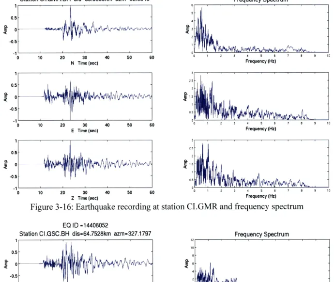
3-16 Earthquake recording at station CI.GMR and frequency spectrum ... 34

3-17 Earthquake recording at station CI.GSC and frequency spectrum ... 34

3-18 Earthquake recording at station CI.JVA and frequency spectrum ... 35

3-19 Earthquake recording at station CI.MCT and frequency spectrum ... 35 8

3-20 Filtered earthquake recording at station CI.DSC ... ... 36

3-21 Filtered earthquake recording at station CI.GMR ... ... 37

3-22 Filtered earthquake recording at station CI.GSC ... ... 37

3-23 Filtered earthquake recording at station CI.JVA ... 38

3-24 Filtered earthquake recording at station CI.MCT ... ... . 38

4-1 Station CRY with band pass filter applied ... 40

4-2 Station KNW with band pass filter applied ... 40

4-3 Station RDM with band pass filter applied ... ... 41

4-4 Station DGR with band pass filter applied ... ... 41

4-5 Station JCS with band pass filter applied ... ... ... 42

4-6 Best solution beach ball representation for earthquake 9718013 using 5 stations ... 43

4-7 Histograms of the best 200 solutions for earthquake 9718013 using 5 stations ... 45

4-8 Earthquake and 3 recording stations ... ... 46

4-9 Station KNW with band pass filter applied ... ... 46

4-10 Station RDM with band pass filter applied ... 47

4-11 Station DGR with band pass filter applied ... 47

4-12 Best solution beach ball representation for earthquake 9718013 using 3 stations ... 48

4-13 Histograms of the best 200 solutions for earthquake 9718013 using 3 stations ... 49

4-14 Station DSC with band pass filter applied ... ... 50

4-15 Station GMR with band pass filter applied ... ... 51

4-16 Station GSC with band pass filter applied ... ... 51

4-17 Station JVA with band pass filter applied ... ... 52

4-18 Station MCT with band pass filter applied ... 52

4-19 Best solution beach ball representation for earthquake 14408052 using 5 stations ... 53 9

4-20 Histograms of the best 200 solutions for earthquake 14408052 using 5 stations ... 55

4-21 Earthquake and 2 recording stations ... ... 56

4-22 Station DSC with band pass filter applied ... ... 56

4-23 Station GMR with band pass filter applied ... ... 57

4-24 Best solution beach ball representation for earthquake 14408052 using 2 stations ... 58

4-25 Histograms of the best 200 solutions for earthquake 14408052 using 2 stations ... 59

A-1 Input file for the discrete wavenumber code ... 62

List of Tables

3-1 Source location parameters for the two earthquakes ... 25

3-2 Mojave velocity model and quality factor ... ... 26

3-3 Southern California standard velocity model and quality factor . ... 26

3-4 List of stations used for event 9718013 ... .... 27

3-5 List of stations used for event 14408052 ... 27

4-1 Best 10 solutions in descending order for event 9718013 using 5 stations ... 44

4-2 Best 10 solutions in descending order for event 9718013 using 3 stations ... 48

4-3 Best 10 solutions in descending order for event 14408052 using 5 stations ... 54

Chapter 1

Introduction

1.1

Introduction

The objective of this thesis is to determine the focal mechanisms and depths of earthquakes by using full waveform synthetic seismograms. Studying earthquakes and determining their focal mechanisms is an active field of research in seismology. Many seismologists are determining focal mechanisms of earthquakes using various methods including the matching of full waveform seismograms. This research has different applications depending on the area or purpose for which these seismic event are studied. In earthquake-prone regions, such as Southern California where earthquakes are a great hazard, the focal mechanisms of seismic events are studied to better understand the stress and strain regime and earthquake hazard (Shen et al., 2007). In other regions, such as oil and gas fields, earthquakes are triggered by fluid injection and hydrocarbon extraction (Sarkar, 2008; Sze

et al., 2005). Monitoring these earthquakes helps to better characterize reservoirs and also helps to

determine where to produce or inject within a given hydrocarbon field (Maxwell, 2007).

Historically, studies of earthquake source mechanism have used short period body wave amplitude and polarity data. The most frequently used method is by studying the initial motion polarity of both primary (P) and secondary (S) waves from seismic recordings of many stations in order to draw the "beach ball" solution, which represents the focal mechanism of the earthquake (Nakamura, 2002). This method can be extended to include the amplitude data of P, SH, and SV with the polarity of the primary wave (Nakamura et al., 1999). Other approaches cross correlate the primary

waveforms to determine the focal mechanisms of earthquakes (Hansen et al., 2006). Another method that is used to determine the focal mechanism of earthquakes in Southern California involves using synthetic seismograms with relatively long periods to invert for the moment tensor (Qinya, 2006; Dreger, 2003).

The synthetic seismogram is the convolution of the source time function, Green's function weighted by the moment tensor components, and the instrument response. The source time function is assumed to be known and Green's function is calculated using information about the earthquake hypocenter, the seismic recording station location, and the velocity model of the subsurface. The instrument response can be found in the manual or by contacting the manufacturer of the instrument. The moment tensor is inverted for from the observed seismogram, Green's function, and the instrument response to find the focal mechanism of a given earthquake (Stein and Wysession, 2003).

One shortcoming of the currently used moment tensor inversion method is that only long periods or relatively low frequencies are used in the inversion. This is not adequate when we want to study the focal mechanism of relatively small magnitude earthquakes, which typically have higher frequencies. One of the problems of studying first motion polarities of primary and secondary waves is that it requires a large number of receivers in order to roughly draw the "beach ball" for the earthquake in question, and even if we had many stations, there will always be a large amount of uncertainty in where to draw the fault planes on the "beach ball". In principle, this shortcoming can be accounted for if we had a very large number of recording stations, which is not the case in reality.

In this thesis, I use synthetic seismograms and a grid search approach to find the best fit of the full waveforms in order to determine the source mechanism using short period data from a relatively few stations. In my approach, I generate full waveform synthetic seismograms and perform a grid

search to find the best combination of depth, strike, dip, and rake that will result in the synthetic seismogram with the best fit to the original observed seismogram. In order to do this, we have to know the velocity model of the subsurface and the epicenter of the earthquake of interest.

1.2

Thesis contents

The theoretical-numerical approach behind the full waveform modeling method is discussed in chapter two including an explanation of our grid search code that is used to find the best focal mechanism solution. Information about the earthquakes and the stations used to find their focal mechanism along with the Mojave and SoCal velocity models are included in chapter three. Results of this study and the discussion section are found in chapter four followed by conclusions in chapter five.

Chapter 2

Theoretical-Numerical Approach

2.1

Waveform modeling

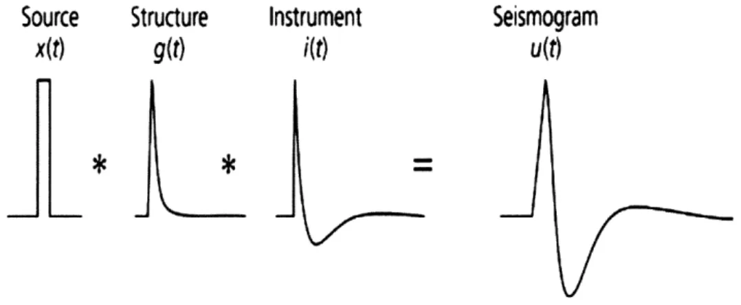
Looking at P-wave first motions is in many cases inadequate to determine the focal mechanisms of earthquakes. Therefore, considering the full waveform solution is essential in understanding and analyzing earthquakes (Stein and Wysession, 2003). The seismic signal that travels from the source within the earth to a receiver can be modeled in a simple diagram as seen in Figure 2-1.

Figure 2-1: System diagram of a seismogram (Scherbaum, 1994)

The seismic source generates the signal, which travels through the earth and is influenced by the response of the instrument that records the seismic signal. Therefore, the resulting seismogram u (t) can be written as in equation (1) and is shown in Figure 2-2.

u(t)=x(t)*e(t) *q(t) *i(t)

₍₁₎

e (t) is the elastic effect of the earth structure

q(t) is the anelastic effect of the earth structure i(t) is the instrument response of the seismometer

e(t) and q(t) are convolved to form Green's function g(t)

Source

Structure

Instrument

Seismogram

x(t)

g(t)

i(t)

U(t)

Figure 2-2: Seismogram as the convolution of the source, structure, and instrument signal

(Stein and Wysession, 2003)

Convolution in the time domain is equivalent to multiplication in the frequency domain. So we apply the Fourier transform to equation 1 and rewrite it in the form:

U (w)= X () E (w) Q(o) I(co) (2)

We will discuss each of these factors in the following sections to have a deeper understanding of the different components that make up a seismogram. There is one more component that affects a seismogram and that is noise. There are many known techniques in seismology to attenuate noise such as filtering, stacking and many others (Pujol, 2003; Kennett, 2001). We will not consider noise in this study because we will choose events with high signal to noise ratio and thus we can neglect the effect of noise.

2.2

The Source time function

The source time function denoted by x(t) in equation (1) is the earthquake's source signal that is produced by the rupture of the fault. It is dependent on the derivative of the history of slip on the fault. To better understand this concept, try to think of an earthquake that results from a short fault that slips instantaneously. The seismic moment function of this earthquake is a step function. The derivative of this step function, which is a delta function, is the source time function for this particular earthquake. Relatively small earthquakes are considered to occur along short faults, which can be treated as a single point source. Displacements along these faults are approximated as a smooth ramp function and that is what we will assume for the source time function in this study (Clinton, 2004). Larger earthquakes occur along longer faults and thus have a more complicated source time functions.

2.3

Green's function

The two terms e(t) and q(t) in equation (1) represent the elastic and anelastic effect of the

earth's structure respectively. The elastic term e(t) describes the wave propagation in the perfectly

elastic medium. It also describes the reflections and refractions at the different boundaries. The other term, namely, q(t) describes the attenuation of the seismic waves. This happens when part of the mechanical energy of the seismic waves is lost to the medium by converting to heat during

propagation. This attenuation can be described as a function of time (t) and angular frequency (ow) as

follows:

f(t,w)

Aeit

₍₃₎

The term Q in the equation above is the quality factor and it quantifies the amplitude decay

with time. Few important points to observe from equation (3) is that generally waves with higher frequency get attenuated faster than waves with lower frequency. We also note that the larger the

quality factor (Q), the slower the decay, and thus the less the attenuation. The values of (Q) for primary and shear waves are smaller for sediments and the waves get attenuated more in such mediums (Stein and Wysession, 2003). I want to point out here that the quality factor affect on our seismograms is negligible at the frequency ranges we will be working with, that is, 0.1 to 2.0 Hz, and the relatively short distances between the source and stations.

The elastic and anelastic terms e(t) and q(t), respectively can be convolved to get the Green's function in time domain g(t) as seen in equation (4), or in frequency domain as seen in equation (5):

g(t) =e(t)*q(t) (4)

G (w) = E (wo)

Q

Green's function is the signal that would arrive to the seismometer if the source were a point source (e.g. explosion) and the source time function was a delta function. Green's function can be expressed in the Cartesian coordinate system as a double integral over frequency and horizontal wavenumber for elastic layered medium with the origin of the coordinate system at the source location (Bouchon, 2003):

(x,y,z;o)) = iVl(e) e-iViz e-ikx -ikydkxdk, (6) with

2

v, 2 y- , Im(v)<0 (7)

where: is the displacement potential

w is the angular frequency

a is the P wave velocity

V, is the volume change at the source (Note: V,= 0 for an earthquake)

The integral in equation (6) can be discretized due to the interference of the waves and expressed as in equation (8) (Bouchon, 1981). This equation describes both the geometrical spreading of the wave and the attenuation. The reflectivity and transmissivity matrices of the layered medium are calculated for each wavenumber.

a(r,z;)= - E - Jo(knr)ei " (8)

L= V

with

k, =2nr/L; v = k -- k, (9)

where: 0a is the displacement potential

(0

a

w is the angular frequency

r is the distance between the source and the observation point z is the depth

k is the wavenumber

L is source array spacing

Jo is the zero order Bessel function

e_n is Neumann's factor and it is defined as

e,=2 ifn d 0

2.4

Instrument response

One of the factors that determine a seismogram is the instrument response i (t) as can be seen from equation (1). This will of course differ depending on the type of seismometer used. The instrument response is given by the manufacturer. The response of a seismometer changes with frequency and thus we have to account for that difference when trying to determine the focal mechanism of an earthquake. If the instrument response is flat at the frequency band we are interested in, then we can ignore the instrument response because it will have a small affect on the shape of the seismogram. Broadband seismograms have a flat response through most frequencies (Havskov and Alguacil, 2004). The seismic recording stations used in this study are all STS-2 broadband stations with flat instrument response at the frequency band we are interested in, namely, from 0.1 to 2.0 Hz as

can be seen in Figure 2-3 (Southern California Earthquake Data Center). Therefore, we will ignore

their responses. Figure 2-3 shows the frequency responses of broadband seismometers.

(F

Velocity Response vs. Frequency (Southern California Seismic Network)

-. I*

/ /

'-/

° -"----

r'"

2.5

Full waveform synthetic seismograms

The full waveform synthetic seismograms seen in this thesis will be generated using a modified version of a discrete wavenumber code written originally by Michel Bouchon as part of his MIT Ph.D. thesis (Bouchon, 1976). The code is based on a discrete wavenumber representation of elastic waves. The user specifies some parameters of the earthquake, the location of the stations, and the velocity model of the medium. The code calculates the moment tensor and weights it with Green's function, then convolves it with the source time function to produce the synthetic seismogram. Please refer to appendix (A) for more details about executing the code and the input and output files.

2.6 Matlab grid search code for source parameters

We developed a Matlab code version of the discrete wavenumber code with the improvement of optimizing the code so that it will perform a grid search through all the combinations of depths, strikes, dips, and rakes in a reasonable time frame on the order of a few minutes to a few hours depending on how small we choose our search intervals. The code was modified to calculate Green's functions for five different depths with the midpoint being the initial estimate of the depth and 2 km above and below that depth with a 1 km grid interval. This operation is performed only once since Green's function depends only on the source and receiver locations and the velocity structure, which is constant for a single pair of earthquake and seismic recording station. The code then calculates the moment tensor, which is dependant on the focal mechanism of the earthquake. This is done for different combinations of strikes, dips, and rakes. We specify the search interval to be 100 and start

from 0O to 3500, 00 to 900, and -900 to 900 for the strike, dip, and rake, respectively. This means that

we have 36 x 10 x 19 = 6840 different combinations of strikes, dips, and rakes. Green's functions are

source time function to produce synthetic seismograms. This whole operation results in 36 x 10 x 19 x

5 = 34200 different synthetic seismograms for one seismic station. A Butterworth band pass filter with

frequency band of 0.1 to 2.0 Hz is applied to these seismograms and they are cross-correlated and

normalized with the observed seismogram. L2 norm is added to the code in order to consider the

amplitude match when performing the cross correlation and not only the phases of the waveforms. This is done independently for each component of each seismic station to allow for differences that arise from anisotropy and heterogeneity in the subsurface of the earth (Sileny and Vavrycuk, 2002).

The code performs a joint grid search by considering a group of stations and not only one station, and finds the best fit between the filtered observed and filtered synthetic seismograms that suit all three components of all the seismic stations used to study a single earthquake. The best fit is calculated using the following objective function (Li et al., 2009):

N 3

maximize (J(strike, dip, rake, depth))= A, max(d v )- A2 d v ]

n=1 j=1 2

The objective function (J) seen above consists of A1 through A2, which are predetermined

weights for each of the two terms. The first term evaluates the maximum cross correlation between the

normalized (relative to maximum amplitude) observed data (d]) and normalized synthetic waveforms

(v'), where n denotes the station number, 0 denotes cross correlation, and j denotes the component

(north, south, vertical). The second term evaluates L2 norm, the direct difference between the synthetic

and observed seismograms.

The corresponding strike, dip, and rake is the focal mechanism of the earthquake we are investigating, and the depth determines the hypocenter of the earthquake since we assume that the epicenter is known.

Chapter 3

Earthquake Data

3.1

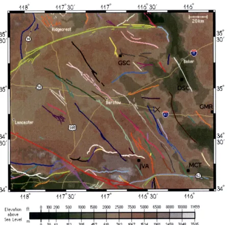
Earthquakes

We test out method using seismograms from two earthquakes in Southern California. The epicenters of the events and the stations used to invert for the focal mechanism are shown in Figures 3-1 and 3-3. Maps with the major faults in the area of interest are shown in Figure 3-2 and 3-3 and a table with the source location parameters is shown in Table 3-1.

350 N

34" N

33°N

Stations used for event 9718013 (5 stations)

4000 3500 3000 2500 2000 1500 1000 500 1321 W 117" W 116 ° _{W 115" W}

118- 17130' 1147 11630' 116 115 30'

Elevation ft 0 100 200 500 1000 1500 2000 2500 3500 5000 6500 8000 10000 12000

above

Sea Level m

0 30 61 152 305 457 610 762 1067 1524 1381 2438 3048 3657

Figure 3-2: Earthquake 9718013 (cross sign) and 5 recording stations (black squares)

(Southern California Earthquake Data Center)

Stations used for event 14408052 (5 stations)

381

120°W 1180W 116 W 114' W 112

Figure 3-3: Earthquake 14408052 (red star) and 5 recording stations (yellow circles)

5" 30' 350 34o lie 117°30' 117" 11 6 30' 116° Elevation ft 0 100 200 500 1000 1500 2000 2500 3500 5000 6500 8000 10000 11499 above Sea Level m 0 30 61 152 305 457 610 762 1067 1524 1381 2438 3048 3505

Figure 3-4: Earthquake 14408052 (cross sign) and 5 recording stations

(Southern California Earthquake Data Center)

(black squares) Earthquake ID Latitude 9718013 33.508 14408052 34.813 Table 3-1: Source Longitude -116.514 -116.419 location parameters Magnitude 5.02 5.06

for the two

Date Origin time

31 Oct 2001 07:56:16.63

6 Dec 2008 04:18:42.85

earthquakes (SCEC)

3.2

Velocity models

The Southern California Earthquake Data Center (SCEC) released version 4, which is a new 3-D velocity model of Southern California, in 2005. The Mojave and SoCal velocity models seen below are good approximations but are not exactly identical to the most recent SCEC velocity model. This is expected because the SCEC velocity model is too smooth to generate any meaningful seismograms using the discrete wavenumber (DWN) code. Another point to clarify here is that the velocity model varies from one location to the other. In other words, the layers are not horizontal. This presents a

I

problem because the code used here only deals with horizontal layers. Therefore, the SoCal and Mojave velocity models seen below are used because they overcome the issues mentioned above and

at the same time are good approximations to the SCEC velocity model.

3.2.1

Mojave velocity model

Thickness (km) P (km/s) S (km/s) Density (g/cm3) Q Qs

2.5 5 2.6 2.4 70 40

3 5.5 3.45 2.4 100 50

22.5 6.3 3.6 2.67 150 75

Half space 7.85 4.4 3.42 200 100

Table 3-2: Mojave velocity model (Jones and Helmberger, 1998), (Erickson et al., 2004)

and quality factor

3.2.2

SoCal velocity model

Thickness (km) P (km/s) S (km/s) Density (g/cm3) Q Qs

5.5 5.5 3.18 2.4 70 40

10.5 6.3 3.64 2.67 100 50

16 6.7 3.87 2.8 150 75

Half space 7.85 4.5 3.42 200 100

Table 3-3: Southern California standard velocity model (Dreger 1993), and quality factor (Erickson et al., 2004)

and Helmberger,

3.3

Seismic Recording Stations

The five stations used to find the focal mechanism and depth of earthquakes 9718013 and 14408052 are listed in Tables 3-4 and 3-5, respectively. These stations were chosen from a larger set of stations available in Southern California so that we will have relatively good azimuth coverage. Then the method is repeated using a subset of these stations with relatively poor azimuth coverage.

3.3.1

Stations used for event 9718013

Station Latitude Longitude Distance (km) Azimuth

AZ.KNW 33.7141 -116.7119 29.34 321.40

CI.JCS 33.0859 -116.5959 47.54 189.23

AZ.CRY 33.5654 -116.7373 21.65 287.20

CI.DGR 33.6500 -117.0094 48.54 289.12

AZ.RDM 33.6300 -116.8478 33.77 293.77

Table 3-4: List of seismic stations used for event 9718013

3.3.2

Stations used for event 14408052

Station Latitude Longitude Distance (km) Azimuth

CI.DSC 35.1425 -116.1039 46.54 37.98

CI.GMR 34.7845 -115.6599 69.38 92.39

CI.GSC 35.3017 -116.8057 64.75 327.17

CI.JVA 34.3662 -116.6126 52.74 199.69

CI.MCT 34.2264 -116.0407 73.85 151.90

Table 3-5: List of seismic stations used for event 14408052

Seismograms

3.4.1

Raw seismograms of event 9718013

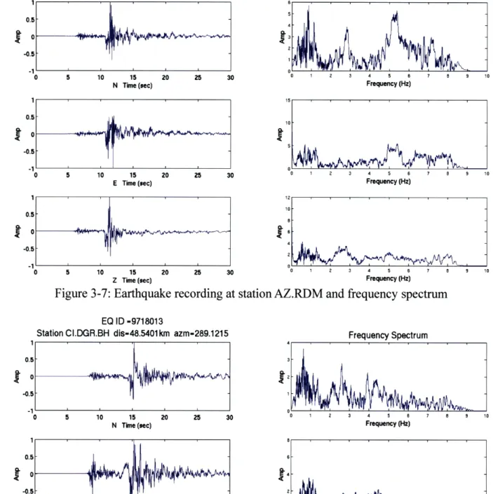
In Figures 3-5 to 3-9, we show the three components (N, E, Z) of each of the five stations

along with their frequency spectra. The sampling interval of the original seismograms is 0.05 seconds,

and the sampling frequency is 1/0.05 seconds = 20 Hz. The following seismograms have a Nyquist

frequency of 10 Hz.

EQ ID -9718013

Station AZ.CRY.BH dis-21.6583km azm-287.2009

N Time(sec) 0 5 10 15 20 25 3 E Tie (sec) , , , Frequency Spectrum Frequency (Hz) Frequency (Hz) 0 5 10 15 Z Time (sec) 20 25 30 Frequency (Hz)

Figure 3-5: Earthquake recording at station AZ.CRY and frequency spectrum

EQ ID -9718013

Station AZ.KNW.BH dis-29.3438km azm-321.4061

N Time (sec) Frequency Spectrum 5 4 3 0 1 2 3 4 5 6 7 8 9 Frequency (Hz) 0.5 0 -0.5 -1 0 5 10 15 E Time (sec) 20 25 30 0.5 -0.5 0 5 10 15 20 25 30 Z Time (sec)

Figure 3-6: Earthquake recording at station

0 1 2 3 4 5 6

Frequency (Hz)

7 8 9 10

AZ.KNW and frequency spectrum Frequency (Hz)

EQ ID -9718013

Station AZ.RDM.BH dis-33.771km azm-293.7767 Frequency Spectrum

0.5 -0.5 -1 ' 0 5 10 15 20 25 3( N Time (sec) i, 5 10 15 20 25 30 E Time (sec) 0 5 10 15 20 25 30 Z Time (sec) 15 10 0 1 2 3 4 5 6 7 a 9 10 Frequency (Hz) 12 0 0 1 2 3 4 5 6 7 a 9 10 Frequency (Hz)

Figure 3-7: Earthquake recording at station AZ.RDM and frequency spectrum EQ ID -9718013

Station CI.DGR.BH dis-48.5401km azm-289.1215 _{Frequency Spectrum}

15 20 25 30 0 1 2 3 4 5 6 7 e 9 10

N Time (sec) Frequency (Hz)

4-0 1 2 3 4 5 6 7 6 9 1

Frequency (Hz)

10

5 10 15 20 25 30 0 1 2 3 4 6 7 0 10

Z Time (sec) Frequency (Hz)

Figure 3-8: Earthquake recording at station CI.DGR and frequency spectrum 0.5

-0.5

Frequency (Hz)

EQ ID -9718013

Station CI.JCS.BH dis-47.5486km azm-189.2344 .5 .5 -1I I i I 0 5 10 15 20 25 31 N Time (sec) .5 -.5 .5 i i 0. -0. 0. -0. 5 10 15 E Time (sec) 20 25 30 Frequency Spectrum Frequency (Hz) Frequency (Hz) 0 5 10 15 20 25 30 0 1 2 3 4 5 6 7 a 9 12

Z Time (sec) Frequency (Hz)

Figure 3-9: Earthquake recording at station CI.JCS and frequency spectrum

3.4.2

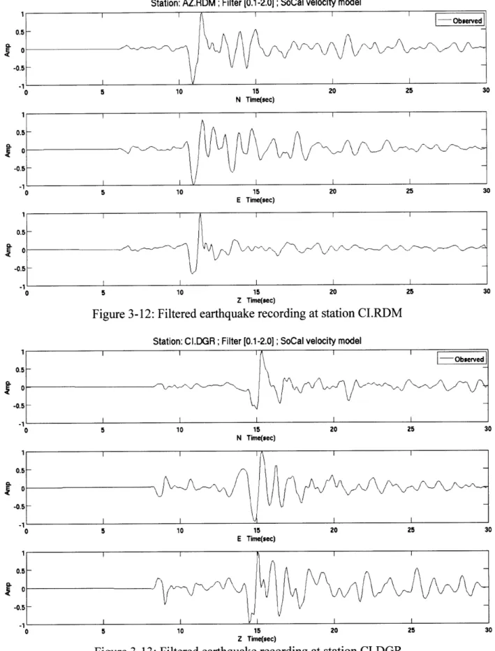
Filtered seismograms of event 9718013

The filtered observed seismograms are shown in Figures 3-10 to 3-14. At most stations, the amplitude spectra have high values at frequencies lower than 2.0 Hz. The observed seismograms are re-sampled to 20/256 = 0.0781 seconds to match the sampling interval of the synthetic seismograms of event 9718013, which will be shown in the results and discussion section in chapter four. We didn't do the opposite, namely, calculate the synthetic seismograms every 0.05 seconds because it slows down the calculation time significantly. A Butterworth band pass filter with frequency band of 0.1 to 2.0 Hz is applied to these re-sampled observed seismograms and the resultant five seismograms are shown below.

Station: AZ.CRY; Filter [0.1-2.0]; SoCal velocity model

5 10 15 20 25

N Time(sec)

E Time(sec)

Z Time(sec)

Figure 3-10: Filtered earthquake recording at station AZ.CRY Station: AZ.KNW; Filter [0.1-2.0]; SoCal velocity model

-Observed 5 10 15 20 25 3 N Time(sec) 0 5 10 15 20 25 E Time(sec) -1 0 5 10 15 20 25 Z Time(sec)

Figure 3-11: Filtered earthquake recording at station AZ.KNW

0.5 0--0.5 -1 0 I I I I ' - I

Station: AZ.RDM; Filter [0.1-2.01; SoCal velocity model

N Time(sec)

E Time(sec)

Z Time(sec)

Figure 3-12: Filtered earthquake recording at station CI.RDM Station: CI.DGR ; Filter [0.1-2.01 ; SoCal velocity model

N Time(sec)

E Time(sec)

0 5 10 15 20 25 30

Z Time(sec)

Station: CI.JCS; Filter [0.1-2.01; SoCal velocity model

N Time(ec)

E Time(.ec)

0 5 10 15 20 25 30

Z Tnie(ec)

Figure 3-14: Filtered earthquake recording at station CI.JCS

3.4.3

Raw seismograms of event 14408052

In Figures 3-15 to 3-19, we show the three components (N, E, Z) of motion recorded at each of the five stations along with the frequency spectra. The sampling interval of the original seismograms is

0.05 seconds, and the sampling frequency is 1/0.05 seconds = 20 Hz. The following seismograms have

a Nyquist frequency of 10 Hz.

EQ ID -14408052

Station CI.DSC.BH dis-46.5482km azm-37.9822 Frequency Spectrum

-0.5 2

-1 0

0 10 20 30 40 50 60 1 2 3 4 s 6 7 e s o

N Time (eec) Frequency (Hz)

0.5 6

-0.5

0 10 20 30 40 50 60 o 1 4 0 6 7 e S 10

E Time (sec) Frequency (Hz)

0.50

-0.5-0 10 20 30 40 50 60 0 1 2 3 4 5 i 7 9 10

Z Time (ec) Frequency (H)

EQ I D -14408052

Station CI.GMR.BH dis-69.3809km azm-92.3949

0 10 20 30 N Time (sec) 40 50 Frequency Spectrum 6 5 44 5 6 3 2 0123456781E _{Frequency (Hz)} 5 5 1 .5 0 1 2 3 4 5 6 Frequency (Hz) 7 6 9 10 10 20 30 40 50 60 .. . .

Z Time (sec) Frequency (Hz)

Figure 3-16: Earthquake recording at station CI.GMR and frequency spectrum

EQ ID =14408052

Station CI.GSC.BH dis-64.7528km azm-327.1797 1 ).5 0 1.5 -1 0 10 20 30 40 50 6( N Time (sec) 0 10 20 30 E Time (sec) 40 50 60 Frequency Spectrum 10 8 o 0 1 2 3 4 5 6 7 0 9 1 Frequency (Hz) 20 15 in 0 1 2 3 4 5 6 Frequency (Hz) 7 a 9 10 0.5 0 -0.5 -1 - 0 0 10 20 30 40 50 60 Z Time (sec)

Figure 3-17: Earthquake recording at station CI.GSC

2 3 4 5 6

Frequency (Hz)

7 8 9 10

and frequency spectrum E Time (sec)

0.5

-0.5 -1

EQ ID -14408052

Station CI.JVA.BH dis-52.7478km azm-199.6934

N Time (sec) E Time (sec) Frequency Spectrum 6 4 0 0 1 2 3 4 5 6 7 8 9 1 Frequency (Hz) 15 0 1 2 3 4 5 6 Frequency (Hz) 30 Z Time (sec) 2 3 4 5 6 7 10 Frequency (Hz) Figure 3-18: Earthquake recording at station CI.JVA and frequency spectrum

EQ ID -14408052

Station CI.MCT.BH dis-73.8569km azm-151.9083 5 0 5 40 50 Frequency Spectrum 0 1 2 3 4 5 6 Frequency (Hz) 7 8 9 10 Frequency (Hz) 10 20 30 40 50 60 Z Time (sec)

Figure 3-19: Earthquake recording at

0 1 2 3 4 5 6 7 6

Frequency (Hz)

station CI.MCT and frequency spectrum

7 6 9 10

0 10 20 30 N Time (sec)

3.4.4

Filtered seismograms of event 14408052

The filtered observed seismograms are shown in Figures 3-20 to 3-24. At most stations, the amplitude spectrum has high values at frequencies lower than 2.0 Hz. The observed seismograms are

re-sampled to 23/256 = 0.0703 seconds to match the sampling interval of the synthetic seismograms of

event 14408052, which will be shown in the results and discussion section in chapter four. We didn't do the opposite, namely, calculate the synthetic seismograms every 0.05 seconds because it slows down the calculation time significantly. A Butterworth band pass filter with frequency band of 0.1 to 2.0 Hz is applied to these re-sampled observed seismograms and the resultant five seismograms are shown below.

Station: CI.DSC ; Filter [0.1-2.0] ; Mojave velocity model

0Observed -0.5 1I I I I I I I 0 5 10 15 20 25 30 35 40 45 50 N Time(sec) 1 I I 1 I I 1 I I I 0.5E 0 5 10 15 20 25 30 35 40 45 50 E Time(sec) 0 5 10 15 20 25 30 35 40 45 50 Z Time(sec)

Station: CI.GMR; Filter [0.1-2.01 ; Mojave velocity model 1 0.5-0 -0.5--1 0 30 35 40 45 ' E Time(sec) Z Time(sec)

Figure 3-21: Filtered earthquake recording at station CI.GMR Station: CI.GSC ; Filter [0.1-2.0]; Mojave velocity model

N Time(sec)

10 15 20 25 30 35 40 45 50

E Time(sec)

10 15 20 25 30 35 40

Z Time(sec)

Figure 3-22: Filtered earthquake recording at station CI.GSC

10 15 20 25 N Time(sec) -Observed 5 0.5 00.5 --1 0 1- 0.5- 0- -0.5--10₀ 45 50 -I I I

Station: CI.JVA; Filter [0.1-2.0]; Mojave velocity model 5 10 15 20 25 30 35 40 45 N Time(sec) 5 10 15 20 25 30 35 40 45 51 E Time(sec) 0

1

0

Figure 3-24: Filtered earthquake recording at station CI.MCT

45 50

I II I I I

5 10 15 20 25 30 35 40

Z Time(sec)

Figure 3-23: Filtered earthquake recording at station CI.JVA Station: CI.MCT; Filter [0.1-2.0] ; Mojave velocity model

SI I I I I I I -0.5 -1 0 I

f

Chapter 4

Results and Discussion

4.1

Earthquake ID 9718013

4.1.1

Joint modeling using 5 stations

We use the joint grid search code to get the best combination of depth, strike, dip, and rake that results in the best fit between the filtered synthetic and filtered observed seismograms for all three components of motion and for all the five stations. The best fit is determined using cross correlation

and L2 norm, which are built-in Matlab functions and this is explained in further detail in section 2.6.

The time duration used in the matching of the synthetic and observed seismograms for stations CRY, KNW, RDM, DGR, JCS are 13, 14, 15, 18, and 18 seconds, respectively. The length of the synthetic seismogram is determined by observing the initial match between the synthetic and observed seismograms, then determining where the fit of the synthetic seismogram starts to deteriorate. We choose different time duration for each station depending on our observations of the match between the synthetic and observed seismogram.

I will use the Southern California standard velocity model (SoCal), which is defined earlier in this thesis for this earthquake. I will show plots of the best-fit solution of the filtered synthetic seismograms overlaying the filtered original seismogram for each component, that is, the north-south, east-west, and vertical components, and I will do so for each of the five stations.

Station: AZ.CRY; Filter [0.1-2.0]; SoCal velocity model Observed .5 Synthetic II I I I I I II 10 N Time(sec) 12 14 16 18 20 ) 2 4 6 8 10 12 14 16 18 20 E Time(sec) 10 Z Time(sec) 12 14 16 18

Figure 4-1: Station CRY with band pass filter applied Station: AZ.KNW; Filter [0.1-2.0]; SoCal velocity model

N Time(sec) E Time(sec) 1 I I I I I I I

5-0

j

Figure 4-2: Station KNW with band pass filter applied

Station: AZ.RDM; Filter [0.1-2.0]; SoCal velocity model 1 I I I I I I iI Observed .5- -- Synthetic .5 8 10 N Time(sec) 12 14 16 E Time(sec) N Time(sec) I I-I I 5 5 -1 1 1 1 1 I 10 E Time(sec) 16 18 20 12 14 16 18 20 0 -0 18 20 4 6 8 10 12 14 Z Time(sec)

Figure 4-3: Station RDM with band pass filter applied Station: CI.DGR; Filter [0.1-2.0]; SoCal velocity model

0.! -0. 0. -0. 0 1 5- 0-5 1 0 4 6 8 10 12 14 Z Time(sec)

Figure 4-4: Station DGR with band pass filter applied

16 18 20

-0.5

-1

Station: CI.JCS; Filter [0.1-2.01; SoCal velocity model SObserved 0.5 - Synthetic 0 2 4 6 8 10 12 14 16 18 20 N Time(sec) 0.5 -0.5 -0.1 I I i I I III I I -1 0 _{0 2} 2 ₄ 4 ₆ 6 8 8 10 10 12 12 14 14 16 16 18 18 2020 Z Time(sec)

Figure 4-5: Station JCS with band pass filter applied

It is obvious from the above five Figures that our joint grid search code did a very good job in finding a solution especially if we considered that the solution managed to fit all three components of motion recorded at each station and did so for all five stations, which gives us a great amount of confidence in the solution. The parameters of this best solution puts the depth of the earthquake at 15 km with a strike, dip, and rake of 300, 60, and -170, respectively. The best ten solutions (Table 4-1) all give similar focal mechanisms. This is all done with a filtering frequency band of 0.1 to 2.0 Hz. The results can be compared to Southern California Earthquake Data Center's moment tensor solution, which puts the earthquake at a depth of 8 km with a strike, dip, and rake of 318, 33, and -180, respectively. The Southern California Earthquake Data Center puts the earthquake at a depth of 15.22 km, which is consistent with our results (Southern California Earthquake Data Center). The focal mechanism as we can see comparing the two sets of solutions are reasonably identical except for the dip. The dip of strike-slip faults in Southern California are closer to vertical and a dip of 60 is more

reasonable for faults in Southern California than a much shallower dip of 33 (Tok6z, M. Nafi, personal communication, March 2009).

The "beach ball" solution representing this focal mechanism is shown below in Figure 4-6. Looking at it, it is clear that this is a right lateral strike slip fault. The strike of the fault is consistent with the northwest, southeast orientation of the faults in the region as seen in Figure 3-2. It is also worth noting that stations that are located to the west or east of the earthquake are expected to have a more pronounced P-wave first arrival in the east-west component compared to the north-south

component. That explains the relatively small amplitude of the P-wave first arrival in the north-south component of station CRY compared to the east-west component as seen in Figure 4-1. Similarly, the amplitude of the P-wave first arrival in the north-south component is relatively large compared to the east-west component for station JCS, shown in Figure 4-5, because it lies almost directly to the south of the earthquake. The P-waves first arrivals are expected to be relatively weak in amplitude when the station's azimuth lies close to the nodal plane of the "beach ball" solution. This is due to the fact that the stress switches from compression, represented by an upward polarity for the P-wave first arrival, to dilation, represented by a downward polarity for the P-wave first arrival. This can be seen in all components of station RDM shown in Figure 4-3 because it has an azimuth of 293.70, which is close to the strike of the fault.

Strike - 300; Dipy 60 ;Rake --170

330 30 KNW RDM 300 60 DGR CRY 270 90 240 120 Z10 150 180 Jcs

Solution # Strike Dip Rake Depth (km) Goodness of fit 1 300 60 -170 15 37.89 2 300 60 -160 15 37.15 3 300 50 -170 15 37.00 4 300 50 -180 15 36.77 5 300 70 -160 15 36.64 6 300 50 170 15 36.29 7 300 50 -160 15 36.23 8 300 60 -180 15 36.19 9 310 50 160 15 36.09 10 310 50 170 15 35.86

Table 4-1: Best 10 solutions in descending order for event 9718013 using 5 stations

Histograms of strike, dip, rake, and depth of the best 200 solutions for event 9718013 using five stations are shown in Figure 4-7. Depth is the most constrained parameter because it has the smallest standard deviation percentage. Notice that the depth values do not look like a typical bell shaped curve because we choose the depth interval in the grid search to be constrained between 11 km and 15 km. If we had allowed the depth to have larger limits, we would expect the depth histogram to look more symmetric. Dip values are spread out over most possible values and have a relatively large standard deviation percentage compared to the other three parameters, which makes the dip the least constrained parameter. This could be due to the fact that all five recording stations used to model the focal mechanism of this earthquake are to the northwest and south of the earthquake's epicenter with no station coverage on the east as shown in Figure 3-1. The values of strike that represent the same nodal plane are taken to be the larger strike value. For example if the strike is 310, then it is represented on the histogram as 310. However, if the strike is 130, which is equivalent to a strike of 310, then the strike value is converted from 130 to 310 and represented as such in the histogram. Similarly, values of rake are converted to the larger positive equivalent to make it easier to see in the histogram. For example, if the rake is 170 then it is represented as 170. However, if the rake is -170,

then we add 360 to that to arrive to the equivalent positive rake of 190 and it is represented as such in the histogram.

Mean =302.55 % Standard deviation = 5.6524

100r-F--- , ---80 60 40I 20 100 150 Mean =187.55 200 250 300 350 Strike % Standard deviation = 13.1313

Mean =49.3 % Standard deviation = 36.9687

40 35-30 - 20-15 LL. 10-5r 0 0 10 20 30 40 50 60 70 80 90 Dip

Mean =14.68 % Standard deviation = 3.1856

40 140 35- 120 30 100 025 0 C 80 20 1560 ,, U. 40 10 5 20 0 0 0 50 100 150 200 250 300 350 11 12 13 14 15 16 Rake Depth (km)

Figure 4-7: Histograms of the best 200 solutions for earthquake 9718013 using 5 stations

We used five stations to find the focal mechanism of earthquake 9718013 and obtained a very good fit between the observed and synthetic seismograms. The fact that all the best ten solutions are consistent makes us confident in our results and in our full waveform modeling method.

4.1.2

Joint modeling using 3 stations

We will test our method using three stations with poor azimuth coverage, shown in Figure 4-8, and compare our results with the results we obtained using five stations.

Stations used for event 9718013 (3 stations) 35° N 4000 3500 3000 34° N 2500 2000 1500 33" N 1000 500 32' N0~ 1 , W 117° W 116° W 115°W

Figure 4-8: Earthquake (red star) and 3 recording stations (yellow circles)

Station: AZ.KNW; Filter [0.1-2.0] ; SoCal velocity model

N Time(sec)

E Time(sec)

0 2 4 6 8 10 12 14 16 18 20

Z Time(sec)

Station: AZ.RDM; Filter [0.1-2.0]; SoCal velocity model

E Time(sec)

Figure 4-10: Station RDM with band pass filter applied Station: CI.DGR ; Filter [0.1-2.0]; SoCal velocity model

N Time(sec)

E Time(sec)

0 2 4 6 8 10 12 14 16 18 20

Z Time(sec)

Once again our grid search found a very good match between the filtered observed and filtered synthetic seismograms for all three components of the three stations as shown in Figures 4-9 to 4-11. The ten best solutions are shown in Table 4-2 and they all show similar focal mechanisms. This gives us confidence in our modeling method. The focal mechanism here is similar to the one we got previously when we used five seismic stations. The depth is 14 km with a strike, dip, and rake of 300, 60, and -180, respectively. The "beach ball" solution is shown in Figure 4-12. This suggests that the fault is a right lateral strike slip fault.

RD D

Figure 4-12: Best solution beac

Strike - 300; Dip 60 ; Rake - -180

330 30 KNW GR 270 90 240 120 210 150 180

i ball representation for earthquake 9718013 using 3 stations

Solution # Strike Dip Rake Depth (km) Goodness of fit

1 300 60 -180 14 28.85 2 300 60 -170 15 28.62 3 300 70 -160 14 28.43 4 300 60 -170 14 28.41 5 300 50 170 14 28.28 6 310 60 160 14 28.24 7 300 50 -180 14 28.22 8 310 60 170 14 28.14 9 310 70 -180 14 28.13 10 300 50 -170 14 28.02

Table 4-2: Best 10 solutions in descending order for event 9718013 using 3 stations

We show the histograms of the best 200 solutions of strike, dip, rake, and depth for event 9718013 using three stations in Figure 4-13. The strike has the smallest standard deviation percentage

and thus is the most constrained parameter. The dip still has the largest standard deviation percentage and thus is again the least constrained parameter. The strike, rake, and depth are still relatively well constrained. Notice that we have converted the values of strike and rake exactly as we did in the previous example. For example, we added 360 to all negative values of rake to obtain the equivalent positive rake value so that it will be easier to draw the histogram.

% Standard deviation = 2.1979

150 200 250 300 350

Strike

Mean =55.05 % Standard deviation = 27.9166

100 80 60 40 20 0 0 0 10 20

Mean =190.8 % Standard deviation = 11.1008 Mean =13.975

40 r- --- 80 35 70 30 60} 025 050 C IC 20 40 15- 30H LL -10 20 0 50 100 150 200 250 300 350 11 12 Rake

Figure 4-13: Histograms of the best 200 solutions for earthqual

40 50 60 70 80 90 Dip % Standard deviation = 5.6228 , • , 13 14 15 16 Depth (km) ke 9718013 using 3 stations

4.2

Earthquake ID 14408052

4.2.1

Joint modeling using 5 stations

We will test our method with another earthquake in Southern California. We use the joint grid search code to get the best combination of depth, strike, dip, and rake that results in the best fit

Mean =304.3 I,, 80 60 40-LL 20 0 1 100

between the filtered synthetic and filtered observed seismograms for all three components and for all the five stations. The best fit is determined using cross correlation and L2 norm, which are built-in

Matlab functions. Further details on how the best fit is determined can be found in section 2.6. The time duration used in the matching of the synthetic and observed seismograms for stations DSC, GMR, GSC, JVA, MCT are 17, 22, 22, 18, and 20 seconds, respectively. I use the Mojave velocity model, which is defined earlier in this thesis, for this earthquake. In Figures 4-14 to 4-18, I show plots of the best-fit solution of the filtered synthetic seismogram overlaying the filtered original seismogram for each component, namely, the north-south, east-west, and vertical components, and I will do so for each of the five stations.

Station: CI.DSC; Filter [0.1-2.0]; Mojave velocity model

E Time(sec)

0 2 4 6 8 10 12 14 16

Z Time(sec)

Figure 4-14: Station DSC with band pass filter applied

Station: CI.GMR ; Filter [0.1-2.0] ; Mojave velocity model N Time(sec) -1I I I I I I 0 2 4 6 8 10 12 14 16 18 20 22 E Time(sec) 1 I I I I 0.5 0.5 --o1 1 I I I I I I I I 0 2 4 6 8 10 12 14 16 18 20 22 Z Time(sec)

Figure 4-15: Station GMR with band pass filter applied Station: CI.GSC; Filter [0.1-2.0] ; Mojave velocity model

-Observed 0.5 - Synthic 0.5 -0 2 4 6 8 10 12 14 16 18 20 22 N Time(sec) 0.5

-1

CL