Grazing and the vanishing complexity of plant association networks in grasslands

HAL Id: hal-03123198

https://hal.archives-ouvertes.fr/hal-03123198

HAL is a multi-disciplinary open access

archive for the deposit and dissemination of sci-entific research documents, whether they are pub-lished or not. The documents may come from teaching and research institutions in France or abroad, or from public or private research centers.

L’archive ouverte pluridisciplinaire HAL, est destinée au dépôt et à la diffusion de documents scientifiques de niveau recherche, publiés ou non, émanant des établissements d’enseignement et de recherche français ou étrangers, des laboratoires publics ou privés.

Grazing and the vanishing complexity of plant

association networks in grasslands

Alexandre Génin, Thierry Dutoit, Alain Danet, Alice Le Priol, Sonia Kéfi

To cite this version:

Alexandre Génin, Thierry Dutoit, Alain Danet, Alice Le Priol, Sonia Kéfi. Grazing and the vanish-ing complexity of plant association networks in grasslands. Oikos, Nordic Ecological Society, 2021, �10.1111/oik.07850�. �hal-03123198�

Grazing and the vanishing complexity of plant association networks in grasslands Alexandre Génin1 Thierry Dutoit2 Alain Danet1,3 Alice le Priol1 Sonia Kéfi1,4

1 ISEM, CNRS, Univ. Montpellier, IRD, EPHE, Montpellier, France

2 Avignon Université, Aix Marseille Univ, CNRS, IRD, IMBE, Avignon, France.

3 Centre d’Ecologie et des Sciences de la Conservation, CNRS, MNHN, Sorbonne Université, Paris, France. 4 Santa Fe Institute, 1399 Hyde Park Road, Santa Fe, NM 87501, USA

Abstract

Interactions are key drivers of the functioning and fate of plant communities. A traditional way to measure them is to use pairwise experiments, but such experiments do not scale up to species-rich communities. For those, using association networks based on spatial patterns may provide a more realistic approach. While this method has been successful in abiotically-stressed

environments (alpine and arid ecosystems), it is unclear how well it generalizes to other types of environments.

We help fill this knowledge gap by documenting how the structure of plant communities changes in a Mediterranean dry grassland grazed by sheep using plant spatial association networks. We investigated how the structure of these networks changed with grazing intensity to show the effect of biotic disturbance on community structure.

We found that these grazed grassland communities were mostly dominated by negative associations, suggesting a dominance of interference over facilitation regardless of the

disturbance level. The topology of the networks revealed that the number of associations were not evenly-distributed across species, but rather that a small subset of species established most negative associations under low grazing conditions. All these aspects of spatial organization vanished under high level of grazing as association networks became more similar to null expectations.

Our study shows that grazed herbaceous plant communities display a highly non-random organization that responds strongly to disturbance and can be measured through association networks. This approach thus appears insightful to test general hypotheses about plant communities, and in particular understand how anthropogenic perturbations affect the organization of ecological communities.

Keywords

Plant–plant interactions, Grazing, Association networks, Ecological Networks, Spatial patterns, Co-occurrence

Acknoweldgements

The authors warmly thank the staff from the Réserve Nationale des Coussouls de Crau for the numerous discussions and their help with logistics, with a specific thought to L. Tatin and A. Wolff. We also thank the members of the BioDICée team at ISEM along with J. Azuara and C. Kouchner for their help with field work, and D. Pavon (IMBE) for his help with plant

identification. AG would like thank T. Daufresne, S. Boudsocq and J. Delarivière from

Eco&Sols (INRA) for their help with soil processing, sampling and survey design. The study has been supported by the TRY initiative on plant traits (http://www.try-db.org), maintained by J. Kattge and G. Bönisch (Max Planck Institute for Biogeochemistry, Jena, Germany), and supported by DIVERSITAS/Future Earth and the German Centre for Integrative Biodiv. Research (iDiv) Halle-Jena-Leipzig.

Author contributions

AG led conceptual framing, field work, data analyses and manuscript writing. AD and AlP helped with conceptual framing and field work. SK and TD provided significant support and advice all along the project. All authors contributed substantially to the manuscript writing and editing.

Grazing and the vanishing complexity of plant association networks in grasslands

Abstract

Interactions are key drivers of the functioning and fate of plant communities. A traditional way to measure them is to use pairwise experiments, but such experiments do not scale up to species-rich communities. For those, using association networks based on spatial patterns may provide a more realistic approach. While this method has been successful in abiotically-stressed environments (alpine and arid ecosystems), it is unclear how well it generalizes to other types of environments.

We help fill this knowledge gap by documenting how the structure of plant communities changes in a Mediterranean dry grassland grazed by sheep using plant spatial association networks. We investigated how the structure of these networks changed with grazing intensity to show the effect of biotic

disturbance on community structure.

We found that these grazed grassland communities were mostly dominated by negative associations, suggesting a dominance of interference over facilitation regardless of the disturbance level. The topology of the networks revealed that the number of associations were not evenly-distributed across species, but rather that a small subset of species established most negative associations under low grazing conditions. All these aspects of spatial organization vanished under high level of grazing as association networks became more similar to null expectations.

Our study shows that grazed herbaceous plant communities display a highly non-random organization that responds strongly to disturbance and can be measured through association networks. This approach thus appears insightful to test general hypotheses about plant communities, and in particular understand how anthropogenic perturbations affect the organization of ecological communities.

Introduction

1 2

Ecological interactions are fundamental bricks of ecological communities and influence key properties 3

of ecological systems such as productivity, stability or response to perturbations (Tilman 1982, 4

Thebault and Fontaine 2010). This is in particular true of plant-plant interactions, which can determine 5

the fate of a given community following environmental perturbations (Verdú and Valiente-Banuet 6

2008). In some ecosystems, such as drylands (arid and semi-arid grasslands), certain “nurse” plant 7

species improve local environmental conditions around them, and thereby increase the recruitment, 8

growth and survival of other species below or close to their canopy (Callaway 2007). Such facilitative 9

interactions have been shown to influence how ecosystems respond to changes in temperature or biotic 10

stress (Kéfi et al. 2007). Understanding the effect of global changes in environmental conditions thus 11

requires knowledge on how those changes will affect species interactions. 12

13

A traditional approach to measure interactions between plant species is to use pairwise experiments 14

(Engel and Weltzin 2008). However, this can only work for a small set of species (Graff and Aguiar 15

2011, Holthuijzen and Veblen 2016), because the number of experiments required to measure 16

interactions among all the pairs of a diverse set of species is prohibitively high. In addition, pairwise 17

experiments do not always preserve the environmental setting of plant communities, so interactions 18

measured through experiments may be different from those that occur in situ (Engel and Weltzin 19

2008). For instance, this can happen because of indirect interactions (when an interaction between a 20

pair of species is altered by the presence of another; Wootton 1994, Levine et al. 2017). To overcome 21

this, recent work has sought to revisit an old approach (Vries 1954) and use the spatial associations of 22

pairs of species in a given community as proxies for their interactions (Saiz and Alados 2011). Put 23

intuitively, this approach is based on a principle of co-occurrence: individuals of species that facilitate 24

each other are expected to be found next to each other more frequently than expected by chance (this is 25

referred to as a positive association hereafter). Conversely, individuals of species that have a net 26

negative interaction, i.e. exhibit interference with each other, should also exclude one another spatially 27

(hereafter, a negative association). Therefore, the way sessile species are spatially organized emerges 28

at least in part from species interactions. However, approaches attempting at recovering pairwise 29

species interactions from spatial associations have been shown to often fail (Freilich et al. 2018, Rajala 30

et al. 2019, Blanchet et al. 2020). This may be because intra-specific variability in interaction strengths 31

(Guimarães 2020), or confounding factors affect the patterns of spatial associations (e.g. shared habitat 32

preferences, D'Amen et al. 2018), but also because we often lack the statistical power to estimate with 33

precision the high number of pairwise associations in diverse communities (Rajala et al. 2019). 34

Nonetheless, recent research has shown that aggregated community-level properties such as the balance 35

between negative and positive interactions could be predicted with some accuracy using spatial 36

association patterns (Barner et al. 2018). The analysis of associations thus could, if not precisely 37

predict pairwise interactions, be a promising way of coarsely evaluating the general structure of 38

interaction networks in plant communities. 39

40

Another interesting aspect of the association approach is the use of networks. The structure of a 41

community as captured by pairwise associations can be represented as a network, where nodes are 42

species, and links represent the significant spatial associations between pairs of species. A sign can be 43

attributed to each link, either positive when two species tend to cluster in space (for positive 44

associations), or negative when they tend to segregate in space (for negative associations). The absence 45

of a link between two nodes in such network materializes the absence of any significant spatial 46

relationship between two species. Such signed networks are often referred to a “spatial association 47

networks” or simply “association networks” (used hereafter), as well as “spatial ecological networks” 48

(e.g. Saiz et al. 2018) or “co-occurrence networks” (Delalandre and Montesinos-Navarro 2018). 49

Similar to food webs, they provide a unified way to describe the overall structure of a plant community. 50

For example, the importance of negative associations in a community is formally captured by the 51

proportion of negative links in its association network (the proportion of negative associations). The 52

topology of the networks (which species is linked to which) also provides essential information on 53

functioning: in a community, species that have many positive links with others could allow identifying 54

nurse species which facilitate many others; such presence of nurse species is expected to lead to a high 55

heterogeneity in the number of positive associations across species (Saiz et al. 2018). Conversely, in a 56

plant community where interactions are more symmetrical, such heterogeneity in the number of 57

significant associations per species should be lower. Association networks thus provide a rich 58

description of the structure of plant communities. Although they do not replace experimental 59

measurements of interactions, they provide a glimpse into the structure of communities, and an 60

opportunity to improve the current knowledge regarding the drivers of community functioning 61

(Losapio et al. 2019). 62

63

For many ecosystems, forecasting the upcoming ecological changes of the next decades requires 64

understanding how species interactions drive ecological dynamics. However, this is rendered difficult 65

by the fact that interactions themselves change with environmental conditions (e.g. precipitation, 66

Tielbörger and Kadmon 2000), abiotic stress levels (Callaway et al. 2002), or disturbance regimes (Saiz 67

and Alados 2012). Anticipating the upcoming changes in ecological systems, and plant communities in 68

particular, thus require the knowledge of how environmental conditions affect interactions, which can 69

be done by focusing on the way communities change along spatial gradients of increasing stress. 70

71

A major source of biotic stress in plant communities is grazing, which causes recurrent disturbance that 72

drives not only taxonomic and functional composition (Díaz et al. 2007), but also the structure of 73

species interactions. Grazing effects on association networks have mostly been studied in drylands so 74

far, probably because of the striking spatial structure of the vegetation there, which is organized in 75

vegetation patches rather than homogeneously spread out in space (Verdú and Valiente-Banuet 2008). 76

This specific spatial structure arises from shrubs providing protection against grazing for other plants, 77

an interaction known as “associative protection”. This mechanism has been extensively confirmed by

78

pairwise experiments outside our study area (Baraza et al. 2006, Graff et al. 2007, Graff and Aguiar 79

2011), and within it to some extent (Buisson et al. 2015). It has been shown to strongly influence the 80

structure of association networks by producing a unimodal pattern of variation of positive associations 81

along grazing gradients (Saiz and Alados 2012). Associative protection dominates at intermediate 82

levels of grazing, but is absent either when grazing is low and net negative interactions between 83

neighbours are most common (interference), or when grazing is very high, and disturbance is too high 84

for interactions to matter since grazers eat and trample the majority of the plant biomass. However, it is 85

unknown whether such mechanisms would be important enough to drive the structure of spatial 86

association networks in milder climates, and among herbaceous plants. 87

88

To help reduce this knowledge gap, we studied how grazing affected the topology of plant association 89

networks in a Mediterranean grassland. Contrasting with previous studies, our work focuses on the 90

variations of associations in fully-herbaceous communities without shrubs, more constrained by 91

grazing, less by climate, and with a majority of annuals, which have often been ignored in association 92

studies (e.g. Soliveres and Maestre 2014). We investigated the effect of sheep pressure on several key 93

structural aspects of association networks that have been shown to vary in previous studies (Saiz and 94

Alados 2012, Saiz et al. 2018) : (i) the total number of associations (i.e. whether plant communities are 95

strongly spatially-structured by associations); (ii) the importance of positive and negative associations 96

and (iii) the heterogeneity of association networks (i.e. a measure of the variability of the number of 97

associations across species; Saiz et al. 2018). Based on seminal hypotheses regarding plant interactions, 98

we hypothesized the following regarding the trends in the proportion of association types along the 99

grazing gradient: 100

101

H1. at low grazing pressure, interference between plant species dominates and the number of 102

negative associations is therefore at its maximum along the gradient (Michalet et al. 2006): 103

H2. at intermediate grazing pressure, positive associations should be at their maximum due 104

to the possible presence of associative protection (Maestre et al. 2009, Smit et al. 2009) 105

H3. at high grazing pressures, where biotic disturbance levels are the highest, both negative 106

and positive interactions should have a low impact on spatial structure, and thus there should be fewer 107

significant plant associations, both negative and positive (Graff and Aguiar 2011) 108

109

After testing these hypotheses and describing the changes in the structure of the association networks, 110

we discuss how these can be used to improve the assessment of plant community structure. 111

112

Methods

114

Sampling site

115 116

We carried out this work in a Mediterranean dry grassland located in the south of France, La Crau 117

(longitude 4.882 E; latitude 43.548 N), where vegetation has been grazed by sheep for at least 2000 118

years (Badan et al. 1995). Plant communities are diverse and mostly composed of herbaceous plants 119

(on average 30 ± 12 species/m² in this study, mean ± s.d.), with very few perennial higher shrubs, 120

leading to an outstanding steppe-like landscape. Grazing in La Crau is intense relative to other systems 121

and has been centered around numerous sheepfolds for centuries (Saatkamp et al. 2020), around which 122

ruderal nitrophilous species dominate as a response to the high grazing and trampling pressure and soil 123

nutrient levels (Figure (Devaux et al. 1983). Further from sheepfolds, typical dominant species include 124

Brachypodium retusum P. Beauv. with interspersed Thymus vulgaris L. and Asphodelus ayardii

125

Jahand. & Maire (Molinier and Tallon 1950, Buisson and Dutoit 2006). This very-well defined 126

gradient constitutes an ideal “natural experiment” setting, as around sheepfold the effects of grazing 127

pressure strongly dominate over other environmental characteristics (Figure 1 and Supplementary 128 Information 1). 129 130

Surveys

We selected six sites, i.e. six sheepfolds, spread out in the study area of 10 500 ha of a steppe-like 132

ecosystem (Buisson and Dutoit 2006). Surveys were carried out during the plant growing season (Apr 133

15 – June 10), which is the time of the year where approximately 80% of the species can be detected 134

and identified. This was done during the years 2016 and 2017. The survey period was comprised within 135

the grazing season, which is from February to June. 136

137

Computing species spatial associations requires characterizing the spatial structure of plant 138

communities, which we did using pairs of 5-meter long transects. The grazing gradient is known to 139

produce a change in vegetation composition, which has been classified into successive types that form 140

“belts” around a given sheepfold (Molinier and Tallon 1950, Buisson and Dutoit 2006). Around the 141

sheepfold, species that are most nitrophilous or grazing-resistant predominate, such as Urtica sp. and 142

Onopordum illyricum L. (Figure 1a, red and yellow areas). Moving away from the sheepfold, these are

143

replaced by plant assemblages in which Trifolium spp. dominates (Figure 1a, green areas), until the last 144

type of community is reached, with high covers of Brachypodium retusum (Figure 1a, white dashed 145

areas; Supplementary Information 1). This latter type constitutes most of the vegetation in the study 146

area and represents communities where grazing pressure is at its lowest. We identified each belt in 147

space based on a preliminary quadrat-based survey, and placed the transects in the different vegetation 148

belts to document a wide range of grazing levels (Supplementary Information 1). We laid out two 149

replicate transects in each belt, separated from at least 10m but no more than 75m so that we could 150

consider that the two transects were under similar levels of grazing pressure. The starting point and 151

direction of each transects were chosen randomly by throwing a pen. To make sure that no 152

environmental factor would affect spatial associations (e.g. two species co-occurring because they 153

share a similar microhabitat), we repeated the throw whenever the environmental conditions appeared 154

to vary along a transect (e.g. when vehicle tracks, water puddle, ant nest or any other visible 155

heterogeneity was present). For each transect, we laid out a measuring tape, and recorded the length 156

over which every part of plant individuals overlapped (Figure 2). Individual positions could be 157

determined with an accuracy of 2 mm, as estimated from repeated measurements: this very fine spatial 158

grain was chosen to allow the detection of positive and negative associations alike (Araújo and 159

Rozenfeld 2014) as it was close to the typical length over which plants intersected the transect (2 to 3 160

mm). At some sites, some intermediate vegetation belts were absent or not identifiable in the field and 161

were therefore not sampled. As a result, one site had two missing belts (i.e. two pairs of transects), and 162

two others had one belt missing (i.e. one pair of transects). In two sites, we carried out the sampling 163

both in 2016 and 2017 to increase our sample size, yielding a final dataset with 2 to 8 pairs of transects 164

per site. 165

Measuring species associations

166

Our statistical analyses comprised two broad steps. First, we computed the association networks (one 167

association network for each pair of transects) and summarized them into community-level metrics 168

(e.g. the total number of negative links). Then, we investigated how these community-level metrics 169

changed along the grazing gradient. 170

171

Computing networks and community-level metrics

172

Computing association networks can be done by defining a metric of association between two species, 173

and assigning a positive (resp. negative) link when the metric for the pair of species is above (resp. 174

below) a reference threshold (Sanderson and Pimm 2015). Here, we used the total overlap between 175

individuals of a pair of species to measure pairwise association (this is equivalent to using the number 176

of co-occurrence when using discrete sampling). In more formal terms, for a given species 𝑖 177

intersecting 𝑛 times in a transect, and a species 𝑗 intersecting 𝑚 times, the total overlap 𝑂𝑖𝑗 within a

178

transect is computed as follows: 179 𝑂_𝑖𝑗 = ∑ ∑ ∫𝑥=𝐿𝐼_𝑙𝑘(𝑥)𝑑𝑥 𝑥=0 𝑚 𝑘=1 𝑛 𝑙=1 180

where 𝐿 is the length of the transect and 𝐼_𝑙𝑘(x) is equal to 1 when both individual 𝑙 and 𝑘 are present at 181

position 𝑥 along the transect, and 0 elsewhere (Figure 2). As we sampled two transects per vegetation 182

belt, which can be considered as replicates, we computed 𝑂_𝑖𝑗 for both transects, and used their total as 183

the metric of association between pairs of species. It is worth noting that 𝑂_𝑖𝑗 = 𝑂_𝑗𝑖 for any 𝑖 and 𝑗, so 184

associations are symmetric. 185

For each pair of species, the above procedure yields an observed value of total overlap. It remains to be 186

determined whether this value is significantly high or low, i.e. whether species significantly cluster or 187

segregate in space. To do so we used a randomization-based approach that compared the observed 188

patterns to that of a null expectation with the same total cover for each species, but random spatial 189

structure. We took the observed pair of replicate transects and randomized the position of each segment 190

over which plant individuals intersected the transect (one rectangle in Figure 2b). We did so by placing 191

all segments at a new, random position in the pair of replicate transects (a given individual segment 192

could thus occur in one of the two replicate transects, but be in the other one after randomization). New 193

random positions were redrawn if necessary so that no segment in the random transects would extend 194

past the last segment in the observed transects. Put graphically, no segment would be placed past the 195

rightmost rectangle in Figure 2b. We generated 1999 pairs of such random transects, and recomputed 196

the total overlap 𝑂𝑖𝑗 between each species, thus obtaining a null distribution of total overlap for each

197

species pair. Pairwise associations were then classified into positive, negative or neutral by using a 198

cutoff value 𝛼 applied to the null distribution. A positive association was considered to occur between 199

a pair of species when 1 − 𝛼/2 % of the null distribution was below the observed value. Conversely, a 200

negative association was retained when 𝛼/2 % of the null distribution was above the observed value. 201

We used a threshold of 25 % (i.e. 𝛼 = 0.25), so for example a positive association was retained when 202

the observed overlap was above 87.5 % of the null distribution. The value of 𝛼 represents a tradeoff – 203

lower values produce association networks in which species exhibit strong spatial patterns (spatial 204

aggregation or segregation), but the resulting networks have very few links, so community-level 205

metrics may be unreliable. As the choice of such cutoff value may affect the results, we carried out a 206

sensitivity analysis to make sure that the results were robust to a range of thresholds (Supplementary 207

Information 3). 208

209

For each pair of transects, this first step of the analysis yields a set of 𝐴+ _{significant positive and 𝐴}−

210

significant negative associations. This set can be thought as a network where nodes constitute species 211

and positive and negative associations are positive or negative links between them (Figure 1, b1). We 212

summarized these networks into six community-level metrics: 213

 𝐾+_{, and 𝐾}−_{, the fraction of positive and negative links in the network, computed respectively}

214

as 𝐴+_/𝐴

𝑚𝑎𝑥 and 𝐴−/𝐴𝑚𝑎𝑥, where 𝐴𝑚𝑎𝑥 is the maximum possible number of links, 𝑆(𝑆 − 1)/2

215

for an undirected network with S species and no self-interaction 216

 L the total fraction of links computed as (𝐾+_{+ 𝐾}−_{), which measures the density of links in the}

217

association network, and thus the general importance of associations on community structure 218

 𝑅, the ratio of positive to negative links, defined as (𝐾+_{− 𝐾}−_{)/ (𝐾}+_{+ 𝐾}−_{) (Díaz-Sierra et al.}

219

2017) 220

 𝐻+ _{and 𝐻}−_{, measuring the heterogeneity of associations, as defined in Estrada 2010. This index}

221

captures how close a network is to a star-graph, i.e. whether only one outlying species 222

establishes all links (maximum index value of one), or whether all species have the same 223

number of links (minimum value of zero). Such index is well-suited to assess heterogeneity in 224

small networks for which distribution-fitting is unreliable (Estrada 2010). This index is 225 computed as follow: 226 𝐻 =∑ ( 𝑘𝑖 −0.5 _{− 𝑘} 𝑗−0.5) 2 𝑖,𝑗∈𝐸 𝑁 − 2 √𝑁 − 1 227

where the sum is done over the set of all edges in the network 𝐸. 𝑖 and 𝑗 describe the nodes 228

involved in an edge, with their corresponding degrees 𝑘_𝑖 and 𝑘_𝑗. 𝑁 here is the total number of 229

nodes with degree non-zero (i.e. that have at least one link). We computed this metric on 230

networks made up only of positive links (for positive associations) or negative links (for 231

negative associations), which yielded 𝐻+_{and 𝐻}−_.

232

Cover-corrected community-level metrics

233

Despite being taken into account in the null model to derive pairwise associations, species covers still 234

have an effect on the community-level metrics defined above. To illustrate this, we can consider the 235

example of rare species. By definition, pairs of rare species have low covers, hence placing them 236

randomly in a transect will yield a null distribution of overlap mostly composed of zeroes. Because the 237

overlap cannot be negative, such species pair cannot have an observed overlap below the random 238

expectation, i.e. a negative association. As a result, as the number of rare species changes along a 239

gradient, the proportion of negative associations (𝐾−_{) will vary, masking the biologically-relevant}

240

changes in the spatial behavior of species. A similar dependence on species’ cover distribution affects 241

all community-level metrics (𝐿, 𝐾+_{, 𝐾}−_{, 𝑅, 𝐻}+_{, and 𝐻}−_{), so it is necessary to control for this effect to}

242

make meaningful statements about changes in plant associations along a gradient (Tylianakis and 243

Morris 2017, Pellissier et al. 2018, Saiz et al. 2018). This bias is further detailed in the Supplementary 244

Information 4. 245

246

We corrected community-level metrics using the following procedure (Figure 1b). For each pair of 247

transects, we created 999 'null' pairs, with randomized positions of individuals (mixing individuals 248

between transects, i.e. carrying the same randomization as in the first step of the analysis). We built 249

association networks using the same procedure, this time starting with the randomized pairs of 250

transects. For each pair of replicate transect, we obtained this way 999 association networks that 251

represent the null expectation of random spatial structure, but similar species total covers. We then 252

computed the community-level metrics on the null networks to obtain, for each pair of replicate 253

transects, 999 null values for each metric. For example, we obtained null values for 𝐾− _{(the proportion}

254

of negative associations) for each pair of replicate transects. We then computed the deviation of the 255

observed value to its null distribution, using a z-score (or standardized effect size, SES; following 256

example given for 𝐾−_):

257

𝐾_𝑆𝐸𝑆− _{= ( 𝐾}−_{− 𝜇}

𝑛𝑢𝑙𝑙 )/𝜎𝑛𝑢𝑙𝑙

258

where 𝜇_{𝑛𝑢𝑙𝑙} is the mean of the null distribution for the community-level metric, and 𝜎_{𝑛𝑢𝑙𝑙} is its standard 259

deviation Figure 1, b3). 999 null replicates were considered enough to estimate with reasonable 260

precision these two parameters. By focusing on the changes in this z-score instead of the raw value of 261

each community-level metric, we measured the changes in a given aspect of the association network, 262

controlling for the effect of changing species covers along the gradient (Tylianakis and Morris 2017,

263

Pellissier et al. 2018). 264

265

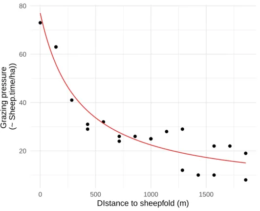
Characterizing the grazing gradient

266

In La Crau, the local grazing pressure (the number of sheep*time unit.ha-1) is known to decrease with 267

the distance to the sheepfold, but this relationship has not been explicitly measured for most sites. 268

Previous studies (Dureau 1998; Supplementary Information 2) suggest that it decreases as the inverse 269

of distance then reaches a minimum, i.e. that grazing pressure 𝐺 can be described by the following 270 function: 271 𝐺(𝑥) = 𝐺_𝑖𝑛𝑓+𝐺0−𝐺𝑖𝑛𝑓 1+𝜏𝑥 = 𝜏𝐺0+𝑥𝐺𝑖𝑛𝑓 𝜏+𝑥 (equation 1) 272

where 𝑥 is the distance to the sheepfold, 𝐺𝑖𝑛𝑓 is the grazing pressure far from the sheepfold, 𝐺0is the

273

grazing pressure at the sheepfold, and 𝜏 characterizes the spatial extent of the gradient. 274

275

Soil characteristics are expected to follow closely the grazing pressure. This is particularly true for soil 276

nutrients that are spatially redistributed as grazers feed in a given area and defecate in another 277

(Steinauer and Collins 1995, Selbie et al. 2015). In our area, we thus expected the variations in the 278

amount of nutrients in the soil to closely match those in grazing pressure. We therefore carried out 279

sampling to measure soil properties as a function of the distance to the sheepfold. We sampled soil 280

wherever a pair of transects was carried out, and complemented these samples with additional ones 281

where the grazing gradient was very extended (see Supplementary Information 1). Soil was sampled by 282

mixing subsamples of the upper first five centimeters (after scraping sheep dung) from a circular area 283

of radius 4 m. Soil sampling took place in October 2017, when sheep flocks were absent. 284

285

We used the total Nitrogen content (𝑁_𝑡𝑜𝑡) in the soil (as measured by the Kjeldahl method; Bremner 286

1960) to characterize the grazing pressure at a given distance from the sheepfold. We assumed that the 287

total 𝑁 measured from soil samples was linearly-related to the (unmeasured) grazing pressure, i.e. that 288

𝑁_𝑡𝑜𝑡 = 𝑎𝐺(𝑥) + 𝑏 (with 𝑎 and 𝑏 being the slope and the intercept, respectively). Based on equation 1, 289

this yields the expected relationship between distance 𝑥 and nitrogen content 𝑁_𝑡𝑜𝑡, which we fitted to 290

the empirical data: 291

𝑁_𝑡𝑜𝑡(𝑥) =𝜏𝑁𝑡𝑜𝑡,0+𝑥𝑁𝑡𝑜𝑡,𝑖𝑛𝑓

𝜏+𝑥 (equation 2)

292

Because we had a reduced number of samples per site (2 to 4) and standard non-linear regression was 293

prone to overfitting, we carried out the regression using a Bayesian setting and weakly conservative 294

priors. We used the site as a random effect on the estimates of 𝜏, 𝑁𝑡𝑜𝑡,0 and 𝑁𝑡𝑜𝑡,𝑖𝑛𝑓 along with a

295

Gaussian residual error (see Supplementary Information 2 for details on parameter estimation). 296

We checked that the estimated values for 𝑁_{𝑡𝑜𝑡,0} and 𝑁_{𝑡𝑜𝑡,𝑖𝑛𝑓} were consistent with previous reported 297

values for the area (Römermann et al. 2005), and then used the estimated 𝑁𝑡𝑜𝑡in the soil at the given

298

distance to the sheepfold as a proxy for grazing pressure. 299

300

Effect of grazing pressure on associations

301 302

We characterized the effect of grazing on species associations by investigating the trends of 303

community-level metrics along the gradient of grazing pressure (as measured by 𝑁_𝑡𝑜𝑡). To test whether 304

the trends were linear or unimodal (hump-shaped), we fitted both a straight-slope and a second-order 305

polynomial model, with the focal metric as response (e.g. 𝑅_𝑆𝐸𝑆), the estimated 𝑁_𝑡𝑜𝑡as predictor and the 306

site as a random effect on the trend coefficients. We carried out this regression using a Bayesian setting 307

with uninformative priors, and retained the model that had the lowest error when carrying leave-one-308

out (loo) cross-validation, following recommendations from Vehtari et al. (2017). We used normal 309

priors with mean zero and standard deviation 50 for regression coefficients, and an exponential prior 310

with rate 0.1 for the residual error parameter. 311

312

All analyses were carried out in R v4.0.2 (R Core Team 2020), with regressions carried out using the 313

package loo v2.3.1 (Vehtari et al. 2017) and brms v2.14.0 (Bürkner 2017). Data and code used for the 314

analyses are available at https://datadryad.org/stash/dataset/doi:10.5061/dryad.ns1rn8prd [private 315

during peer-review]. Trait data to compute the percentage of ruderal species was obtained from the

316

TRY database (Kühn et al. 2004, Kattge et al. 2020). 317

Results

319

We found that the grazing gradient around sheepfolds had a strong effect on soil conditions, as total 320

nitrogen of the soil was doubled (model estimation of 1.35 ± 0.36 g.kg-1 far from sheepfolds vs. 321

2.85 ± 0.27 g.kg-1 _{at the entrance; Figure 3a). Such values are consistent with what has been previously}

322

reported in the study area (Römermann et al. 2005, Saatkamp et al. 2020). The effects of grazing on 323

soil surface conditions were evidenced by the increase in bare ground from 20 ± 7 % to 42 ± 14 % 324

(Figure 3b) and dung cover from 9 ± 5 % to 92 ± 12 % (Figure 3c). Grazing favored higher covers of 325

ruderal species (17 ± 8 % to 63 ± 5 %, Figure 3d) and reduced species richness (49 ± 6 species far, vs 326

10 ± 1 close to sheepfolds; Figure 3e). 327

328

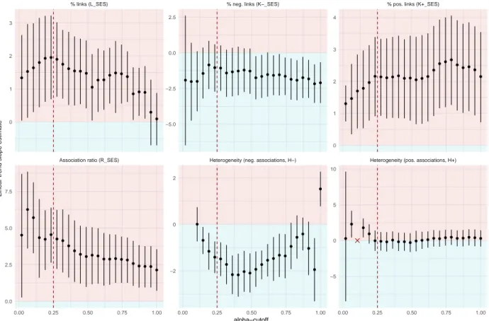
Regarding plant association metrics, model selection favored linear relationships (straight lines) for all 329

relationships between association-based community-level metrics and grazing pressure (Figure 4,5). In 330

particular, we found no support for unimodal variations of the number of positive associations 𝐾_𝑆𝐸𝑆+ 331

along the gradient (Figure 4c). 332

333

Grazing was found to increase the number of links in plant communities (LSES, Figure 4a), as positive

334

associations decayed quicker than negative associations with grazing (Figure 4b, 4c). Overall, there 335

was an excess of negative associations compared to positive associations (𝐾_𝑆𝐸𝑆− _{was always above zero}

336

and 𝐾_𝑆𝐸𝑆+ _{almost always below zero; Figure 4b, 4c). Both negative and positive associations were found}

337

to approach the null expectation (i.e. a value of 𝐾_𝑆𝐸𝑆− _{and 𝐾}

𝑆𝐸𝑆+ close to zero) as sheep pressure

338

increased (Figure 4b, 4c). Consistent with these patterns, the association ratio 𝑅𝑆𝐸𝑆 was always

339

negative regardless of the grazing level, and close to the null expectation where grazing was the highest 340

(Figure 4d). This suggests that these communities were strongly structured by spatial associations at 341

low grazing pressure, but became increasingly close to the null expectation with increased grazing. 342

343

The heterogeneity in negative associations 𝐻_𝑆𝐸𝑆− _{decreased with grazing pressure (Figure 5a). In other}

344

words, plant species of a given community had similar numbers of negative associations with each 345

other under high grazing conditions and more variable ones under low grazing. We found no equivalent 346

effect of grazing on the heterogeneity of positive associations 𝐻_𝑆𝐸𝑆+ _{(Figure 5b).}

347 348

All the above trends were robust to the choice of 𝛼 (Supplementary Information 3). 349

350 351 352

Discussion

353

Using continuous transects documenting the spatial associations of plant individuals in a Mediterranean 354

dry grassland, we found non-random trends in spatial associations along the grazing intensity gradient. 355

Negative associations were found to dominate over positive ones under low grazing, with a highly-356

variable number of negative association per species. Grazing was found to reduce all these 357

characteristics to their null expectations, overall making the communities less structured by 358

interspecific associations at high grazing levels. 359

360

Association trends

361

Changes in association trends

362

We found that negative associations dominated where grazing pressure was lower (H1), which is 363

consistent with interference driving the assembly of communities (Graff et al. 2007). As grazing 364

pressure increases, it appears that this imprint of interference on spatial patterns vanishes. This is 365

consistent with the known effects of grazing in grasslands: as biomass is removed from dominant 366

species, ground-level light increases and thus spatial exclusion by taller competitors is reduced (Borer 367

et al. 2014, Odriozola et al. 2017). However, such decrease in negative interactions is usually 368

associated with an increase in species richness that we did not observe here (Figure 3e). This suggests 369

that the trends observed here reflect more than a sole reduction in interference. Given the very high 370

disturbance levels around sheepfolds (more than 1000 sheep being present daily close to sheepfolds), 371

another factor altering spatial patterns is the direct reduction in covers due to the sheep presence (Adler 372

et al. 2001, Graff and Aguiar 2011). Disturbance may be too high to allow plants to grow enough 373

during the grazing season to preempt space and produce significant spatial patterns (Alados et al. 374

2004). Disentangling this direct effect of disturbance on spatial associations from that of the processes 375

occurring within the plant community would require additional independent evidence, and constitutes a 376

limit of relying only on association networks. 377

378

Positive associations exhibited no unimodal trend along the grazing gradient (H2). Instead, we found 379

that they declined linearly with increasing grazing. This contrasts with previous work reporting 380

unimodal trends along grazing gradients both experimentally (Smit et al. 2009) and using association 381

(Saiz and Alados 2012, Le Bagousse-Pinguet et al. 2012). A possible explanation for this pattern is that 382

our study was carried out in areas where the grazing pressure is always relatively high compared to 383

other work using association networks. Stocking rates in La Crau often reach above 1 ind.ha-1 (Buisson 384

et al. 2015), well above the maximum rate of 0.64 ind.ha-1 reported by Saiz et al. (2012). It is thus 385

likely that we could only document the reduction in the importance of interactions under high 386

disturbance, as suggested by Graff et al. (2013). Moreover, positive associations were found to be less 387

frequent than expected by chance at all grazing levels, suggesting that facilitation is rare in our system. 388

This general absence of facilitation, despite some existing experimental evidence (Buisson et al. 2015), 389

could emerge from the particular morphology of the plants in the study area. The study area lacks tall 390

woody shrubs which are a major source of positive associations, as they often act as nurse species 391

under which herbaceous plants grow in dry areas (Saiz and Alados 2012). Compared to the study of 392

Saiz and Alados (2012), at our sites, plants are more functionally similar (forbs and grasses of similar 393

heights), which limits the possibility of plants to aggregate in space by growing on top of, or below, 394

each other, and thus the proportion of positive associations. This could explain in particular why the 395

species Brachypodium retusum, which exhibits mostly negative associations in our work, was found to 396

engage mostly in positive ones in Saiz and Alados (2012). By reducing the necessary complementarity 397

in height and morphology of the plants for spatial aggregation, i.e. increasing functional similarity, 398

grazing could reduce the prevalence of positive associations in our study area. 399

400

Heterogeneity in associations

While plant ecology has mostly focused on describing the relative importance of different types of 402

interactions (e.g. the relative importance of facilitation vs. interference; Callaway et al. 2002, Michalet 403

et al. 2006, Soliveres et al. 2015), it has seldom focused on the structural aspects of plant-plant 404

interaction networks. For example, facilitation in abiotically-stressed environments can be asymmetric, 405

with key nurse plants facilitating many others, or more symmetric, where plants with similar lifeforms 406

buffer each other against harsh conditions (Lin et al. 2012). In our study, such asymmetry was found in 407

negative associations. We found that they were more heterogeneous when grazing was low. This 408

suggests that under low grazing conditions, inter-specific interference is asymmetric, with few species 409

establishing a high number of negative links, and does not arise from all plants being equally more 410

competitive. This maps well onto limiting-similarity acting where competition for resources dominates 411

(Chesson 2000), which favors functional divergence in traits (Valiente-Banuet and Verdú 2008) and 412

plant strategies. Some plants may engage in “Competitive confrontation” (sensu Novoplansky 2009) by 413

maximizing interference with their neighbors, while other may display “Competitive avoidance” or 414

tolerance and avoid such behavior (Gruntman et al. 2017). This diversity in plant strategies may be a 415

factor explaining the heterogeneity in negative links. As grazing increases, communities converge 416

towards grazing-tolerant strategies (Carmona et al. 2012 and Figure 3d), resulting in the observed 417

reduction of network heterogeneity. Such hypotheses could be tested with theoretical models exploring 418

the link between plant traits and strategies, and the structure of interaction networks in plant 419

communities. More generally, this line of thought could also be extended to other network properties 420

such as modularity, nestedness (Verdú and Valiente-Banuet 2008) or structural balance (Saiz et al. 421

2017). Research on food webs has produced several of such theoretical models of network assembly 422

from species traits (e.g. Williams and Martinez 2000): equivalent work for plant association networks 423

is still burgeoning (Lin et al. 2012). 424

Moving forward with associations

426

Using associations as proxies to estimate plant-plant interactions seems to have been deemed a 427

reasonable solution for plants in arid drylands, as evidenced by the breadth of papers relying on this 428

method (e.g. Verdú and Valiente‐Banuet 2008, Saiz and Alados 2012, Delalandre and Montesinos-429

Navarro 2018). This may be motivated by the fact that facilitation (e.g. between nurse plants and their 430

protected species, a type of interaction which is particularly frequent in arid ecosystems) has been 431

shown to be well-captured by association patterns (Freilich et al. 2018). However, our work suggests 432

that plant-plant associations provide valuable information in other ecosystems as well. Strengthening 433

this approach further would require additional evidence to assess whether interactions in a community 434

effectively give rise to the expected association patterns. Such piece of evidence could come from 435

independent trait data (Soliveres et al. 2014). For example, increased functional similarity between two 436

plants could be associated with a higher likelihood of observing a negative association between them 437

(Conti et al. 2017). Another avenue to put the association approach to the test would be to rely on 438

experimental approaches directly measuring interaction strengths (Choler et al. 2001). Given the 439

ballooning number of studies based on plant associations (Losapio et al. 2019), it becomes more and 440

more timely to test such assumptions. 441

442

Another hurdle lying ahead of association-based work is methodological in nature. Much work outside 443

of plant ecology shows that many factors can bias the interaction strengths estimated from spatial 444

associations, such as the scale of sampling (Araújo and Rozenfeld 2014, McNickle et al. 2018, 445

Delalandre and Montesinos-Navarro 2018), the species’ habitat preferences (Morueta-Holme et al. 446

2016) or the method used for inference (Barner et al. 2018). Working at the local scale, where the 447

imprint of ecological interactions is generally thought to be stronger, and with sessile species may 448

alleviate some of those shortcomings, but probably not all of them. For example, shared residual 449

differences in micro-habitat may drive some of the associations between species. Here, our sampling 450

avoided any apparent fine-scale variations in soil characteristics, but residual bias may still be present. 451

For example, in our transects, the presence of pebbles (typical size of 5-20 cm) may make plant 452

individuals only grow in those remaining areas where pebbles are not present. This can produce 453

artefactual positive associations that are not due to any biotic interaction, as plant will cluster in the 454

remaining areas with free bare ground. In our case, this effect is unlikely to affect the trends given the 455

large predominance of negative associations, but it highlights the limits to the precision of association-456

based approaches. 457

458

Relying on spatial patterns to make general statements about interactions in plant communities will 459

also require a standardization of methods. One acute point worth highlighting when considering trends 460

in association networks along gradients is controlling for changes in species abundances (Pellissier et 461

al. 2018). If networks are being compared without correction, the trends may not reflect changes in 462

species’ behaviors but rather changes in cover. For example, rare species cannot produce negative 463

associations, because even though they may strongly exclude other species in space, their total cover is 464

not sufficient to produce significant spatial segregation (Supplementary Information 4). Reporting 465

ecologically-meaningful variations in community-level metrics (e.g. the total number of negative links, 466

𝐾−_{) must be done with indices that control for species covers (e.g. 𝐾}

𝑆𝐸𝑆− ). Misinterpreting this property

467

of associations can lead and has led to spurious interpretation of patterns (e.g. Calatayud et al. 2020). 468

469

To adequately anticipate how ecological communities will respond to global changes, it is necessary to 470

better map empirical interaction networks. This may not always be possible, as pairwise experiments 471

may be prohibitively expensive, or previous knowledge may be missing for the ecosystem of interest 472

(e.g. Kéfi et al. 2015). Association-based approaches provide an alternative yet objective basis to map 473

interactions in situ, preserving the environmental setting in which they occur, and for systems where 474

previous knowledge is scarce. They could thus greatly complement traditional approaches, but come 475

with their own sets of methodological challenges. Obtaining detailed and accurate empirical interaction 476

networks will thus require leveraging the complementarity of both experimental and observational 477 approaches. 478 479

References

Adler, P. et al. 2001. The effect of grazing on the spatial heterogeneity of vegetation. - Oecologia 128: 481

465–479. 482

Alados, C. L. et al. 2004. Change in plant spatial patterns and diversity along the successional gradient 483

of Mediterranean grazing ecosystems. - Ecol. Model. 180: 523–535. 484

Araújo, M. B. and Rozenfeld, A. 2014. The geographic scaling of biotic interactions. - Ecography 37: 485

406–415. 486

Badan, O. et al. 1995. Les bergeries romaines de la Crau d’Arles. Les origines de la transhumance en 487

Provence. - Gallia 52: 263–310. 488

Baraza, E. et al. 2006. Conditional outcomes in plant–herbivore interactions: neighbours matter. - 489

Oikos 113: 148–156. 490

Barner, A. K. et al. 2018. Fundamental contradictions among observational and experimental estimates 491

of non-trophic species interactions. - Ecology 99: 557–566. 492

Blanchet, F. G. et al. 2020. Co‐occurrence is not evidence of ecological interactions. - Ecol. Lett. 23: 493

1050–1063. 494

Borer, E. T. et al. 2014. Herbivores and nutrients control grassland plant diversity via light limitation. - 495

Nature 508: 517–520. 496

Bremner, J. M. 1960. Determination of nitrogen in soil by the Kjeldahl method. - J. Agric. Sci. 55: 11– 497

33. 498

Buisson, E. and Dutoit, T. 2006. Creation of the natural reserve of La Crau: Implications for the 499

creation and management of protected areas. - J. Environ. Manage. 80: 318–326. 500

Buisson, E. et al. 2015. Limiting processes for perennial plant reintroduction to restore dry grasslands: 501

Perennial plant reintroduction in dry grasslands. - Restor. Ecol. 23: 947–954. 502

Bürkner, P.-C. 2017. brms: An R package for Bayesian multilevel models using Stan. - J. Stat. Softw. 503

80: 1–28. 504

Calatayud, J. et al. 2020. Positive associations among rare species and their persistence in ecological 505

assemblages. - Nat. Ecol. Evol. 4: 40–45. 506

Callaway, R. M. 2007. Positive interactions and interdependence in plant communities. - Springer. 507

Callaway, R. M. et al. 2002. Positive interactions among alpine plants increase with stress. - Nature 508

417: 844–848. 509

Carmona, C. P. et al. 2012. Taxonomical and functional diversity turnover in Mediterranean 510

grasslands: interactions between grazing, habitat type and rainfall. - J. Appl. Ecol. 49: 1084– 511

1093. 512

Chesson, P. 2000. Mechanisms of maintenance of species diversity. - Annu. Rev. Ecol. Syst. 31: 343– 513

366. 514

Choler, P. et al. 2001. Facilitation and competition on gradients in alpine plant communities. - Ecology 515

82: 3295–3308. 516

Conti, L. et al. 2017. Environmental gradients and micro-heterogeneity shape fine-scale plant 517

community assembly on coastal dunes. - J. Veg. Sci. 28: 762–773. 518

D’Amen, M. et al. 2018. Disentangling biotic interactions, environmental filters, and dispersal 519

limitation as drivers of species co-occurrence. - Ecography 41: 1233–1244. 520

Delalandre, L. and Montesinos-Navarro, A. 2018. Can co-occurrence networks predict plant-plant 521

interactions in a semi-arid gypsum community? - Perspect. Plant Ecol. Evol. Syst. 31: 36–43. 522

Devaux, J. et al. 1983. Notice de la carte phyto-écologique de la Crau (Bouches du Rhône). - Biol. 523

Écologie Méditerranéenne 10: 5–54. 524

Díaz, S. et al. 2007. Plant trait responses to grazing: a global synthesis. - Glob. Change Biol. 13: 313– 525

341. 526

Díaz-Sierra, R. et al. 2017. A new family of standardized and symmetric indices for measuring the 527

intensity and importance of plant neighbour effects. - Methods Ecol. Evol. 8: 580–591. 528

Dureau, R. 1998. Conduite pastorale et répartition de l’avifaune nicheuse des coussouls. Patrimoine 529

naturel et pratiques pastorales en Crau - Rapport du programme LIFE ACE Crau.: 90–97. 530

Engel, E. C. and Weltzin, J. F. 2008. Can community composition be predicted from pairwise species 531

interactions? - Plant Ecol. 195: 77–85. 532

Estrada, E. 2010. Quantifying network heterogeneity. - Phys. Rev. E 82: 066102. 533

Freilich, M. A. et al. 2018. Species co-occurrence networks: Can they reveal trophic and non-trophic 534

interactions in ecological communities? - Ecology 99: 690–699. 535

Graff, P. and Aguiar, M. R. 2011. Testing the role of biotic stress in the stress gradient hypothesis. 536

Processes and patterns in arid rangelands. - Oikos 120: 1023–1030. 537

Graff, P. et al. 2007. Shifts in positive and negative plant interactions along a grazing intensity 538

gradient. - Ecology 88: 188–199. 539

Graff, P. et al. 2013. Changes in sex ratios of a dioecious grass with grazing intensity: the interplay 540

between gender traits, neighbour interactions and spatial patterns. - J. Ecol. 101: 1146–1157. 541

Grime, J. P. 1977. Evidence for the existence of three primary strategies in plants and its relevance to 542

ecological and evolutionary theory. - Am. Nat. 111: 1169–1194. 543

Gruntman, M. et al. 2017. Decision-making in plants under competition. - Nat. Commun. 8: 2235. 544

Guimarães, P. R. 2020. The Structure of Ecological Networks Across Levels of Organization. - Annu. 545

Rev. Ecol. Evol. Syst. 51: annurev-ecolsys-012220-120819. 546

Holthuijzen, M. F. and Veblen, K. E. 2016. Grazing effects on precipitation-driven associations 547

between sagebrush and perennial grasses. - West. North Am. Nat. 76: 313–325. 548

Kattge, J. et al. 2020. TRY plant trait database – enhanced coverage and open access. - Glob. Change 549

Biol. 26: 119–188. 550

Kéfi, S. et al. 2007. Spatial vegetation patterns and imminent desertification in Mediterranean arid 551

ecosystems. - Nature 449: 213–217. 552

Kéfi, S. et al. 2015. Network structure beyond food webs: mapping non-trophic and trophic interactions 553

on Chilean rocky shores. - Ecology 96: 291–303. 554

Kühn, I. et al. 2004. BiolFlor - a new plant-trait database as a tool for plant invasion ecology: BiolFlor 555

- a plant-trait database. - Divers. Distrib. 10: 363–365. 556

Le Bagousse-Pinguet, Y. et al. 2012. Release from competition and protection determine the outcome 557

of plant interactions along a grazing gradient. - Oikos 121: 95–101. 558

Levine, J. M. et al. 2017. Beyond pairwise mechanisms of species coexistence in complex 559

communities. - Nature 546: 56–64. 560

Lin, Y. et al. 2012. Differences between symmetric and asymmetric facilitation matter: exploring the 561

interplay between modes of positive and negative plant interactions. - J. Ecol. 100: 1482–1491. 562

Losapio, G. et al. 2019. Perspectives for ecological networks in plant ecology. - Plant Ecol. Divers.: 1– 563

17. 564

Maestre, F. T. et al. 2009. Refining the stress-gradient hypothesis for competition and facilitation in 565

plant communities. - J. Ecol. 97: 199–205. 566

McNickle, G. G. et al. 2018. Checkerboard score-area relationships reveal spatial scales of plant 567

community structure. - Oikos 127: 415–426. 568

Michalet, R. et al. 2006. Do biotic interactions shape both sides of the humped-back model of species 569

richness in plant communities? - Ecol. Lett. 9: 767–773. 570

Molinier, R. and Tallon, G. 1950. La végétation de la Crau. - Rev. Générale Bot.: 525–540. 571

Morueta-Holme, N. et al. 2016. A network approach for inferring species associations from co-572

occurrence data. - Ecography 39: 1139–1150. 573

Novoplansky, A. 2009. Picking battles wisely: plant behaviour under competition. - Plant Cell Environ. 574

32: 726–741. 575

Odriozola, I. et al. 2017. Grazing exclusion unleashes competitive plant responses in Iberian Atlantic 576

mountain grasslands. - Appl. Veg. Sci. 20: 50–61. 577

Pellissier, L. et al. 2018. Comparing species interaction networks along environmental gradients: 578

Networks along environmental gradients. - Biol. Rev. 93: 785–800. 579

R Core Team 2020. R: A Language and Environment for Statistical Computing. - R Foundation for 580

Statistical Computing. 581

Rajala, T. et al. 2019. When do we have the power to detect biological interactions in spatial point 582

patterns? - J. Ecol. 107: 711–721. 583

Römermann, C. et al. 2005. Influence of former cultivation on the unique Mediterranean steppe of 584

France and consequences for conservation management. - Biol. Conserv. 121: 21–33. 585

Saatkamp, A. et al. 2020. Romans Shape Today’s Vegetation and Soils: Two Millennia of Land-Use 586

Legacy Dynamics in Mediterranean Grasslands. - Ecosystems in press. 587

Saiz, H. and Alados, C. L. 2011. Structure and spatial self-organization of semi-arid communities 588

through plant–plant co-occurrence networks. - Ecol. Complex. 8: 184–191. 589

Saiz, H. and Alados, C. L. 2012. Changes in semi-arid plant species associations along a livestock 590

grazing gradient. - PloS One 7: e40551. 591

Saiz, H. et al. 2017. Evidence of structural balance in spatial ecological networks. - Ecography 40: 592

733–741. 593

Saiz, H. et al. 2018. The structure of plant spatial association networks is linked to plant diversity in 594

global drylands. - J. Ecol. 106: 1443–1453. 595

Sanderson, J. G. and Pimm, S. L. 2015. Patterns in nature: the analysis of species co-occurrences. - The 596

University of Chicago Press. 597

Selbie, D. R. et al. 2015. The Challenge of the Urine Patch for Managing Nitrogen in Grazed Pasture 598

Systems. - In: Advances in Agronomy. Elsevier, pp. 229–292. 599

Smit, C. et al. 2009. Inclusion of biotic stress (consumer pressure) alters predictions from the stress 600

gradient hypothesis. - J. Ecol. 97: 1215–1219. 601

Soliveres, S. and Maestre, F. T. 2014. Plant–plant interactions, environmental gradients and plant 602

diversity: A global synthesis of community-level studies. - Perspect. Plant Ecol. Evol. Syst. 16: 603

154–163. 604

Soliveres, S. et al. 2014. Functional traits determine plant co-occurrence more than environment or 605

evolutionary relatedness in global drylands. - Perspect. Plant Ecol. Evol. Syst. 16: 164–173. 606

Soliveres, S. et al. 2015. Moving forward on facilitation research: response to changing environments 607

and effects on the diversity, functioning and evolution of plant communities: Facilitation, 608

community dynamics and functioning. - Biol. Rev. 90: 297–313. 609

Steinauer, E. M. and Collins, S. L. 1995. Effects of Urine Deposition on Small-Scale Patch Structure in 610

Prairie Vegetation. - Ecology 76: 1195–1205. 611

Thebault, E. and Fontaine, C. 2010. Stability of Ecological Communities and the Architecture of 612

Mutualistic and Trophic Networks. - Science 329: 853–856. 613

Tielbörger, K. and Kadmon, R. 2000. Temporal environmental variation tips the balance between 614

facilitation and interference in desert plants. - Ecology 81: 1544–1553. 615

Tilman, D. 1982. Resource competition and community structure. - Princeton university press. 616

Tylianakis, J. M. and Morris, R. J. 2017. Ecological networks across environmental gradients. - Annu. 617

Rev. Ecol. Evol. Syst. 48: 25–48. 618

Valiente-Banuet, A. and Verdú, M. 2008. Temporal shifts from facilitation to competition occur 619

between closely related taxa. - J. Ecol. 96: 489–494. 620

Vehtari, A. et al. 2017. Practical Bayesian model evaluation using leave-one-out cross-validation and 621

WAIC. - Stat. Comput. 27: 1413–1432. 622

Verdú, M. and Valiente‐Banuet, A. 2008. The Nested Assembly of Plant Facilitation Networks 623

Prevents Species Extinctions. - Am. Nat. 172: 751–760. 624

Vries, D. M. 1954. Constellation of frequent herbage plants, based on their correlation in occurrence: 625

with 1 table and 2 figures. - Vegetatio 5–6: 105–111. 626

Williams, R. J. and Martinez, N. D. 2000. Simple rules yield complex food webs. - Nature 404: 180– 627

183. 628

Wootton, J. T. 1994. The nature and consequences of indirect effects in ecological communities. - 629

Annu. Rev. Ecol. Syst. 25: 443–466. 630

Figures

632 633

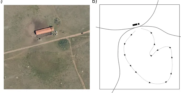
634

Figure 1. General variation of vegetation around a sheepfold and procedure used to calculate 635

community-level network properties. Vegetation can be divided into different “belts” (a1), whose 636

spatial extents depend on the grazing pressure (a2) and which are most extended towards the south-east 637

because of the sheepfold buffering the herds against dominant winds (a1). We carried out two transects 638

per vegetation type (i.e. per belt) in the south-east direction, leading to one observed association 639

network and 999 ‘null’ networks per pair of transect (b1). Both observed and null networks were 640

summarized into summary metrics, for example 𝑅, the relative frequency of positive to negative 641

associations (b2). The deviation of the observed summary metric from the null expectation was then 642

computed using standardized effect size, yielding cover-corrected community-level metrics such as 643

𝑅𝑆𝐸𝑆 (b3).

644 645

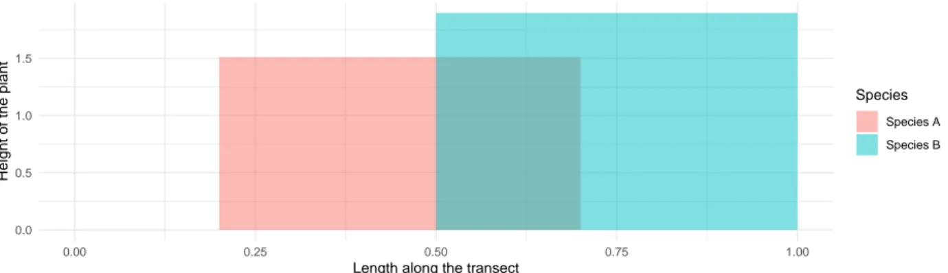
Figure 2. Design of the transect surveys. Panel (a) represents a top-down view of plant individuals 647

spread along a line transect (black line). We recorded all intersections of the line with plant parts, along 648

with a class of height (b). The total overlap between species was then computed along the transect. For 649

example, here 𝑂₁₂, the total overlap between species 1 and 2 is given by 𝑂₁₂ = 𝑙₁+ 𝑙₂. We used pairs 650

of transects in the field but in this figure, only one transect is represented for simplicity. 651

Figure 3. Variations in soil nitrogen, bare ground, dung cover, percentage of ruderal species, species 653

richness as a function of distance to the sheepfold. The shape of the points and the separate trend lines 654

indicate the different sites. Red trend lines are fits of a saturating function (the relationship described in 655

equation 2), with different link functions depending on the nature of the response variable 656

(proportional, continuous or discrete). The percentage of ruderal species is the proportion of the total 657

plant cover made up of ruderal species sensu Grime’s CSR classification (Grime 1977). 658

Figure 4. Total fraction of links (𝐿_𝑆𝐸𝑆), fraction of negative (𝐾_𝑆𝐸𝑆− _{), positive links (𝐾}

𝑆𝐸𝑆+ ) and association

661

ratio (𝑅_𝑆𝐸𝑆) as a function of grazing pressure. Trend lines indicate linear regressions along the grazing 662

gradient, as measured through total Nitrogen, with dashed lines representing the 95% credible interval 663

on the predicted mean. Red and blue backgrounds highlight the areas corresponding to positive and 664

negative values, respectively. Point shapes indicate different sites. 665

666

667

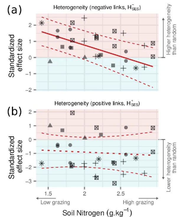
Figure 5. Trends of the heterogeneity of negative (𝐻_𝑆𝐸𝑆− _{, a) and positive (𝐻}

𝑆𝐸𝑆+ , b) links. Red and blue

backgrounds highlight the areas corresponding to positive and negative values, respectively. Trend 669

lines indicate linear regressions along the grazing gradient, as measured through total Nitrogen, with 670

dashed lines representing the 95% credible interval on the predicted mean. The posterior distribution 671

for the 𝐻_𝑆𝐸𝑆+ _{slope included zero between its 2.5% and 97.5% quantiles, suggesting no effect of grazing,}

672

so the trend is represented with a dotted line. 673