HAL Id: insu-02275907
https://hal-insu.archives-ouvertes.fr/insu-02275907
Submitted on 19 Sep 2019
HAL is a multi-disciplinary open access
archive for the deposit and dissemination of
sci-entific research documents, whether they are
pub-lished or not. The documents may come from
teaching and research institutions in France or
L’archive ouverte pluridisciplinaire HAL, est
destinée au dépôt et à la diffusion de documents
scientifiques de niveau recherche, publiés ou non,
émanant des établissements d’enseignement et de
recherche français ou étrangers, des laboratoires
muon detector
M. Tramontini, Marina Rosas-carbajal, C. Nussbaum, Dominique Gibert,
Jacques Marteau
To cite this version:
M. Tramontini, Marina Rosas-carbajal, C. Nussbaum, Dominique Gibert, Jacques Marteau.
Middle-atmosphere dynamics observed with a portable muon detector. Earth and Space Science, American
Geophysical Union/Wiley, 2019, 6 (10), pp.1865-1876. �10.1029/2019EA000655�. �insu-02275907�
Middle-atmosphere dynamics observed with a portable
1
muon detector
2
M. Tramontini1,2, M. Rosas-Carbajal3, C. Nussbaum4, D. Gibert5, J.
3
Marteau1
4
1Institut de Physique Nucl´eaire de Lyon, UMR 5822, CNRS-IN2P3, Universit´e de Lyon, Universit´e
5
Claude Bernard Lyon 1, France
6
2CONICET - Facultad de Ciencias Astron´omicas y Geof´ısicas, Universidad Nacional de La Plata,
7
Argentina
8
3Universit´e de Paris, Institut de Physique du Globe de Paris, CNRS, UMR 7154, F-75238 Paris, France
9
4Swiss Geological Survey at swisstopo, Seftigenstrasse 264, CH-3084 Wabern, Switzerland
10
5Univ. Rennes, CNRS, G´eosciences Rennes, UMR 6118, F-35000, Rennes, France
11
Key Points: 12
• We report muon rate variations associated to temperature changes in the middle 13
atmosphere observed with a portable muon detector 14
• The effect is significant both for seasonal and short-term temperature variations, 15
even under low-opacity conditions at mid-latitudes 16
• We highlight potential applications on atmosphere dynamics and the need to ac-17
count for these phenomena in geophysical applications 18
Corresponding author: Marina Rosas-Carbajal, [email protected]
This article has been accepted for publication and undergone full peer review but has not been
through the copyediting, typesetting, pagination and proofreading process which may lead to
differences between this version and the Version of Record. Please cite this article as doi:
Abstract 19
In the past years, large particle-physics experiments have shown that muon rate variations 20
detected in underground laboratories are sensitive to regional, middle-atmosphere temper-21
ature variations. Potential applications include tracking short-term atmosphere dynamics, 22
such as Sudden Stratospheric Warmings. We report here that such sensitivity is not only 23
limited to large surface detectors under high-opacity conditions. We use a portable muon 24
detector conceived for muon tomography for geophysical applications and we study muon 25
rate variations observed over one year of measurements at the Mont Terri Underground Rock 26
Laboratory, Switzerland (opacity of ∼ 700 meter water equivalent). We observe a direct cor-27
relation between middle-atmosphere seasonal temperature variations and muon rate. Muon 28
rate variations are also sensitive to the abnormal atmosphere heating in January-February 29
2017, associated to a Sudden Stratospheric Warming. Estimates of the effective temperature 30
coefficient for our particular case agree with theoretical models and with those calculated 31
from large neutrino experiments under comparable conditions. Thus, portable muon de-32
tectors may be useful to 1) study seasonal and short-term middle atmosphere dynamics, 33
especially in locations where data is lacking such as mid-latitudes; and 2) improve the cali-34
bration of the effective temperature coefficient for different opacity conditions. Furthermore, 35
we highlight the importance of assessing the impact of temperature on muon rate variations 36
when considering geophysical applications. Depending on latitude and opacity conditions, 37
this effect may be large enough to hide subsurface density variations due to changes in 38
groundwater content, and should therefore be removed from the time-series. 39
1 Introduction
40First observed in 1952 using radiosonde measurements (Scherhag, 1952), Sudden Strato-41
spheric Warmings (SSWs) are extreme wintertime circulation anomalies that produce a 42
rapid rise in temperature in the mid to upper polar stratosphere (30-50 km). SSW ef-43
fects on middle-atmosphere dynamics have lifetimes of approximately 80 days (Limpasuvan, 44
Thompson, & Hartmann, 2004). They are the clearest and strongest manifestation of dy-45
namic coupling throughout the whole atmosphere-ocean system (Goncharenko, Chau, Liu, 46
& Coster, 2010; Liu & Roble, 2002; O’Callaghan, Joshi, Stevens, & Mitchell, 2014). Follow-47
ing a major SSW, the high altitude winds reverse to flow westward instead of their usual 48
eastward direction. This reversal often results in dramatic surface temperature reductions 49
in mid-latitudes, particularly in Europe, which suggests the possibility of monitoring the 50
stratosphere for predicting extreme tropospheric weather (Thompson, Baldwin, & Wallace, 51
2002). The frequency of SSWs may increase due to global warming (Kang & Tziperman, 52
2017; Schimanke, Spangehl, Huebener, & Cubasch, 2013). While many studies have focused 53
on the characterization of SSWs through observation and modeling dynamics at high lat-54
itude regions, observation studies at mid-latitudes are rare and could be crucial to better 55
understand the phenomena (Sox, Wickwar, Fish, & Herron, 2016; Yuan et al., 2012). 56
Cosmic muons represent the largest proportion of charged particles reaching the surface 57
of the Earth, yielding a flux of ∼ 70 m−2s−1sr−1 for particles above 1 GeV (Tanabashi et 58
al., 2018). They are a product of the primary cosmic rays interaction with the atmosphere, 59
which produces short-lived mesons, in particular, charged pions and kaons. These particles 60
decay into muons that easily penetrate the atmosphere and may reach the surface of the 61
Earth. The flux of muons decreases as muons travel through an increasing amount of matter. 62
Thus, only the most energetic muons can reach underground detectors (Gaisser, Engel, & 63
Resconi, 2016). The muon production process requires that the parent mesons did not 64
undergo destructive interactions with the propagating medium before they decay (Grashorn 65
et al., 2010). Thus, changes in the atmospheric properties, in particular in its density, may 66
have large impacts on the muon flux measured at ground level, either by affecting the parent 67
mesons survival probabilities before decay or by affecting the rate of absorption of the muons 68
themselves along their path down from their production level. 69
An increase in the atmospheric temperature lowers the atmospheric density. Temper-70
ature changes in the atmosphere may therefore affect the production of muons (Gaisser et 71
al., 2016). The decrease in atmospheric density increases the mean free path of the mesons 72
and therefore their decay probability, thus increasing the muon flux. The effect is more 73
important for high-energy muons, which result from high-energy mesons with larger lifetime 74
due to time dilation and therefore with longer paths in the atmosphere. This increases their 75
interaction probability before decay (Grashorn et al., 2010), thus one expects high-energy 76
muons to be more sensitive to temperature changes. The opacity is the integrated density 77
along a travel path. It is used to quantify the amount of matter encountered by the muons 78
and is generally expressed in meter water equivalent (mwe). Detectors in high-opacity con-79
ditions are more likely to register the effects of temperature variations in the atmosphere. 80
Notice that the low-energy muons may also be affected by temperature changes because 81
their own interaction probability with the atmosphere along their path down to the Earth 82
depends on the atmospheric density. Indeed, this effect has been observed in low opacity 83
conditions (e.g. Jourde et al., 2016), but is not relevant for detectors deeper than 50 mwe 84
(Ambrosio et al., 1997). The variations in the cosmic muon flux caused by atmospheric 85
temperature changes can be treated in terms of an effective temperature (Ambrosio et al., 86
1997; Barrett, Bollinger, Cocconi, Eisenberg, & Greisen, 1952). This effective temperature 87
is a weighted average of the atmosphere’s temperature profile, with weights related to the 88
altitudes where muons are produced (Grashorn et al., 2010). 89
Modulation of the cosmic muon flux produced by seasonal variations in the atmospheric 90
temperature have been reported for large detectors (AMANDA: Bouchta (1999), Borexino: 91
Agostini et al. (2019), Daya Bay: An et al. (2018), Double Chooz: Abrah˜ao et al. (2017), 92
GERDA: Agostini et al. (2016), IceCube: Desiati, Tilav, Rocco, Gaisser, and Kuwabara 93
(2011), LVD: Vigorito et al. (2017), MACRO: Ambrosio et al. (1997), MINOS: Adamson et 94
al. (2010, 2014), OPERA: Agafonova et al. (2018)). Osprey et al. (2009) and Agostini et 95
al. (2019) also report that measured muon rates are sensitive to short-term variations (day 96
scale) in the thermal state of the atmosphere, such as the occurrence of SSWs. Agafonova 97
et al. (2018) observed short-term, non-seasonal variations in latitudes as low as 42◦ N, in 98
Italy. 99
The previously mentioned studies highlight the potential of muon measurements to 100
characterize and monitor middle atmosphere dynamics. However, all these studies were 101
conducted by large-scale, general-purpose particle detectors, specifically built for neutrino 102
and high-energy particle experiments. Most of them were placed hundreds of meters under-103
ground, which improves data sensitivity to atmospheric effects by filtering out low-energy 104
muons. The detection surface of these systems are huge compared to portable ones, which 105
are used for geoscience applications such as characterizing the density structure of volcanoes 106
(e.g. Rosas-Carbajal et al., 2017). Recently, muon rate variations following the passage of 107
a thundercloud were reported by Hariharan et al. (2019) using a relatively large detector 108
(6×6×2 m3). To the best of our knowledge, no experiment has reported the sensitivity of 109
portable muon detectors to middle atmosphere dynamics, especially under relatively low 110
opacity conditions. 111
In this paper, we study seasonal and short-term variations in the muon rate observed 112
with a portable muon detector installed at the Mont Terri Underground Rock Laboratory 113
(Switzerland, 47.4◦N). We first present our detector and the general conditions under which
114
the measurements were taken. We then analyze the variations observed and compare them 115
to atmospheric temperature and middle-atmosphere dynamics data. Finally, we discuss 116
the implications of our observations both for the atmospheric science and geophysics com-117
munities, the latter aiming to characterize density variations in the subsurface with muon 118
data. 119
2 The muon detector
120Our portable muon detector was conceived for geoscience applications by the DI-121
APHANE project (e.g., Marteau et al., 2017, 2012). It is equipped with 3 plastic scintillator 122
matrices of 80 cm width composed by Nx = Ny = 16 scintillators bars, in the horizontal
123
and vertical directions, whose interceptions define 16 × 16 pixels of 5 × 5 cm2. When a
124
muon passes through the 3 matrices (i.e., an “event” is registered), 3 hits are recorded in 125
time coincidence, with a resolution better than 1 ns (Marteau et al., 2014), enabling us to 126
reconstruct its trajectory from the sets of pixels fired in each matrix. We apply a selection 127
based on the goodness of the reconstructed trajectory in order to filter out random coinci-128
dences, i.e, three coincident fired pixels that do not align. If the reconstructed trajectories 129
using two consecutive matrices differ by more than one pixel, in either the horizontal or 130
the vertical direction, the event is discarded. More details on the hit selection and the 131
technique applied to determine the propagation directions of muons through the detector 132
matrices can be found in Jourde (2015) and in Marteau et al. (2014). The distance between 133
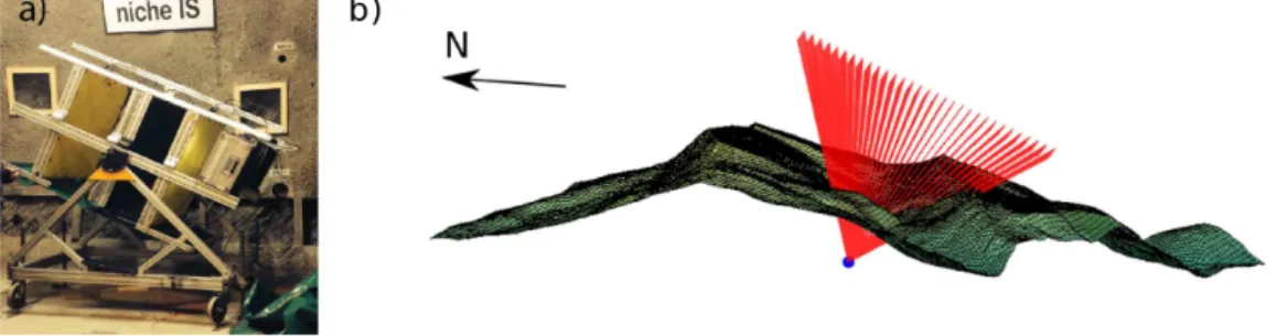
the front and rear matrices is set to 100 cm for this study (Fig. 1a). Because of the large 134
volume of rock studied compared to the detector size, we admit a point-like approximation 135
of the detector (Lesparre et al., 2010). With this approximation, given that two points are 136
sufficient to uniquely determine a direction, events whose pair of pixels in the front and the 137
rear matrices share the same relative direction are considered to correspond to the same 138
trajectory. This yields a total of (2Nx− 1) × (2Ny− 1) = 961 axes of observation studied
139
(represented in Fig. 1b). 140
The passage of muons is detected with wave-length shifting optical fibers that transport 141
the photons generated by the scintillators to the photomultiplier, where they are detected 142
based on a time coincidence logic. The optoelectronic chain has been developed from high-143
energy particle experiments on the concept of the autonomous, Ethernet-capable, low power, 144
smart sensors (Marteau et al., 2014). In order to support strenuous field conditions, besides 145
being sensitive the detector is also robust, modular and transportable (Lesparre et al., 2012). 146
In this experiment, the muon detector was deployed in the Mont Terri Underground Rock 147
Laboratory (URL) and acquired data for 382 days between October 2016 and February 148
2018. The minimum and the maximum amount of rock traversed by muons registered by 149
the detector are of approximately 200 and 500 m, respectively. Prior to the underground 150
measurements, a calibration experiment was performed by measuring the open-sky muon 151
flux at the zenith, from which we register a total acceptance of 1385 cm2 sr for our data set
152
(Lesparre et al., 2010). 153
Figure 1. a) The muon telescope deployed in the Mont Terri URL. b) Telescope’s position (blue) and axes of observation (red), along with the topography.
154 155
3 Methodology
156Our data set consists of a list of muon detections called “events”. Each event is char-157
acterized by the arrival time and the direction of the particle (possible directions shown in 158
Fig. 1b). From these data, we compute the average cosmic muon rate, R, using a 30-day 159
width Hamming moving average window (Hamming, 1998). In order to increase the signal 160
to noise ratio and, therefore, to improve the statistics in our analysis, we merge the signals 161
from all the directions together (e.g. Jourde et al., 2016). Such a merging is done exclusively 162
to compute R. 163
Seasonal variations in R, caused by the temperature changes in the atmosphere, can be treated in terms of an effective temperature (Barrett et al., 1952), Teff:
∆R hRi = αT
∆Teff
hTeffi
, (1)
where αTis the effective temperature coefficient, hRi is the mean muon rate and hTeffi is the
164
mean effective temperature. Teff is defined as the temperature of an isothermal atmosphere
165
that produces the same meson intensities as the actual atmosphere. Thus, it is related to 166
the atmosphere’s temperature profile, and it is associated to the altitudes where observed 167
muons are produced. We use the parametrization given by Grashorn et al. (2010): 168 Teff = R∞ 0 W (X)T (X)dX R∞ 0 W (X)dX , (2)
where the temperature, T (X), is measured as a function of atmospheric depth, X. The 169
weights, W (X), contain the contribution of each atmospheric depth to the overall muon 170
production. These weights depend on the threshold energy Eth, that is, the minimum
171
energy required for a muon to survive a particular opacity in order to reach the underground 172
detector. Since T (X) is measured at discrete levels of X, we perform a numerical integration 173
based on a quadratic interpolation between temperature measurements to obtain Teff.
174
The effective temperature will be different for different zenith angles. To compare Teff
175
variations to our measured muon rates, we need to account for this dependence. Following 176
Adamson et al. (2014), we bin the zenith angle distribution and calculate a weighted effective 177
temperature, Teffweight, as: 178 Teffweight= M X i=1 Fi· Teff(θi) , (3)
where M is the number of zenith-angle bins, Teff(θi) is the effective temperature in bin i
179
and Fi is the fraction of muons observed in that bin. The formula for Teff(θi) is similar
180
to Eq. (2), but the atmospheric depth is replaced by X/ cos θ and Eth is calculated for
181
each zenith angle as well. From now on, we will refer to Teffweight as Teff. These values are
182
calculated four times a day and then day-averaged, and the resulting standard deviation 183
is used as an uncertainty estimate of the effective temperature daily mean value. Thus, a 184
representative value of effective temperature is calculated for each day, which fully accounts 185
for the particular setup of our experiment. 186
The goodness of fit of the linear relationship in Eq. (1) can be quantified by the Pearson 187
correlation coefficient r. This parameter is equal to ±1 for a full positive/negative linear 188
correlation, respectively, and 0 for no correlation. We perform a linear regression between 189
the relative muon rate and effective temperature variations using Monte Carlo simulations. 190
In this way, we can account for error bars in both variables and compute the uncertainty of 191
the fitted parameters. Following Adamson et al. (2010), the intercept is fixed at zero and 192
the slope of the linear fit is the effective temperature coefficient, αT. To evaluate the effects
193
of systematic uncertainties we modify hTeffi and the parameters involved in the computation
194
of Teff(i.e. the twelve input parameters in W (X) , c.f. Adamson et al., 2010) and recalculate
195
the effective temperature coefficient, αT. These systematic errors are added in quadrature
196
to the statistical error obtained from the linear fit in orden to obtain the experimental value 197
of αT.
198
We also use Monte Carlo simulations to determine the theoretical expected value of the 199
effective temperature coefficient, αtheoryT , in order to compare it with the experimental one. 200
Muon energy, Eµ, and zenithal angle, θ, are randomly sampled from the differential muon
201
spectrum given by Gaisser et al. (2016) and corrected for altitude according to Hebbeker 202
and Timmermans (2002). Then, the muon is randomly assigned an azimuthal angle, φ, 203
according to a uniform probability distribution. The overburden opacity in the Mont Terri 204
URL is determined for each combination of (φ, θ) from our muon data set, together with the 205
corresponding Eth (Tanabashi et al., 2018). We continue the Monte Carlo sampling until
206
we obtain 10,000 successful events that satisfy Eµ> Eth, for which we compute the αtheoryT
207
distribution using the expression derived by Grashorn et al. (2010). Next, we determine the 208
value of αTtheoryand its uncertainty as the mean and standard deviation of the distribution, 209
respectively. The systematic uncertainty is the one reported by Adamson et al. (2014). 210
We look for the ocurrence of SSWs during the acquisition period using the definition 211
of a major SSW given by Charlton and Polvani (2007). A major mid-winter warming is 212
considered to occur when the zonal mean zonal wind at 60◦N and 10 hPa become easterly 213
during winter. The first day on which this condition is met is defined as the central date of 214
the warming. The zonal mean zonal wind is the average east-west (zonal) wind speed along 215
a latitude circle. To ensure that only major mid-winter warmings are identified, cases where 216
the zonal mean zonal wind does not reverse back to westerly for at least 2 weeks prior to 217
their seasonal reversal to easterly in spring are assumed to be final warmings, and as such 218
are discarded. SSWs typically manifest as a displacement or a splitting of the polar vortex 219
(Charlton & Polvani, 2007), a cyclone residing on both of the Earth’s poles that goes from 220
the mid-troposphere into the stratosphere. 221
4 Results
222Based on 382 days of data, the average daily rate of cosmic muons in the Mont Terri 223
URL is of (800 ± 10) d−1, calculated by counting all the muons detected each day no 224
matter their direction or the altitude at which they were produced. We also compute an 225
average muon rate for each axis of observation, which we use to estimate the corresponding 226
opacity values. Minimum and maximum opacities are of approximately 500 and 1500 mwe, 227
respectively, while the average opacity considering all possible directions is of (700 ± 160) 228
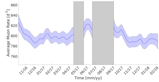
mwe. The cosmic muon rate presents significant variations in time (Fig. 2). Maximum rate 229
values occur close to the summer periods while minimum rate values occur during winter 230
times. 231
We use the ERA5 data set offered by the European Centre for Medium-range Weather 232
Forecast (ECMWF), which is a climate reanalysis data set produced using 4D-Var data 233
assimilation (Copernicus Climate Change Service (C3S), 2017). Temperature data consist 234
of interpolated (0.25◦by 0.25◦) globally gridded data on 37 atmospheric pressure levels from 235
0 to 1000 hPa, listed four times a day (00:00 h, 06:00 h, 12:00 h and 18:00 h). From this 236
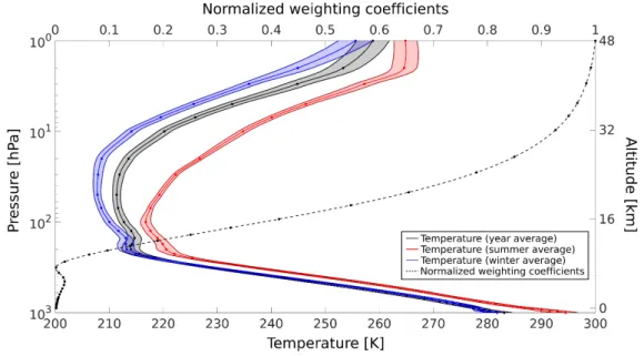
data set, we interpolate the temperature profiles at Mont Terri URL location. In Fig. 3 we 237
present the typical atmospheric temperature profiles at Mont Terri for summer, winter and 238
a year average over the analysis period. We also display in the same plot the corresponding 239
normalized weighting coefficients W as a function of pressure levels, used to compute Teff.
240
The largest temperature changes occur above ∼16 km, where the weighting coefficients are 241
more significant. The effective temperatures corresponding to the average curves and θ = 0◦ 242
are given by Teffyear= (217 ± 1) K, Tsummer
eff = (225 ± 1) K and T winter
eff = (214 ± 1) K. There
243
is thus a difference of ∼10 K between typical summer and winter conditions. 244
Figure 2. Average cosmic muon rate as a function of time, computed using a 30-day width Hamming moving average window. The colored surface delimits the 95% confidence interval. Gray bars indicate periods where the acquisition was interrupted for work in the Mont Terri URL.
245 246 247
Figure 3. Atmospheric temperature profiles (solid lines) above the Mont Terri site, and weighting coefficients (dashed line) used to calculate Teff, as a function of pressure level and altitude. The dots
represent the 37 pressure levels for which the temperature data sets are provided by the ECMWF. The right vertical axis represents approximate altitudes corresponding to the pressure levels on the left vertical axis. The summer average temperature (solid red line) and the winter average temperature (solid blue line) are computed considering a period of 1.5 months in each season during 2017. The colored surfaces represent the ±1 standard deviation in each curve. The effective temperatures of each profile are: Teffyear= (217 ± 1) K, Teffsummer= (225±1) K and Teffwinter= (214±1)
K. 248 249 250 251 252 253 254 255 256
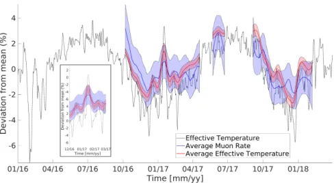
We compare the variations in the muon rate to the variations in the effective temper-257
ature in Fig. 4 in terms of relative variations (see Eq. 1). For consistency, we also apply 258
a Hamming moving average window of 30 days to the Teff time series. The two average
259
curves evolve similarly in time. Indeed, the Pearson correlation coefficient between the de-260
viation from mean of the average muon rate and that of average effective temperature yield 261
a value of 0.81. We compute a linear fit between the two data sets (see Methodology), 262
which yields an effective temperature coefficient of αT = 0.68 ± 0.03stat± 0.01syst, with
263
χ2/NDF = 414/381 being the reduced χ2 of the fit (Fig. 5). The largest contribution to
264
the systematic error in αTcomes from the ±0.06 uncertainty in the meson production ratio
265
(Barr, Robbins, Gaisser, & Stanev, 2006), the ±0.31 K uncertainty in the mean effective 266
temperature (Adamson et al., 2010) and the ±0.026 TeV uncertainty in Eth, which results
267
from the distribution of opacities along the axes of observation. To discard possible system-268
atic biases, we also performed a linear fit allowing for a non-zero y intercept. The fit resulted 269
in an estimated value of zero within one standard deviation uncertainty for this intercept, 270
and a slightly lower value of αT = 0.67 ± 0.03stat± 0.01syst for the effective temperature
271
coefficient. 272
Figure 4. Daily percent deviations from the mean of the average cosmic muon rate, the daily effective temperature, and the average effective temperature computed using a 30 days width Ham-ming moving average window. The colored surfaces delimit the 95% confidence interval associated to each curve. The inset displays a zoom around the period of time in which a major SSW is detected. 273 274 275 276 277
Figure 5. Average cosmic muon rate relative variation versus average effective temperature relative variation, fitted with a line with the y -intercept fixed at 0. The resulting slope is αT =
0.68 ± 0.03stat± 0.01systand is represented with a red line. The blue line represents the theoretical
expected value of αtheoryT = 0.65 ± 0.02stat± 0.03syst. The dotted lines represent the uncertainty
of each one of the values.
278 279 280 281 282
The theoretical expected value was found to be αtheoryT = 0.65 ± 0.02stat± 0.03syst.
283
Thus, the experimentally estimated value is consistent with the theoretical one within one 284
standard deviation. In Fig. 6 we present our estimated value of αTalong with a theoretical
model accounting for pions and kaons (Agafonova et al., 2018), and estimates from other 286
experiments. Our estimate is consistent with the one obtained by An et al. (2018) in similar 287
opacity conditions, and with the theoretical model. 288
Figure 6. Experimental values of the effective temperature coefficient as a function of hEthcos θi.
The red dot represents the present study. The continuous black line represents a theoretical model. The insert plot show the experiments performed at the underground Gran Sasso Laboratory. Figure adapted from Agafonova et al. (2018)
289 290 291 292
Taking a closer look at Fig. 4, we can see that an anomalous increase in the effective 293
temperature occurs between January and February 2017. The same anomalous behavior 294
can be observed in the muon rate (see inset in Fig. 4). We used the Charlton and Polvani 295
(2007) definition and the Modern-Era Retrospective analysis for Research and Applications, 296
Version 2 (MERRA-2), produced by the Goddard Earth Observing System Data Assimi-297
lation System (GEOS DAS) (Gelaro et al., 2017) to determine if a major SSW occurred 298
during this time period. We found that a major SSW took place during winter 2016-2017, 299
with February 1 as the central date of the warming. In a few days, it increased the zonal 300
mean temperature in the polar region by more than 20 K (Fig. 7 a). 301
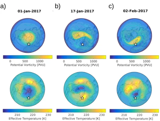
Finally, we analyzed changes produced by the SSW using Ertel’s potential vorticity 302
(Matthewman, Esler, Charlton-Perez, & Polvani, 2009). This parameter quantifies the 303
location, size, and shape of the winter polar vortex. Figure 8 shows the spatial distribution 304
of Ertel’s potential vorticity at the 850 K potential temperature surface (∼ 10 hPa, ∼ 32 305
km) for 3 different days, which are representative of the changes provoked. The figure also 306
shows the effective temperature spatial distribution during these 3 days. On January 1 (Fig. 307
8 a) the vorticity and temperature exhibit “typical” winter conditions: the polar vortex is 308
centered on the Pole, together with the minimum effective temperature. On January 17, 309
a reshaping on the polar vortex can be already observed. It is at this moment also that 310
the largest effective temperature anomaly occurs in the Mont Terri region (Fig. 8 b). On 311
February 2, that is, one day after the event can be properly classified as a major SSW 312
due to the reversal of the zonal mean zonal wind (see Fig. 7 b), the polar vortex shape is 313
still anomalous with the “comma” shaped maximum of potential vorticity now closer to the 314
Mont Terri URL (Fig. 8 c). At the same time, the effective temperature in the Mont Terri 315
region has decreased to values similar to those in January 1. 316
Figure 7. GEOS DAS MERRA-2 data used to define SSW events. a) zonal mean temperatures averaged over 60◦N-90◦N. b) zonal mean zonal wind at 60◦N. The red curve denotes values for the 2016-2017 period and the thick black curve corresponds to climatological values averaged from 1978 to 2018. The vertical blue lines reference a major SSW for that winter.
317 318 319 320
5 Discussion
326After a year of continous muon measurements with a portable muon detector under 327
relatively low-opacity conditions, we found that changes in the thermal state of the atmo-328
sphere represent the largest cause of muon rate variations. The correlation between these 329
variables was first suggested by a simple comparison of the relative variation time-series. 330
Then, it was confirmed by the large correlation coefficient (0.81), and by the fitted effec-331
tive temperature coefficient, which is in agreement with the theoretical value predicted for 332
our particular opacity and zenith angle conditions. Furthermore, our experiment was by 333
chance performed under similar opacity conditions to the Daya Bay detector, an established 334
underground muon detector especially built for neutrino experiments (An et al., 2018). Its 335
corresponding estimate of the effective temperature coefficient is also in agreement with ours 336
(Fig. 6). 337
Our muon detector is sensitive to both seasonal and short-term temperature variations. 338
The regional thermal anomaly reaching its maximum around January 17, 2017 (Fig. 4), 339
is coincident with the polar vortex changing its shape from a normal pole-centered circle 340
to a displaced “comma shaped” one (Fig. 8). This is a typical feature of a SSW (O’Neill, 341
2003). Furthermore, the criteria by Charlton and Polvani (2007) for declaring a major SSW 342
is accomplished 15 days later. The time difference can be potentially explained by the 343
zonally-averaged wind criteria used to define major SSWs, against the local character of the 344
temperature variations affecting the production of high-energy muons. 345
Under much higher opacity conditions (3,800 in mwe, i.e., more than 5 times the Mont 346
Terri URL opacity), the large muon detector of the Borexino experiment, Gran Sasso, Italy, 347
also reported muon rate variations related to this SSW in 2017 (Agostini et al., 2019). 348
Given the large opacity, most of the muons completely loose their energy before reaching 349
the detector. Thus, only high-energy muons resulting from the decay of high-energy parent 350
mesons are detected. As explained by Grashorn et al. (2010), high-energy mesons are 351
most sensitive to middle-atmosphere temperature variations due to their relatively longer 352
lifetime, and thus a higher probability of interacting with the atmosphere before decaying. 353
Figure 8. Potential vorticity at the 850 K potential temperature surface (top) and effective temperature (bottom) for January 1, January 17 and February 2, 2017, derived from the ECMWF data set. The maps are centered on the North Pole and the location of the Mont Terri Underground Laboratory (47.38◦N, 7.17◦E), close to the town of Saint-Ursanne, Switzerland, is represented with a star. 1 PVU = 10−6K m2 Kg−1 s−1. 321 322 323 324 325
This results in a higher sensitivity to temperature variations, which translates into a larger 354
effective temperature coefficient (see Fig. 6). Despite being in less advantageous conditions 355
in terms of detector acceptance and tunnel depth, our portable muon detector was also able 356
to detect these short-term effect (15-days) directly linked to middle-atmosphere dynamics 357
(Fig. 4). 358
Compared to lidar measurements, which can obtain temperature profiles over tens of 359
kilometers in altitude but have very narrow global coverage (only as wide as the laser 360
beam), muon detectors naturally provide integrated measurements in altitude, and a larger 361
horizontal coverage. Our results therefore imply that small and affordable muon detectors 362
could be used to study middle-atmosphere temperature variations without resorting to, 363
for example, expensive lidar systems. Besides being transportable, the advantage is that no 364
high-opacity conditions are needed. A minimum opacity of 50 mwe would be required to filter 365
out the temperature-dependent lowest-energy muons (Grashorn et al., 2010). Besides being 366
temperature dependent, low-energy muons can also be influenced by other phenomena such 367
as atmospheric pressure variations (Jourde et al., 2016), which is why we consider optimal to 368
remove them. However, open-sky conditions may also reveal new insights into atmospheric 369
phenomena (e.g., Hariharan et al. (2019)) and more experimental studies are needed to 370
better understand the limits of the methodology. Thus, detectors could be installed in any 371
buried facility with access to electrical power and real-time data transmission, for example 372
with a wi-fi network., such as road tunnels. In Europe, many underground research facilities 373
exist in this condition (e.g. Mont Terri UL in Switzerland, 47.4◦N; the LSBB UL in France,
374
43.9◦N; Canfranc UL in Spain, 42.7◦N). These experiments could be crucial to fill the current 375
data gap related to middle-atmospheric dynamics, in particular the study of temperature 376
anomalies associated to SSW in mid-latitudes (Sox et al., 2016). Furthermore, the technique 377
may be used to study similar phenomena in the Southern Hemisphere. 378
The effective atmospheric temperature to which the muon rate is sensitive is a weighted 379
average of a temperature profile from 0 to 50 km, with increasingly significant weights at 380
higher altitudes (Grashorn et al., 2010). Indeed, 70 % of the total weights are given between 381
50 and 26 km, 90 % between 50 and 18 km and 95 % between 50 and 15 km (see Fig. 382
3). Thus, muon rate variations are mostly sensitive to temperature variations in the high 383
stratosphere. Muon measurements can therefore complement lidar mesospheric studies (e.g., 384
Sox et al. (2016); Yuan et al. (2012)). In terms of the spatial support, in the configuration 385
used for this experiment (see Section 2), the total angular aperture of the detector is of 386
approximately ±40◦, but more than 95% of the muons are registered within an aperture of 387
±30◦. At 50 km, this represents a surface of 50×50 km2. Therefore, muon measurements
388
may be used to sample more regional atmospheric behavior. 389
Besides the potential applications to atmospheric studies, portable muon detectors may 390
be used to precisely calibrate the effective temperature curve (Fig. 6). The experimental 391
setups used to estimate these values, so far, are concentrated in either high or low-opacity 392
conditions, whereas with our approach we could sample the curve rather uniformly, even in 393
the same tunnel by varying the orientation of our detector and thus the opacity and zenith 394
angle conditions. 395
Our findings have direct implications for applications aiming to characterize density 396
variations in the subsurface (e.g. Jourde et al. (2016)). Indeed, synchronous tracking of 397
the open-sky muon rate while performing a continuous imaging of a geological body (e.g. 398
density monitoring) may not be sufficient to characterize the influence of high-atmosphere 399
temperature variations since the relative effect on the total amount of muons registered 400
increases with opacity. In turn, the mentioned possibility to improve the calibration of the 401
muon-rate dependence with middle-atmosphere dynamics will be crucial to safely remove 402
this effect. The effect will be increasingly important at higher latitudes due to the increase of 403
seasonal temperature variations, and for increasing rock opacities. At Mont Terri (47.38◦N), 404
relative effective temperature variations can be as high as 4%, which given the effective 405
temperature coefficient estimated, imply changes in muon rate as high as 3% (c.f. Fig. 4). 406
However, muon rate changes would be at maximum 1% if the opacity would be reduced by 407
one order of magnitude to 70 mwe, or equivalently 26 m of standard rock, and for vertical 408
observations. 409
Finally, relative temperature and muon rate variations are not always coincident in Fig. 410
4, despite using the same time-averaging window. Equivalently, deviations from the linear 411
relationship up to 2% and mostly around 1% can be observed in Fig. 5. The deviations from 412
a perfect correspondence are presumably due to physical phenomena influencing the muon 413
rate other than the effective atmospheric temperature. Variations arising from changes 414
in the primary cosmic rays, or changes in the geomagnetic field induced by solar wind 415
typically have temporal scales that are much smaller (e.g. seconds to hours) or much larger 416
(e.g. a solar cycle of ∼11 years). Changes reported recently as induced by lower altitude 417
atmospheric phenomena such as thunderclouds only lasted 10 minutes (Hariharan et al., 418
2019), and the low-energy muons affected by atmospheric pressure variations (Jourde et 419
al., 2016) get filtered in the first meters of rock in our experiment. A much more likely 420
explanation may be given by changes in the groundwater content of the rock overlying the 421
Mont Terri URL and will be the subject of forthcoming publications. 422
6 Conclusion
423We report for the first time sensitivity to middle-atmosphere temperature variations 424
using a portable muon detector. Changes detected are associated not only to seasonal vari-425
ations but also short-term (15-days) variations caused by a Sudden Stratospheric Warming. 426
The occurrence of this event was verified by applying a standard definition of SSWs, and 427
also observed by regional temperature and polar vortex variations obtained from ECMWF 428
and MERRA-2 reanalysis data. Previous reports on the sensitivity of muon rate to these 429
phenomena exist only for large, expensive and immobile muon detectors often times associ-430
ated to neutrino experiments and high-opacity conditions. Our findings imply that portable 431
muon detectors may be used to further study short-term temperature variations, and to 432
improve the calibration curve of muon rate dependence with an effective temperature value. 433
This, in turn, is crucial for geoscience applications aiming at studying subsurface processes 434
by characterizing density changes with muons. 435
Acknowledgments 436
This study is part of the DIAPHANE project and was financially supported by the ANR-437
14-CE 04-0001 and the MD experiment of the Mont Terri project (www.mont-terri.ch) 438
funded by Swisstopo. MRC thanks the AXA Research Fund for their financial support. 439
We are grateful to Thierry Theurillat and Senecio Schefer for their technical and logistical 440
assistance at Mont Terri URL. The MERRA data are available from https://acd-ext.gsfc 441
.nasa.gov/Data services/met/ann data.html, and the ECMWF data from https://www 442
.ecmwf.int/. Muon data used for all calculations are displayed in figures and are available 443
in the Supplementary Table S1. This is IPGP contribution number 4049. We thank the 444
editor and two anonymous reviewers for their constructive comments and suggestions, which 445
helped to improve our work. 446
References
447Abrah˜ao, T., Almazan, H., Dos Anjos, J., Appel, S., Baussan, E., Bekman, I., . . . oth-448
ers (2017). Cosmic-muon characterization and annual modulation measurement with 449
Double Chooz detectors. Journal of Cosmology and Astroparticle Physics, 2017 (02), 450
017. 451
Adamson, P., Andreopoulos, C., Arms, K., Armstrong, R., Auty, D., Ayres, D., . . . oth-452
ers (2010). Observation of muon intensity variations by season with the MINOS far 453
detector. Physical Review D , 81 (1), 012001. 454
Adamson, P., Anghel, I., Aurisano, A., Barr, G., Bishai, M., Blake, A., . . . others (2014). 455
Observation of muon intensity variations by season with the MINOS near detector. 456
Physical Review D , 90 (1), 012010. 457
Agafonova, N., Alexandrov, A., Anokhina, A., Aoki, S., Ariga, A., Ariga, T., . . . others 458
(2018). Measurement of the cosmic ray muon flux seasonal variation with the OPERA 459
detector. arXiv preprint arXiv:1810.10783 . 460
Agostini, M., Allardt, M., Bakalyarov, A., Balata, M., Barabanov, I., Barros, N., . . . oth-461
ers (2016). Flux modulations seen by the muon veto of the GERDA experiment. 462
Astroparticle Physics, 84 , 29–35. 463
Agostini, M., Altenm¨uller, K., Appel, S., Atroshchenko, V., Bagdasarian, Z., Basilico, D., 464
. . . others (2019). Modulations of the Cosmic Muon Signal in Ten Years of Borexino 465
data. Journal of Cosmology and Astroparticle Physics, 2019 (02), 046. 466
Ambrosio, M., Antolini, R., Auriemma, G., Baker, R., Baldini, A., Barbarino, G., . . . others 467
(1997). Seasonal variations in the underground muon intensity as seen by MACRO. 468
Astroparticle Physics, 7 (1-2), 109–124. 469
An, F., Balantekin, A., Band, H., Bishai, M., Blyth, S., Cao, D., . . . others (2018). Seasonal 470
variation of the underground cosmic muon flux observed at Daya Bay. Journal of 471
Cosmology and Astroparticle Physics, 2018 (01), 001. 472
Barr, G., Robbins, S., Gaisser, T., & Stanev, T. (2006). Uncertainties in atmospheric 473
neutrino fluxes. Physical Review D , 74 (9), 094009. 474
Barrett, P. H., Bollinger, L. M., Cocconi, G., Eisenberg, Y., & Greisen, K. (1952). Inter-475
pretation of cosmic-ray measurements far underground. Reviews of Modern Physics, 476
24 (3), 133. 477
Bouchta, A. (1999). Seasonal variation of the muon flux seen by AMANDA. In the proceed-478
ings of the International Cosmic Ray Conference (Vol. 2, p. 108). 479
Charlton, A. J., & Polvani, L. M. (2007). A new look at stratospheric sudden warmings. 480
Part I: Climatology and modeling benchmarks. Journal of Climate, 20 (3), 449–469. 481
Copernicus Climate Change Service (C3S). (2017). ERA5: Fifth generation of ECMWF 482
atmospheric reanalyses of the global climate. 483
Desiati, P., Tilav, S., Rocco, D., Gaisser, T., & Kuwabara, T. (2011). Seasonal variations 484
of high energy cosmic ray muons observed by the Icecube observatory as a probe of 485
kaon/pion ratio. In the proceedings of the 32nd International Cosmic Ray Conference, 486
August 11–18, Beijing, China. 487
Gaisser, T. K., Engel, R., & Resconi, E. (2016). Cosmic rays and particle physics. Cambridge 488
University Press. 489
Gelaro, R., McCarty, W., Su´arez, M. J., Todling, R., Molod, A., Takacs, L., . . . others 490
(2017). The modern-era retrospective analysis for research and applications, version 491
2 (MERRA-2). Journal of Climate, 30 (14), 5419–5454. 492
Goncharenko, L., Chau, J., Liu, H.-L., & Coster, A. (2010). Unexpected connections 493
between the stratosphere and ionosphere. Geophysical Research Letters, 37 (10). 494
Grashorn, E., De Jong, J., Goodman, M., Habig, A., Marshak, M., Mufson, S., . . . Schreiner, 495
P. (2010). The atmospheric charged kaon/pion ratio using seasonal variation methods. 496
Astroparticle Physics, 33 (3), 140–145. 497
Hamming, R. W. (1998). Digital filters. Courier Corporation. 498
Hariharan, B., Chandra, A., Dugad, S., Gupta, S., Jagadeesan, P., Jain, A., . . . others 499
(2019). Measurement of the electrical properties of a thundercloud through muon 500
imaging by the GRAPES-3 experiment. Physical Review Letters, 122 (10), 105101. 501
Hebbeker, T., & Timmermans, C. (2002). A compilation of high energy atmospheric muon 502
data at sea level. Astroparticle Physics, 18 (1), 107–127. 503
Jourde, K. (2015). Un nouvel outil pour mieux comprendre les syst`emes volcaniques: la to-504
mographie par muons, application `a la Soufri`ere de Guadeloupe (PhD Thesis). Institut 505
de Physique du Globe de Paris (IPGP). 506
Jourde, K., Gibert, D., Marteau, J., de Bremond d’Ars, J., Gardien, S., Girerd, C., & 507
Ianigro, J.-C. (2016). Monitoring temporal opacity fluctuations of large structures 508
with muon radiography: a calibration experiment using a water tower. Scientific 509
Reports, 6 , 23054. 510
Jourde, K., et al. (2016). Muon dynamic radiography of density changes induced by hy-511
drothermal activity at the La Soufri`ere of Guadeloupe volcano. Scientific Reports, 6 , 512
33406. 513
Kang, W., & Tziperman, E. (2017). More frequent sudden stratospheric warming events due 514
to enhanced MJO forcing expected in a warmer climate. Journal of Climate, 30 (21), 515
8727–8743. 516
Lesparre, N., Gibert, D., Marteau, J., D´eclais, Y., Carbone, D., & Galichet, E. (2010). 517
Geophysical muon imaging: feasibility and limits. Geophysical Journal International , 518
183 (3), 1348–1361. 519
Lesparre, N., Marteau, J., D´eclais, Y., Gibert, D., Carlus, B., Nicollin, F., & Kergosien, B. 520
(2012). Design and operation of a field telescope for cosmic ray geophysical tomogra-521
phy. Geoscientific Instrumentation, Methods and Data Systems, 1 , 33–42. 522
Limpasuvan, V., Thompson, D. W., & Hartmann, D. L. (2004). The life cycle of the 523
Northern Hemisphere sudden stratospheric warmings. Journal of Climate, 17 (13), 524
2584–2596. 525
Liu, H.-L., & Roble, R. (2002). A study of a self-generated stratospheric sudden warming 526
and its mesospheric–lower thermospheric impacts using the coupled time-gcm/ccm3. 527
Journal of Geophysical Research: Atmospheres, 107 (D23), ACL–15. 528
Marteau, J., de Bremond d’Ars, J., Gibert, D., Jourde, K., Gardien, S., Girerd, C., & 529
Ianigro, J.-C. (2014). Implementation of sub-nanosecond time-to-digital convertor in 530
field-programmable gate array: applications to time-of-flight analysis in muon radio-531
graphy. Measurement Science and Technology, 25 (3), 035101. 532
Marteau, J., de Bremond d’Ars, J., Gibert, D., Jourde, K., Ianigro, J.-C., & Carlus, B. 533
(2017). DIAPHANE: Muon tomography applied to volcanoes, civil engineering, ar-534
chaelogy. Journal of Instrumentation, 12 (02), C02008. 535
Marteau, J., Gibert, D., Lesparre, N., Nicollin, F., Noli, P., & Giacoppo, F. (2012). Muons 536
tomography applied to geosciences and volcanology. Nuclear Instruments and Methods 537
in Physics Research Section A: Accelerators, Spectrometers, Detectors and Associated 538
Equipment , 695 , 23–28. 539
Matthewman, N. J., Esler, J. G., Charlton-Perez, A. J., & Polvani, L. M. (2009). A new 540
look at stratospheric sudden warmings. Part III: Polar vortex evolution and vertical 541
structure. Journal of Climate, 22 (6), 1566–1585. 542
O’Callaghan, A., Joshi, M., Stevens, D., & Mitchell, D. (2014). The effects of different sud-543
den stratospheric warming types on the ocean. Geophysical Research Letters, 41 (21), 544
7739–7745. 545
O’Neill, A. (2003). Stratospheric sudden warmings. In J. R. Holton, J. A. Pyle, & J. A. Curry 546
(Eds.), Encyclopedia of atmospheric sciences (p. 1342-1353). Elsevier. 547
Osprey, S., Barnett, J., Smith, J., Adamson, P., Andreopoulos, C., Arms, K., . . . others 548
(2009). Sudden stratospheric warmings seen in MINOS deep underground muon data. 549
Geophysical Research Letters, 36 (5). 550
Rosas-Carbajal, M., Jourde, K., Marteau, J., Deroussi, S., Komorowski, J.-C., & Gibert, 551
D. (2017). Three-dimensional density structure of La Soufri`ere de Guadeloupe lava 552
dome from simultaneous muon radiographies and gravity data. Geophysical Research 553
Letters, 44 (13), 6743–6751. 554
Scherhag, R. (1952). Die explosionartigen Stratospharenwarmungen des Spatwinters 1951-555
1952. Ber. Deut. Wetterd., 6 , 51–63. 556
Schimanke, S., Spangehl, T., Huebener, H., & Cubasch, U. (2013). Variability and trends 557
of major stratospheric warmings in simulations under constant and increasing GHG 558
concentrations. Climate Dynamics, 40 (7-8), 1733–1747. 559
Sox, L., Wickwar, V. B., Fish, C. S., & Herron, J. P. (2016). Connection between the 560
midlatitude mesosphere and sudden stratospheric warmings as measured by Rayleigh-561
scatter lidar. Journal of Geophysical Research: Atmospheres, 121 (9), 4627–4636. 562
Tanabashi, M., et al. (2018). (Particle Data Group). Phys. Rev. D , 98 (030001). 563
Thompson, D. W., Baldwin, M. P., & Wallace, J. M. (2002). Stratospheric connection 564
to Northern Hemisphere wintertime weather: Implications for prediction. Journal of 565
Climate, 15 (12), 1421–1428. 566
Vigorito, C. F., Selvi, M., Molinario, A., Bruno, G., Trinchero, G., Fulgione, W., & Ghia, 567
P. (2017). Underground flux of atmospheric muons and its variations with 25 years of 568
data of the LVD experiment. PoS , 291. 569
Yuan, T., Thurairajah, B., She, C.-Y., Chandran, A., Collins, R., & Krueger, D. (2012). 570
Wind and temperature response of midlatitude mesopause region to the 2009 sudden 571
stratospheric warming. Journal of Geophysical Research: Atmospheres, 117 (D9). 572