HAL Id: hal-01461698
https://hal.archives-ouvertes.fr/hal-01461698
Submitted on 13 Feb 2017
HAL is a multi-disciplinary open access
archive for the deposit and dissemination of
sci-entific research documents, whether they are
pub-lished or not. The documents may come from
teaching and research institutions in France or
abroad, or from public or private research centers.
L’archive ouverte pluridisciplinaire HAL, est
destinée au dépôt et à la diffusion de documents
scientifiques de niveau recherche, publiés ou non,
émanant des établissements d’enseignement et de
recherche français ou étrangers, des laboratoires
publics ou privés.
Bayesian multifractal analysis of multi-temporal images
using smooth priors
Sébastien Combrexelle, Herwig Wendt, Jean-Yves Tourneret, Patrice Abry,
Stephen Mclaughlin
To cite this version:
Sébastien Combrexelle, Herwig Wendt, Jean-Yves Tourneret, Patrice Abry, Stephen Mclaughlin.
Bayesian multifractal analysis of multi-temporal images using smooth priors. IEEE Workshop on
statistical signal processing (SSP 2016), Jun 2016, Palma de Mallorca, Spain. pp. 1-5. �hal-01461698�
O
pen
A
rchive
T
OULOUSE
A
rchive
O
uverte (
OATAO
)
OATAO is an open access repository that collects the work of Toulouse researchers and
makes it freely available over the web where possible.
This is an author-deposited version published in :
http://oatao.univ-toulouse.fr/
Eprints ID : 17198
The contribution was presented at SSP 2016 :
http://ssp2016.tsc.uc3m.es/
To cite this version :
Combrexelle, Sébastien and Wendt, Herwig and Tourneret,
Jean-Yves and Abry, Patrice and Mclaughlin, Stephen Bayesian multifractal
analysis of multi-temporal images using smooth priors. (2016) In: IEEE
Workshop on statistical signal processing (SSP 2016), 26 June 2016 - 29 June
2016 (Palma de Mallorca, Spain).
Any correspondence concerning this service should be sent to the repository
administrator:
[email protected]
BAYESIAN MULTIFRACTAL ANALYSIS OF MULTI-TEMPORAL IMAGES USING SMOOTH
PRIORS
S. Combrexelle
1, H. Wendt
1, J.-Y. Tourneret
1, P. Abry
2, S. McLaughlin
31IRIT - ENSEEIHT, CNRS, University of Toulouse, F-31062 Toulouse, France, [email protected] 2CNRS, Physics Dept., Ecole Normale Sup´erieure de Lyon, F-69364 Lyon, France, [email protected] 3School of Engineering and Physical Sciences, Heriot-Watt University, Edinburgh, UK, [email protected]
ABSTRACT
Texture analysis can be conducted within the mathematical frame-work of multifractal analysis (MFA) via the study of the regularity fluctuations of image amplitudes. Successfully used in various ap-plications, however MFA remains limited to the independent anal-ysis of single images while, in an increasing number of applica-tions, data are multi-temporal. The present contribution addresses this limitation and introduces a Bayesian framework that enables the joint estimation of multifractal parameters for multi-temporal im-ages. It builds on a recently proposed Gaussian model for wavelet leaders parameterized by the multifractal attributes of interest. A joint Bayesian model is formulated by assigning a Gaussian prior to the second derivatives of time evolution of the multifractal attributes associated with multi-temporal images. This Gaussian prior ensures that the multifractal parameters have a smooth temporal evolution. The associated Bayesian estimators are then approximated using a Hamiltonian Monte-Carlo algorithm. The benefits of the proposed procedure are illustrated on synthetic data.
Index Terms— Multifractal Analysis, Bayesian Estimation, Texture Analysis, Multivariate image, Hamiltonian Monte Carlo
1. INTRODUCTION
Context. In image processing, texture characterization is a stan-dard problem for which different paradigms have been proposed. Multifractal analysis (MFA) is one such and characterizes a texture via the local fluctuations of the point-wise regularity of image ampli-tudes. More specifically, the texture is encoded in the so-called
mul-tifractal spectrumD(h) collecting the Hausdorff dimensions of the sets of points sharing the same local regularity, classically measured by the H¨older exponent h, cf., e.g., [1–4] and references therein. Multifractal models are deeply tied to scale invariance properties. These properties are practically assessed via the exponentsζ(q) of the power laws, over a range of scales2j, of the sample moments of
multiresolution quantitiesT (j, k) of the image X at spatial position k and scale2j S(q, j),n1 j X k |T (j, k)|q≃ (2j)ζ(q), j1≤ j ≤ j2 (1)
wherenjis the number of multiresolution quantities at scale2j. The
present work dwells on the wavelet leadersl(j, k) that have been shown to match MFA purposes [1, 4] (their definition is recalled in Section 2). These so-called scaling exponentsζ(q) are intimately linked to the multifractal spectrumD(h) via the Legendre transform
This work was supported by ANR BLANC 2011 AMATIS BS0101102. S. Combrexelle was supported by the Direction G´en´erale de l’Armement (DGA). SML acknowledges the support of EPSRC via grant EP/J015180/1.
D(h)≤ L(h) , infq∈R[2 + qh− ζ(q)]. This link enables the
prac-tical discrimination between multifractal models through the char-acterization ofζ(q). Notably, the two most prominent classes of processes used to model scale invariance in data are the self-similar processes [5], for whichζ(q) is linear in the vicinity of q = 0, and multifractal multiplicative cascade (MMC) based processes [6], as-sociated with a strictly concave functionζ(q). This discrimination can be efficiently handled via the polynomial expansion ofζ(q) (at q = 0), ζ(q) =Pm≥1cmqm/m!, by considering the coefficients
cm, termed log-cumulants [4, 7, 8]. It can be shown that the second
log-cumulantc2, referred to as intermittency or multifractality
pa-rameter, is strictly negative for multiplicative cascades whereas it is identically zero for self-similar processes, cf., e.g, [1,9]. The estima-tion ofc2is thus of paramount importance in MFA since it enables
the identification of the model that best fits the data. For more details on MFA, the reader is referred to, e.g., [1–4, 10].
Estimation of c2. The log-cumulantscmhave been shown to be
directly tied to the cumulants of the logarithm of the multiresolution quantities [7]. Specifically, for the multifractality parameterc2
C2(j), Var [ln l(j, k)] = c02+ c2ln 2j. (2)
In view of (2), the classical estimation procedure forc2is defined as
the linear regression of the sample variance dVar[·] of the log-leaders with respect to scalej
ˆ c2= 1 ln 2 j2 X j=j1 wjdVar[ln l(j, k)] (3)
wherewj are appropriate regression weights [4, 9, 11]. This
esti-mator is widely used and known to provide relatively poor perfor-mance, in particular for small image size. Different attempts to improve estimation performance are reported in the literature. A generalized method of moments has been proposed [12]. This pro-cedure relies on fully parametric models that are often too restric-tive in real-world applications. More recently, Bayesian estima-tors forc2 have been proposed [13, 14]. This approach builds on
a semi-parametric model for the multivariate statistics of the log-leaders whose variance-covariance structure is controlled by the pair (c2, c02). The resulting Gaussian likelihood is numerically evaluated
using a closed-form Whittle approximation, and the Bayesian infer-ence is accomplished by a Markov chain Monte Carlo (MCMC) al-gorithm with Metropolis-Hasting within Gibbs (MHG) moves using random walk proposals. However, these approaches are all designed for processing single images only and cannot be used to take into account the information that is potentially jointly conveyed in a col-lection of several multi-temporal images.
Goals and contributions. The goal of the present work is to in-troduce a novel Bayesian framework suitable for the joint estima-tion ofc2for image sequences. Elaborating on the statistical model
formulated for a single image in previous work [13, 14] (recalled in Section 2), this is achieved through two original key contribu-tions detailed in Section 3. First, the assumption that multifractality evolves smoothly across the collection of images is encoded via a Gaussian prior on the second derivatives of the evolution of the mul-tifractal attributes. The degree of the induced smoothness is con-trolled by hyperparameters whose estimation is also embedded in a full Bayesian model. Second, the computation of Bayesian estima-tors associated with the proposed model is achieved via an MCMC algorithm relying on a Hamiltonian Monte Carlo scheme that per-mits the efficient exploration of the non-standard conditional distri-butions in high-dimensional variable space induced by the model. The performance of the proposed estimation procedure is analyzed in Section 4 for sequences of synthetic multifractal multi-temporal images with prescribed temporal evolutions of its parameters. The results indicate that the proposed method compares very favorably against the linear regression (3) as well as with previous Bayesian formulations [13, 14].
2. STATISTICAL MODEL FOR LOG-LEADERS 2.1. Wavelet leaders
Denote χ(x) and ψ(x) a scaling function and a mother wavelet (characterized by Nψ ≥ 1 vanishing moments) defining a 1D
wavelet transform. Two-dimensional wavelets can be constructed from the tensorial products ψ(0)(x) = χ(x
1)χ(x2), ψ(1)(x) =
ψ(x1)χ(x2), ψ(2)(x) = χ(x1)ψ(x2), ψ(3)(x) = ψ(x1)ψ(x2).
Under certain admissibility conditions on φ, the collection of di-lated (to scale2j) and translated (to location x = 2jk) templates {ψ(m)j,k (x) = 2−jψ(m)(2−jx− k)} forms a basis of L2. The
dis-crete wavelet transform coefficients of an image X are defined as the inner productd(m)X (j, k) =%X, ψj,k(m)&, m = 0, . . . , 3 [15]. The
wavelet leadersl(j, k) are defined as the supremum of the wavelet modulus taken in a spatial neighborhood of2jk over all finer scales j′≤ j l(j, k), sup m∈(1,2,3),λ′⊂9λj,k |d(m)X (λ ′) | (4)
where9λj,k denotes the9 neighboring dyadic cubes of width 2j
centered around spatial location k2j, see [1, 4] for more details. 2.2. Statistical model
Recent results reported in [13, 14] suggest that the log-leaders ℓ(j, k) , ln l(j, k) can be modeled by a Gaussian random field whose covariance Cov[ℓ(j, k), ℓ(j, k + ∆k)] is approximated by a radial symmetric function parametrized by θ = [θ1, θ2]T ,
[c2, c02]T, defined as follows ̺j(∆k; θ), C2(j)−c2ln(2 jr0 j/3)+c02 ln 4 ln(1+(∆k() (∆k(≤3 c2ln((∆k(/r0j) 3 <(∆k( ≤r0j 0 r0 j<(∆k( (5) with r0
j = √nj/4. The mean of the log-leaders is linked only
to c1 and is empirically removed from the model, ¯ℓ(j, k) ,
ℓ(j, k)− %E[ℓ(j, .)], and the centered log-leaders ¯ℓ are gathered in the vector ℓj, where %E[·] is the sample mean. By assuming
moreover independence between scales, the likelihood for the vector ℓ= [ℓTj1, ..., ℓ T j2] T can be expressed as p(ℓ|θ) = j2 & j=j1 p(ℓj|θ)∝ j2 & j=j1 exp'−1 2ℓ T jΣj(θ)−1ℓj ( |Σj(θ)| 1 2 (6)
where Σj(θ) is the covariance matrix induced by ̺j,| · | denotes
the determinant andT is the transpose operator.
2.3. Whittle approximation
The direct evaluation of the likelihood (6) requires computing the covariance matrix inverses Σj(θ)−1. As proposed in [13, 14], this
can be circumvented by replacing (6) with the numerically robust and efficient Whittle approximation [16–18]
p(ℓj|θ) ∝ exp −12 X m∈Jj ln φj(m; θ)+Ij(m; ℓj) φj(m; θ) (7) that evaluates the fit between the periodogram of the log-leaders Ij(m, ℓj) and the spectral density φj(m; θ) associated with the
covariance model over the frequencies ωm = 2πm/nj with
m∈ Jj , [[⌊(−√nj− 1)/2⌋, . . . ,√nj− ⌊√nj/2⌋]]2\0. A closed-form expression of the spectral density,φj(m; θ) = θ1f1,j(m) +
θ2f2,j(m), has been derived in [14], where the functions{fi,j} do
not depend on θ, hence enabling precomputation and storage of the vectors fi,j, (fi,j(m))m∈Jj), see [14] for details. By substitution of (7) in (6), the likelihood (6) can be approximated as
p(ℓ|θ) ∝ exp
-−121T.ln φ(θ) + I(ℓ)⊘ φ(θ)/ 0
(8) where φ(θ) , θ1f1+ θ2f2, with fi , [fi,jT1, . . . , f
T i,j2] T, I(ℓ) , [(Ij1(m, ℓj1) T m∈Jj1, . . . , Ij2(m, ℓj2) T m∈Jj2] T, 1 is anM×1 vector
of ones and⊘ denotes the component-wise division operator. 3. SMOOTH BAYESIAN ESTIMATION
Based on the above model and its approximation (8), we specify a Bayesian model for a sequence of images{Xt}Mt=1.
3.1. Bayesian model
Likelihood. We write ℓt and θt , [θt1, θt2]T for the centered
log-leader and parameter vectors associated with the image Xt,
re-spectively, and use the notations L, {ℓt}M
t=1and Θ= {θ1, θ2}
with θi = {θit}Mt=1. Assuming independence between leaders of
different images, the likelihood of L is given by p(L|Θ) ∝ M & t=1 p(ℓt|θt). (9)
Priors. A smooth evolution of the parameters θtis enforced by assigning a Gaussian distribution to the second order differences of θi p(θi|ǫ2i)∝ -1 ǫ2 i 0M −1 2 exp -−2ǫ12 i (Dθi(2 0 (10) where D is the Laplacian operator. This prior models the parameters θiby a simultaneous autoregression (SAR) and has been considered
in various applications, e.g., for image deconvolution [19]. It con-strains the second derivative of parameters of interest to be small and hence promotes smoothness.
Hyperpriors. The degree of smoothing depends on the values of hyperparametersǫ2i. We adopt here a full Bayesian strategy by
non-informative Jeffreys’ priorp(ǫ2i) = (ǫ2i) −1
IR+(ǫ2i), with IR+(·) the indicator function of the set R+.
Posterior distribution. Assuming a priori independence between θ1and θ2, the Bayes’ theorem yields the following posterior
p(Θ, ǫ|L) ∝ p(L|Θ)
2
&
i=1
p(θi|ǫ2i)p(ǫ2i), ǫ, [ǫ21, ǫ22]T. (11)
Bayesian estimators. In the context of MFA, only the parameters θi are of interest. We therefore consider here the marginal
poste-rior mean estimator associated with (11), denoted MMSE (minimum mean square error estimator) and defined by
θMMSEi , E[θi|L] (12)
where the expectation is taken with respect to the marginal posterior distributionp(θi|L). Since (12) involves integrating over the
poste-rior (11), its direct computation is intractable. Instead, the inference is performed by using a Gibbs sampler (GS) generating the collec-tion of samples{Θ(k), ǫ(k)}Nmc
k=1 that are asymptotically distributed
according to (11). These samples are used in turn to approximate the marginal posterior mean estimator by
θMMSEi ≈ (Nmc− Nbi)−1 NXmc
k=Nbi+1
θ(k)i (13)
whereNbiis the length of the burn-in period [20].
3.2. Gibbs sampler
The GS considered here successively generates samples according to the conditional distributions associated with the posterior distri-butionp(Θ, ǫ|L) [20].
Multifractal parameters. It can be shown that the conditional distributionp(θi|L, θi′%=i, ǫ) is not standard. Due to the high
di-mension of θi(M≫ 1), implementing an MHG procedure (with a
random walk proposal as in [13, 14]) would yield a poor exploration of the target distribution. Instead, we resort to a Hamiltonian Monte-Carlo algorithm (HMC) [21] whose strategy is recalled in the next subsection.
Hyperparameters. The conditional distributions for hyperpa-rametersǫ2
i are inverse-gamma(IG) distributions that are easy to
sample ǫ2i|θi∼ IG(M− 1 2 , ( Dθi(2 2 ). (14) 3.3. Hamiltonian Monte-Carlo
Hamiltonian system. The HMC algorithm is a sampling scheme inspired by Hamiltonian dynamics [21]. The target distribu-tion, here p(θi|L, θi′%=i, ǫ), is associated with a potential
en-ergy E(q) = − ln p(q|L, θi′%=i, ǫ) with q , θi. Moreover
p ∈ RM auxiliary momentum variables are introduced and
as-sociated with a kinetic energyK(p) = pTp/2. The Hamiltonian
H(q, p) = E(q) + K(p) defines trajectories (q(τ ), p(τ )), in con-tinuous timeτ , with constant total energy H(q, p) via the system of equationsdqdτ = ∂H
∂p(q, p), dp
dτ =−∂H∂q(q, p) [21].
Sampling. In an HMC sampling scheme, the proposal of a candi-date is achieved through the discrete evaluation of the Hamiltonian equations. More precisely, at the iterationk of the GS, starting from the initial state q0 , θ
(k)
i and p0 ∼ N (0M, IM), the system of
Hamiltonian equations is numerically integrated for a time interval of lengthδ·L using the leap-frog method, which yields the candidate (q⋆, p⋆). This candidate is then accepted with an acceptance rate
α = min(1, ρ) with ρ = exp[H(q0, p0)− H(q⋆, p⋆)]. The
leap-frog method, detailed in Algo. 1, is composed of L steps associated with an incrementδ that is tuned during the Nbifirst iterations of
the GS such thatα∈ [0.5, 0.8]. Note that this scheme requires the computation of the derivatives of the potential energy. For the model proposed in this work, the derivatives can be calculated analytically and are given by the closed-form expression
∂E(θi) ∂θt i = 1 DTDθ i ǫ2 i 2 t +1 2 . fi⊘ φ(θt)/T.1− I(ℓt)⊘ φ(θt)/ (15) where[·]tstands for thet-th element of a vector.
Algorithm 1 Sampling scheme via HMC
1: Set q0= θ(k)i and draw p0∼N (0M, IM) 2: Leap-frog method 3: forn = 0 : L− 1 4: pn+1/2= pn− δ2 ∂E ∂qT(qn) 5: qn+1= qn+ δpn+1/2 6: pn+1= pn+1/2−δ 2 ∂E ∂qT(qn+1) 7: end for 8: Set(q⋆, p⋆) = (q L, pL) and draw u∼ U[0,1] 9: Acceptance-reject
10: Computeα = min(1, exp[H(q0, p0)− H(q⋆, p⋆)]) 11: Set θ(k+1)i = q⋆ ifu < α, otherwise θ(k+1)
i = θ
(k) i
4. NUMERICAL EXPERIMENTS
Scenario. We compare the proposed multivariate Bayesian approach (denoted as mB) to the univariate Bayesian method proposed in [13] (denoted as uB) and to the linear regression (3) (denoted as LF) by applying them to a large number of independent realizations of a sequence ofM = 100 multi-temporal images defined as 2D mul-tifractal random walks (MRWs) of size27× 27. An MRW has
multifractal properties mimicking those of Mandelbrot’s log-normal cascades, with scaling exponentsζ(q) = (H− c2)q + c2q2[22].
Typical realizations of MRW images are plotted in Fig. 1 for three different values ofc2. We use a Daubechies wavelet withNψ = 2
vanishing moments and scales(j1, j2) = (1, 3) in the analysis and
setH = 0.72. Four different evolutions of c2 across the image
sequences are studied, with values forc2 ranging from−0.04 to
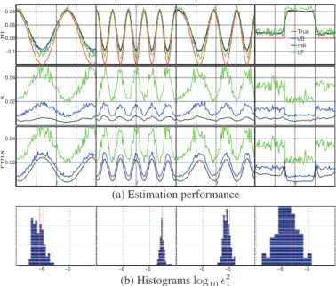
−0.12: a slow sinusoidal profile, a fast sinusoidal profile, a chirp profile including both slow and fast evolutions (as a limit benchmark case violating the slow evolution assumption) and a discontinuous evolution (cf., Fig. 2, top row, left to right columns, respectively). Estimation performance. Estimation performance is quanti-fied via the average, the standard deviation (STD) and the root mean squared error (RMSE) computed for MC = 100 indepen-dent series and defined by m = %E[ˆc2], s = ( 3Var[ˆc2])
1 2 and rms = 4(m− c2)2+ s2. Results are summarized in Fig. 2
(a) for the four different evolutions ofc2 and yield the following
conclusions. All estimators succeed in reproducing on average the prescribed values ofc2 for the smooth evolutions (i.e., they have
small bias). For the discontinuous evolution ofc2, mB provides a
smooth estimate, as expected, and hence introduces a small bias in the vicinity of the discontinuities. More importantly, however, it can
c2=−0.01 c2=−0.07 c2=−0.12
Fig. 1. Realizations of 2D MRW with different values forc2.
be observed that the proposed joint Bayesian estimator mB consis-tently yields a significant reduction of STD values as compared to LF (STD divided by up to6.5) and also to the univariate Bayesian estimator uB (STD divided by up to 2.5). This demonstrates the clear benefits of the proposed Bayesian procedure for the joint esti-mation ofc2and is also reflected in RMSE values which are, except
at the locations of discontinuities,50− 70% smaller than those of uB and LF for mB.
The observed improvements come at the price of increased yet reasonable computational time (for a sequence of100 27× 27
im-ages,∼ 8s for mB instead of ∼ 1s for LF or ∼ 3s for uB). Estimation of hyperparametersǫ2i. In order to study the
ef-fectiveness of the automatic tuning of the hyperparametersǫ2 1, Fig.
2 (b) reports histograms of MMSE estimatesǫ21 MMSE
≈ (Nmc−
Nbi)−1PNk=Nmcbi+1ǫ21 (k)
for the four different evolutions ofc2. Note
that sinceǫ2
1corresponds to the variance in the prior (10), the smaller
ǫ2
1, the smoother the solution. For the sinusoidal evolutions, the
av-erage value ofǫ2
1(indicated by a thin red line in Fig. 2 (b)) is10−6.2
and10−4.5for slow and fast evolution, respectively, thus reflecting the degree of smoothness in the evolution. For the chirp, the average value is10−5and thus sightly below that of the fast sinusoid (indeed,
stronger smoothing would introduce bias and would hence be highly penalizing). The values ofǫ2
1 for the discontinuous case are
cen-tered at10−5.8and close to the slow sinusoid case, indicating that larger bias at the two discontinuities is traded off for small variability within the segments with constantc2. These results clearly
demon-strate that the model succeeds in adjusting the hyperparameter to an appropriate smoothing level for the data.
5. CONCLUSIONS AND PERSPECTIVES
This work introduced a Bayesian procedure that enables, for the first time, the joint estimation of the multifractality parameterc2for
se-quences of multi-temporal images. Building on a recent statistical model for the multivariate statistics of log-leaders of MMC based processes, the procedure relies on two mains contributions. First, a smoothness assumption for parameter values across the collection of images was encoded via a Gaussian prior on the second deriva-tives of the multifractal attributes. The resulting Bayesian model also enables the estimation of the hyperparameters controlling the amount of smoothness. Second, to bypass the difficulties resulting from non-standard conditional distributions during the Bayesian in-ference, a Hamiltonian Monte-Carlo scheme was proposed. Closed-form expressions for the derivatives required in this scheme were obtained. Our numerical results demonstrate that the proposed pro-cedure yields excellent estimation performance and significantly im-proves over previous (univariate) formulations. Future work will in-clude the extension of the proposed approach to spatial multivariate data, i.e., the joint estimation of parameters for patches of heteroge-neous multifractal images.
m −0.1 −0.08 −0.06 −0.04 True uB mB LF s0.02 0.04 r m s 0.02 0.04 t t t t
(a) Estimation performance
−6 −5 −6 −5 −6 −5 −6 −5
(b) Histogramslog10ǫ2 1
Fig. 2. Numerical experiments: (a) estimation performance (from top to bottom: mean, STD and RMSE) assessed on 100 independent realizations for different evolutions ofc2; (b) histograms of MMSE
estimatesǫ2 1
MMSE
.
6. REFERENCES
[1] S. Jaffard, “Wavelet techniques in multifractal analysis,” in
Fractal Geometry and Applications: A Jubilee of Benoˆıt Man-delbrot, Proc. Symp. Pure Math., M. Lapidus and M. van Frankenhuijsen, Eds. 2004, vol. 72(2), pp. 91–152, AMS. [2] R. Lopes and N. Betrouni, “Fractal and multifractal analysis: A
review,” Medical Image Analysis, vol. 13, pp. 634–649, 2009. [3] J. F. Muzy, E. Bacry, and A. Arneodo, “The multifractal
for-malism revisited with wavelets,” Int. J. of Bifurcation and Chaos, vol. 4, pp. 245–302, 1994.
[4] H. Wendt, S. G. Roux, S. Jaffard, and P. Abry, “Wavelet lead-ers and bootstrap for multifractal analysis of images,” Signal
Proces., vol. 89, no. 6, pp. 1100 – 1114, 2009.
[5] B. B. Mandelbrot and J. W. van Ness, “Fractional Brownian motion, fractional noises and applications,” SIAM Review, vol. 10, pp. 422–437, 1968.
[6] B. B. Mandelbrot, “A multifractal walk down Wall Street,” Sci.
Am., vol. 280, no. 2, pp. 70–73, 1999.
[7] B. Castaing, Y. Gagne, and M. Marchand, “Log-similarity for turbulent flows,” Physica D, vol. 68, no. 3-4, pp. 387–400, 1993.
[8] H. Wendt, S. Jaffard, and P. Abry, “Multifractal analysis of self-similar processes,” in Proc. IEEE Workshop Statistical
Signal Proces. (SSP), Ann Arbor, USA, 2012.
[9] H. Wendt, P. Abry, and S. Jaffard, “Bootstrap for empirical multifractal analysis,” IEEE Signal Proces. Mag., vol. 24, no. 4, pp. 38–48, 2007.
[10] R. H. Riedi, “Multifractal processes,” in Theory and
applica-tions of long range dependence, P. Doukhan, G. Oppenheim, and M.S. Taqqu, Eds. 2003, pp. 625–717, Birkh¨auser.
[11] P. Abry, R. Baraniuk, P. Flandrin, R. Riedi, and D. Veitch, “Multiscale nature of network traffic,” IEEE Signal Proces.
Mag., vol. 19, no. 3, pp. 28–46, 2002.
[12] T. Lux, “Higher dimensional multifractal processes: A GMM approach,” J. Business Econ. Stat., vol. 26, pp. 194–210, 2007. [13] S. Combrexelle, H. Wendt, N. Dobigeon, J.-Y. Tourneret, S. McLaughlin, and P. Abry, “Bayesian estimation of the multi-fractality parameter for image texture using a Whittle approxi-mation,” IEEE T. Image Proces., vol. 24, no. 8, pp. 2540–2551, 2015.
[14] S. Combrexelle, H. Wendt, J.-Y. Tourneret, P. Abry, and S. McLaughlin, “Bayesian estimation of the multifractality pa-rameter for images via a closed-form Whittle likelihood,” in
Proc. 23rd European Signal Proces. Conf. (EUSIPCO), Nice, France, 2015.
[15] S. Mallat, A Wavelet Tour of Signal Processing, Academic Press, 3rd edition, 2008.
[16] P. Whittle, “On stationary processes in the plane,” Biometrika, vol. 41, pp. 434–449, 1954.
[17] M. Fuentese, “Approximate likelihood for large irregularly spaced spatial data,” J. Am. Statist. Assoc., vol. 102, pp. 321– 331, 2007.
[18] V. V. Anh and K. E. Lunney, “Parameter estimation of random fields with long-range dependence,” Math. Comput. Model., vol. 21, no. 9, pp. 67–77, 1995.
[19] P. Campisi and K. Egiazarian, Blind image deconvolution:
the-ory and applications, CRC press, 2007.
[20] C. P. Robert and G. Casella, Monte Carlo Statistical Methods, Springer, New York, USA, 2005.
[21] R. M. Neal, “MCMC using Hamiltonian dynamics,”
Hand-book of Markov Chain Monte Carlo, vol. 54, pp. 113–162, 2010.
[22] R. Robert and V. Vargas, “Gaussian multiplicative chaos revis-ited,” Ann. Proba., vol. 38, no. 2, pp. 605–631, 2010.