Calculating failure probabilities of passive systems during transients

CALCULATING FAILURE PROBABILITIES OF PASSIVE

SYSTEMS DURING TRANSIENTS

By

Francisco J. Mackay

Electronics Engineer

Academia Politecnica Naval, Chile - 2001

SUBMITTED TO THE DEPARTMENT OF NUCLEAR SCIENCE AND

ENGINEERING IN PARTIAL

FULFILLMENT OF THE REQUIREMENTS FOR THE DEGREE OF

MASTER OF SCIENCE IN NUCLEAR SCIENCE AND ENGINEERING

AT THE

MASSACHUSETTS INSTITUTE OF TECHNOLOGY

JANUARY 2007

@2007

Massachusetts Institute ofTechnology.

All

rights reserved.

The author hereby grants to MIT permission to reproduce

and to distribute publicly paper and electronic

copies of this thesis documert ip whole or in part

in any medium now known

t

ereafter created.

Signature of the author: ___

Departmei-oNuclear Sciennce

e

oogy

YL~afu

Ja u ry

0

Certified by:

.

.,

George E. Apostolakis

Professor of Nuclear Science and Engineering

Thesis supervisor

Accepted by:

.

..

-Ab

_{Pavel Hejzlar}

.

PrinciRal Research Scientist

Accepted by:

OCT 1

2

2007

LIBRARIES

I

Jeffrey A. Coderre

Associate Professor of Nuclear Science and Engineering

Chairman, Department Committee on Graduate Students

CALCULATING FAILURE PROBABILITIES OF PASSIVE

SYSTEMS DURING TRANSIENTS

by

Francisco J. Mackay

Submitted to the Department of Nuclear Science &

Engineering on January 23, 2007 in partial fulfillment of

the requirements for the Degree of Master of Science in

Nuclear Science and Engineering

1. ABSTRACT

A time-dependent reliability evaluation of a two-loop passive Decay Heat

Removal (DHR) system was performed as part of the iterative design process for a

helium-cooled fast reactor. The system was modeled using RELAP5-3D. The

uncertainties in input parameters were assessed and were propagated through the model

using Latin Hypercube Sampling. An important finding was the discovery that the

smaller pressure loss through the DHR heat exchanger than through the core would make

the flow to bypass the core through one DHR loop, if two loops operated in parallel.

This finding is a warning against modeling only one lumped DHR loop and assuming that

n of them will remove n times the decay power. Sensitivity analyses revealed that there

are values of some input parameters for which failures are very unlikely. The calculated

conditional (i.e., given the LOCA) failure probability was deemed to be too high leading

to the identification of several design changes to improve system reliability. This study is

an example of the kinds of insights that can be obtained by including a reliability

assessment in the design process. It is different from the usual use of PSA in design,

which compares different system configurations, because it focuses on the

thermal-hydraulic performance of a safety function.

Thesis supervisor: George E. Apostolakis

2. ACKNOWLEDGMENT

I want to thank my wife for, without her support and care, this work could not

have been possible. To Prof. George E. Apostolakis, for his guidance, support, counsel

and for the most his patience. To Pavel Hejzlar, whose knowledge was always an

incredible source of light when walking through the dark paths of accurate simulation.

To Prof. Michael J. Driscoll, for being an unlimited source of ideas and support through

the whole process. Last, but not least, to Chris Handwerk, Mike Stawicki, David

Carpenter, Tyler Ellis, Giovanbattista Patalano, Edoardo Cavalieri, Lorene Debesse and

Rodney Busquim for their friendship and willingness to help me in so many ways. This

3. TABLE OF CONTENTS

A B ST R A C T ...

... . . . . 3

A C K N O W LED G M EN T ...

... 4

TABLE OF CONTENTS ...

... 5

TA BLE OF FIG U R ES...6

INTRODUCTION...

...

7

SYSTEM DESCRIPTION...13

A N A L Y S IS ...

19

7.1.

Mechanistic Model ...

...

.

... 19

7 .2 .

U n certain ties ...

24

7.3.

Uncertainty Propagation ...

... 27

7.4.

Failure Criteria ...

28

7.5.

System Failure Criteria ...

29

7 .6 .

R esu lts...

... ...

... 3 0

RISK-BASED DESIGN CHANGES ...

41

C O N C LU SIO N S ...

43

. R EFEREN C ES ...

. . . . ..

...

... 45

S APPENDICES ...

...

47

11.1.

APPENDIX A: RELAP5-3D NODALIZATION DIAGRAM ... 47

11.2.

APPENDIX B: RELAP5-3D NOMINAL INPUT DECK ... 48

11.3.

APPENDIX C: TABLE OF PROPAGATED UNCERTAITY...157

11.4.

APPENDIX D: UTILIZED ALGORITHMS ...

163

8.

9.

10

4. TABLE OF FIGURES

Figure 1. An example of load and capacity stochastic processes...8

Figure 2. Schem atic GFR system layout ...

13

Figure 3. Schematic of a natural circulation loop ...

15

Figure 4. RELAP5-3D Nodalization diagram of the system...19

Figure

5.

Possible flow patterns ...

23

Figure 6 Example of the output from an LHS uncertainty propagation...28

Figure

7

M ultiple Failure Criteria...30

Figure 8 Realizations for Maximum Temperature in the Cladding...31

Figure 9 Realizations for the Maximum Temperature in the Hot Leg of DHR Loops ....33

Figure 10 Leakage Threshold Effect (cladding failure) ...

34

Figure 11 Maximum leakage and HTCS Threshold Effect (structural failure)...36

Figure 12 Search for threshold effects (Failure Mode 1, cladding failure) ... 37

5. INTRODUCTION

According to the International Atomic Energy Agency (IAEA) definition, a

passive system is either a system that is composed of passive components and structures

or a system that uses active components in a very limited way to initiate subsequent

passive operation (IAEA, 1991). Of great importance are thermal-hydraulic systems

(T-H) that fall under IAEA Categories B and C. These are characterized by moving working

fluids either without or with moving mechanical parts, such as check or relief valves,

respectively.

Passive system reliability analysis has attracted increasing attention over the last

decade. The expectation that the overall plant reliability should increase by replacing

certain active systems with passive ones is based on the fact that unreliability of active

systems is due primarily to the unreliability of the energy source that is required for them

to perform. Passive system functionality does not rely on an external source of energy,

but on an intelligent use of the naturally available one (gravity), which is always present.

As the research in the field advances, the tradeoffs between passive and active systems

are becoming clear. Although the energy source is always available for a passive system,

it is normally weak. As a result, passive systems are much more sensitive to changes in

the surroundings than active ones (Pagani et al, 2005). In addition, the operators cannot

control passive systems the way they can control the performance of active systems.

Since the reliability evaluation does not depend on the availability of the driving

energy, a new description of the concept of failure is required. The concept of passive

(2003). It describes "failure" in terms of a "load" exerted during the perfornnance of the

system on its components and the "capacity" of these components to withstand that load.

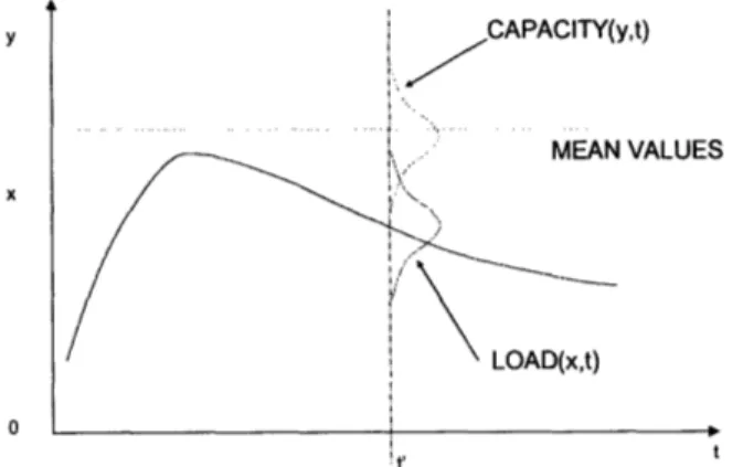
An example of a load is the temperature at a certain point as the system operates. The

temperature limit of the material at that point above which damage occurs is the capacity

of the system. In general, both the load and the capacity are uncertain and may depend

on time (an example is shown in Figure 1). The probability that the load exceeds the

capacity is the failure probability of the system for that point in time. Two models are

therefore needed, one for the load and one for the capacity. In general, the capacity

model may be correlated with the load model. In other words, the capacity of a

component can be a function of its state and therefore time-dependent. An example of

this is the dependence of material yield stress on temperature. Therefore, if the analyzed

component is a pipe, the pressure required to break it is a function of the temperature,

which may vary according to the performance of the system.

y X CAPACITY(y,t) ... MEAN VALUES LOAD(x,t)

Figure 1. An example of load and capacity stochastic processes.

The following tasks need to be performed to evaluate the reliability of a passive

1. Identification of the components (points in the system) where failure may occur

and their respective loads and capacities. A component may fail in a number of

ways. Failure Modes and Effects Analysis (FMEA) and Hazard and Operability

HAZOP Analysis are methods that are helpful in identifying component failure

modes (Burgazzi, 2004).

2. Definition of component failure criteria, i.e., the type of capacity model that

should be used for each load determined in the previous task. Capacity models

may be in the form of deterministic limits (e.g., imposed by a regulatory

authority) or probability distributions based on experiments and/or expert

opinions.

3. Selection of sets of parameters (boundary conditions, system properties and initial

conditions) that affect the behavior of each load determined in Task 1. The

Analytical Hierarchy Process (AHP) has been proposed to help identify these

important driving parameters (Zio et al, 2003; Marques et al, 2005).

4. Development of a probability distribution for each parameter input to the model to

represent the relevant uncertainties. This is a crucial step and is normally done

based on experiments or expert opinions (Jafari et al, 2003; Marques et al, 2005;

Pagani et al, 2005).

5.

Propagation of the uncertainty distributions of the input parameters through the

models. Many techniques have been proposed to perform this step. They range

surfaces. A discussion on the advantages and disadvantages of each option is

presented by Marques et al. (2005).

6. Calculation of system reliability. The system is considered failed if one or more

of the failure criteria are met. This means that more than one component may fail

for the same system realization (Marques et al, 2005). The result of this

calculation is the probability of failure of the system.

These tasks provide the main structure of any passive system reliability

calculation. The list does not include tasks aimed at improving the quality and efficiency

of the calculations, such as early sensitivity analyses or iteration loops between tasks. A

more detailed description of these tasks is presented in (Jafari et al, 2003; Marques et al,

2005).

This work presents a detailed description of the time-dependent reliability

evaluation of a passive decay heat removal system after a Lost-of-Coolant-Accident

(LOCA). We emphasize the difficulties found in the process, propose solutions, and

describe the lessons learned regarding the design itself. Our focus is on uncertainties and

their propagation.

A preliminary design of a helium-cooled fast reactor constitutes the case study. It

is part of the MIT studies on a Gas-cooled Fast Reactor (GFR) design. The system and

its components were simulated using RELAP5-3D (INEEL, 2001). The entire system

operates as one passive system whose initiation is triggered by the reactor scram after a

The complete description of the reliability calculation is presented in Section 3,

where suggestions for design improvement are also given by identifying the input

parameters that are driving the failure of the system. Finally, conclusions on different

6. SYSTEM DESCRIPTION

The GFR design considered consists of a 600 MWth helium-cooled fast reactor

core inside the Pressure Vessel (PV), a Brayton power cycle within the Power

Conversion Unit (PCU), and two 50% Decay Heat Removal (DHR) loops (Figure 2).

The core is designed to have very low pressure drop to maximize the natural circulation

capability. Moreover, the PV, the PCU and the DHR loops are surrounded by a guard

containment with a high design pressure of 2 MPa (20 bars), so that, after primary system

depressurization, the final pressure in the guard containment would be high enough to

make DHR by natural circulation of helium possible. Each DHR loop is designed to

extract 2% of the reactor nominal power (12 MWth) at a backup pressure of 1.3 MPa.

QteafEmhgnpr

Figure 2. Schematic GFR system layout.

Each DHR loop consists of two separate circuits. The first is connected to the PV

through a coaxial pipe with the cold leg running in the outside. Heat is subsequently

loop delivers the heat to a pool outside the containment building. Check valves are

placed in the cold leg of the helium section of each DHR loop. The PCU contains a

Brayton power cycle with recuperator, precooler and intercooler. The shaft that is

propelled by the turbine provides energy to the generator and to the low and high

pressure compressors of the cycle as well. More details on the GFR system layout are in

Hejzlar et al. (2005).

As will be seen later, there are several parameters that are of importance for a

natural circulation loop to work properly. An intuitive review of the phenomenon gives a

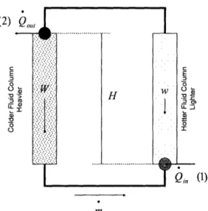
good insight into the system's dynamics. Figure 3 shows a generic loop that is the

starting point of the discussion. Heat is inserted at point (1) and extracted at point (2).

There is no heat transfer at any other point in the circuit. When the fluid is heated at

point (1) its density decreases and it begins to flow up and forms the hotter fluid column

that is shown in the figure. At the same time, when heat is extracted at point (2), the

density of the fluid increases and as a result it moves down forming the colder fluid

column shown in the figure. The difference in weight (W-w) between the two columns is

the driving force that results in a certain mass flow running through the loop. The mass

flow is primarily determined by the driving force and the resistance that the system exerts

to the flow through pipes and fittings. To increase the mass flow then one can increase

H, the difference in altitude between points (1) and (2), increase the temperature

difference between the columns, or replace the fluid by one whose density change per

(2) C

E

D

Figure 3. Schematic of a natural circulation loop.

Assuming the loop is at steady state (which implies Qo,,

-

= 0), the rate at

which the system is extracting heat from the source is equal to

Q,,

[J/s]:

Q,,,

m* Cp

*

AT

(1)

where

m

=

pVA

=

Mass Flow [kg/s]

Cp = Isobaric Heat Capacity [J/kg K]

AT = Temperature Difference between hot and cold legs [K]

p

=

Density [kg/m']

V

=

Velocity [m/s]

A

=

Flowing Area [m2]

Therefore, in order to extract more heat either the mass flow or the temperature

difference needs to be increased in the passive loop. Increasing the mass flow is

normally preferable because to increase AT almost always means to increase the

limit. Embedded in this short argument is the importance of the backup pressure. A

greater pressure means higher density of the helium and a higher mass flow through the

heat exchanger for the same fluid velocity, letting the system extract more heat from the

source, while keeping AT constant. Although not mentioned in the discussion above, an

increase in the density is also beneficial to the natural circulation phenomenon because it

reduces the friction factor along the loop due to reduced kinematic viscosity, therefore

allowing a larger mass flow.

A LOCA on the cold leg of the PCU was chosen as the initiating event of the

analysis. The system is designed to survive a 500 cm

_{break, but it was evaluated for a}

₅

cm

_{break that is much more probable (frequency: 10}

_{per year) than a large break. The}

sequence of events is as follows:

1. The cooling function is performed by the helium coming from the PCU

from the moment of the accident until the shaft with turbine and

compressors stops. During that time the flow coming out from the PCU is

divided into two streams at the point of the rupture: the first one goes

directly to the containment through the break and the second follows its

initial path to the core through the downcomer. How long the shaft runs is

a function of the size of the break. For a 500 cm

break, the Brayton cycle

would work as such, propelled by the decay heat, for a period of time

ranging between 30 to 40 minutes. This gives enough time for the decay

heat to fall below the 2% nominal power threshold, so the DHR loops can

break. The shaft stops after approximately 10 minutes. The higher

density of the helium, sustained in time because of the small break area,

plus a smaller temperature difference across the core provide more

resistance to compressors and less energy is extracted by the turbine from

helium, therefore the reduction in shaft coastdown time. During this

period the PCU is cooling down the core and the check valves placed on

the cold legs of the natural circulation DHR loops are closed.

2. Once the shaft stops, the pressure difference is reversed and the check

valves open, allowing the natural circulation through the DHR loops to

start. Two parameters are important here: the pressure inside the PV and

DHR loop and the amount of decay heat that is being released at that

moment. For the case of a 500 cm

_{break, the pressure inside the PV is}

already equalized to that of the containment and the decay heat is below

the 2% nominal power threshold. Problems could arise, for example, if

the structures in the containment absorbed an excessive amount of heat,

therefore reducing the backup pressure required for natural circulation, or

if the shaft stopped when the decay heat was greater than 12 MWth. For

the

5

cm

_{break, the dynamics are different. The shaft stops within 10}

minutes of the accident but the pressure inside the PV remains high

enough to sustain a natural circulation capable to extract the decay heat

that is being produced. Nevertheless, when natural circulation through the

DHR loops starts, the temperature difference across the core is not

temperature begins to rise until it reaches its operating condition.

Meanwhile, the natural circulation is continually deteriorating by the

depressurization process that will eventually end about 30 to 40 minutes

after the accident. After that time the decay heat is below the 12 MWth

mark and, if the backup pressure is by then adequate and decaying slower

7. ANALYSIS

7. 1.Mechanistic Model

The mechanistic model simulates the dynamic behavior of the system given a set

of boundary and initial conditions and system physical properties (i.e., it is the "model of

the world" in PRA terminology (Apostolakis, 1994)). This model will be used to perform

sensitivity analyses and to propagate the uncertainties in the input parameters.

A complete model of the system was built using RELAP5-3D (INEEL, 2001).

RELAP5-3D is a thermal-hydraulic code developed by Idaho National Laboratory for the

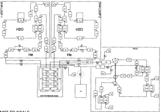
analysis of accidents in nuclear power plants. Figure 4 shows the nodalization of the

model of the system.

INU I I U Ly- daL

The DHR loops are on the top left area of the diagram and show the water and

helium sides connected together by heat exchangers. Heat exchangers are represented by

rectangles enclosing the volumes involved in the heat transfer balance. The reactor is

immediately below the DHR loops. Two long vertical volumes represent the downcomer

and, in the center of the core, two channels can be distinguished between the lower and

upper plenums; one representing the average and the other the hottest channels in the

core. On the lower right-hand corner, the PCU is modeled. The turbine and both

high-and low-pressure compressors are connected to the same shaft. There are three heat

exchangers in this part of the model and they correspond to the recuperator, the

pre-cooler and the interpre-cooler. Finally, enclosed by a dashed line circle is the valve that

simulates the rupture generating the LOCA. This valve connects the outlet of the cold leg

of the PCU to the volume that represents the containment building.

The following is a list of modeling information relevant to the results:

1. The ANS 79 Decay Heat Model is used (ANS, 1979)

2. All pipe walls are modeled for pipes in each DHR loop. The importance of

this practice comes from the fact that the heat capacity of steel is greater than

that of helium. A significant amount of mass flow is required then to either

heat them up or cool them down, therefore affecting the transient behavior of

the natural circulation loops (Hejzlar et al, 2005).

3. The core is modeled by two channels: an average and a hot one. The hot

channel simulates the hottest channel in the core in accordance to the core's

cladding and fuel. This configuration allows the monitoring of the highest

temperature in both fuel and cladding.

4. RELAP5-3D does not allow negative angular velocity for shafts and

compressor operation at negligibly small flows. To overcome this issue and

continue with calculations beyond this point, as soon as the mass flow

entering the PCU becomes smaller than 0.5% of the nominal flow, the PCU is

isolated from the rest of the system and an auxiliary external flow is injected

into it to keep the shaft running with positive angular velocity, while the rest

of the simulation is carried on in parallel. This action prevents simulation of

the effect of bypass flow through the PCU on core cooling; hence the failure

probabilities reported here are optimistic assuming that PCU can be isolated

with 100% reliability.

5. Leakage of the check valves in the DHR loops is simulated with a

dependent junction running parallel to the respective check valve. A

time-dependent junction allows the implementation of a constant negative mass

flow rate through the loop, if the pressure drop across the check valve is

positive. Otherwise, the mass flow rate is zero.

6. The heat transfer from the water loop to the pool outside the containment

building is simulated with a natural convection boundary condition with a

fixed T (bulk temperature of the pool) equal to the ambient temperature.

7. Three heat structures simulating the containment liner, the concrete on the

containment hydrodynamic volume. Their effect is important because they

absorb heat reducing the temperature of the helium in the containment and

thus the backup pressure.

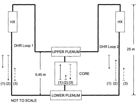
During the mechanistic analysis, several unexpected effects were discovered. The

system was initially designed with two

50%

DHR loops that would work in parallel (see

flow pattern (1) in Figure

5).

This feature needed to be changed because the check valves

of one of the DHR loops would never be open at the same time except for short periods

of unstable flow. The reason for this behavior is the smaller pressure drop through the

DHR heat exchangers than through the core and flow tendency to bypass the core through

one of the DHR loops closing check valve on this loop. Thus, if both valves are forced to

open, one of the loops would finally work backwards (see flow pattern (2), Loop 2, in

Figure

5);

stealing the mass flow from the core so that most of the flow from the correctly

operating loop proceeds through the common lower plenum to the other loop and

ultimately to the upper plenum. Such core bypass reduces substantially core flow rate

and rapidly leads to fuel overheating. To overcome this problem, the design was

modified to increase the original 2x50% capacity to 2x100% capacity DHR loops.

Furthermore, the appearance of this phenomenon clearly emphasizes the importance of

modeling the DHR loops separately instead of lumping them up into one loop that

I

(1)

25 m

3)

DINJ I I U •vL.,,•LC

Figure 5. Possible flow patterns.

Another interesting phenomenon happens if the check valves are forced to open

before the mass flow that is injected by the compressors on mounted on the coasting

down shaft stops. In this case, both loops would work backwards (see flow pattern (3) in

Figure

5)

because the pressure in the upper plenum would be smaller than that in the

lower plenum. This unintended behavior is stable at least for the decay heat levels that

occur during the first three hours after the accident. The same phenomenon is observed if

there is a leaky check valve. During normal operation the pressure difference across the

core produces a continuous flow through the leaking check valves. If the leakage of the

check valves is sufficiently high, the continuous leak forces the flow through the

emergency heat exchangers where it experiences cooling and the originally hot riser

the shaft stops, both loops continue in reversed operation mode and the sum of leaking

flows is not sufficient to cool the core thus leading to failure.

As discussed earlier, the heat absorption from the structures inside the

containment building was expected to have an impact on the evolution of its pressure and

therefore on the backup pressure once the PV and the containment pressures are

equalized. The results from a sensitivity analysis on this parameter showed that the liner

needed to be isolated and the free volume to be reduced.

After these changes to the design, the model is ready for the next stage on the

analysis: uncertainty analysis.

7.2. Uncertainties

As stated in the introduction, passive systems are sensitive to changes in the

boundary and initial conditions and to changes in the numerical values of the parameters

that define the system properties. All these conditions and parameters are called input

parameters. This sensitivity is due primarily to the weakness and uncontrollability of the

driving force, gravity.

A set of six input parameters were selected to be propagated through the model.

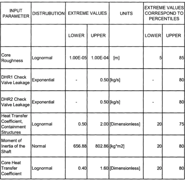
Table 1 shows these parameters and their probability distribution functions. The

selection was made based on sensitivity analyses done on several parameters and expert

INPUT EXTREME VALUES

PARAMETER DISTRUBUTION EXTREME VALUES UNITS CORRESPOND TO

PARAM ETERPECNLS _PERCENTILES

LOWER UPPER LOWER UPPER

Core_{Roughness Lognormal}

1.00E-05 1.00E-04 [m] 5 85

Roughness

DHR1 Check

Valve Leakage Exponential - 0.50 [kg/s] 80

Valve Leakage

Coefficient, Lognormal 0.50 2.00 [Dimensionless] 20 75 Containment

Structures Moment of

Inertia of the Normal 656.88 802.86 [kg*m2] 20 80

Shaft Core Heat

Transfer Lognormal 0.40 1.60 [Dimensionless] 20 80

Coefficient

Table 1 Selected Input Parameters and their probability distributions

Roughness in the Core refers to the roughness of the surfaces in the core that are

in contact with helium. Even though it is small in absolute terms, the pressure drop in the

core accounts for about 70% of the overall pressure drop along the DHR loops under

nominal operation. An increase in the roughness translates into a larger pressure drop in

decreases, the required temperature difference across the core increases for the same

amount of heat removal.

Check Valve Leakage: The first assumption is that the check valves are always

leaking. The effect of leakage is to delay the opening the valves. A backward flow

through the DHR loops is present during normal operation and during the time the PCU

is cooling the core after the accident, therefore the system has to overcome the inertia of

that flow in order to open the check valves once the PCU has stopped.

Heat Transfer Coefficient of Structures in the Containment Building (HTCS): The

result of having a greater HTCS is that blown down helium in the containment is cooled

down faster and therefore reducing the pressure that at the same point in time the

containment would have had under adiabatic conditions. Since this is a preliminary

design, the containment layout and geometry and positions of internal structures inside

are not known. Each modeled structure corresponds to the lumping of several objects

and each of these would have its own time-dependent heat transfer coefficient, so the

modeled HTCS correspond to average values. Furthermore, RELAP5-3D calculates the

heat transfer coefficient for each structure in the containment volume according to its

respective boundary condition, so the uncertainty is represented by a multiplicative factor

that modifies the HTCS calculated by the code.

Heat Transfer Coefficient in the Core (HTCC): The effect of a smaller heat

transfer coefficient is that a greater temperature gradient across the core would be

required in order to remove the same amount of heat. In this case, there is uncertainty in

heat transfer coefficient under low-Reynolds number, high heat-flux flows where local

buoyancy and acceleration forces can significantly reduce heat transfer coefficient (Lee

and Hejzlar, 2006). The uncertainty is represented by a multiplicative factor that

modifies the HTCC calculated by the code.

Moment oflnertia of the Shaft: A shaft with a greater moment of inertia is more

difficult to decelerate and therefore could run longer. This is important because as the

coastdown time is increased, the moment at which the DHR loops are initiated is also

increased placing the system in a safer operating condition with a smaller decay heat.

7.3. Uncertainty Propagation

Monte Carlo simulation is used to propagate the uncertainties in the input

parameters through the model. In order to reduce the number of trials, Latin Hypercube

Sampling (LHS) was employed. In short, this technique divides the six-dimensional

probability defined by the input parameters into a set of equiprobable six-dimensional

cubes (hypercubes) from which the samples are then chosen. The fundamental

assumption of the method is that the input variables are independent. Since only one

sample point is chosen from each hypercube, the sample points are equiprobable. More

information on LHS can be found in Helton and Davis (2003).

Once the sample is chosen, a RELAP5-3D simulation is made for each unique set

of sample points (one from each hypercube). Each set defines a scenario. Since these

sets are equiprobable, the corresponding results of RELAP5-3D are also equiprobable. A

three-hour time span starting at the moment of the accident was chosen as the simulation

pressure in the containment becomes equal to the pressure in the PV (consequently, the

flow through the rupture is negligible) after two hours. The pressure rate of change

inside the containment was never less than -17 Pa/s at the end of three hours. The

sensitivity analyses also showed that the temperature gradient at the same point was

never less than -9.0x 10

K. Furthermore, the power that is being generated at the core by

then is about 6.8 MWth, well below the design specifications of the DHR loops. For the

present work, it is assumed that the containment has no leakage.

7.4. Failure Criteria

After the simulations are finished, a screening of the output parameters is again

required in order to define which of them are going to be considered for the unreliability

evaluation. It is important to do so because new failure modes may be discovered in the

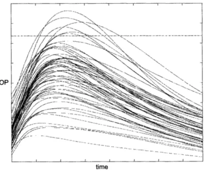
process. Figure 6 shows an example (not an actual result) for an output parameter. Each

curve corresponds to a particular scenario (set of sample points).

OP

time

The next step is to define the failure criterion for each selected output parameter.

In traditional reliability assessments, this task is done much earlier in the process and in

fact it can be made during the mechanistic analysis, after structuring the set of potentially

relevant output parameters, but it must be reviewed here because new failure modes may

have been discovered. The failure criteria used in this work are deterministic limits such

as the horizontal dashed line shown in Figure 6. Any realization that exceeds the limit is

considered a failure. Since all realizations are equally likely, the probability of failure

during the time span of the graph is equal to the number of curves that exceed the limit

divided by the total number of curves.

To write this down more formally, let A(i) be a binary variable that is equal to

unity when the

scenario (realization) leads to failure and equal to zero otherwise.

Then, the probability of failure is:

M

XA(i)

PF

M

_M

(2)

where M is the total number of realizations.

7.5. System Failure Criteria

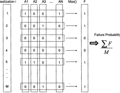
Multiple failure criteria should be used whenever more than one output parameter

may lead to failure. This means that a specific scenario may lead to no failure or at least

Let

AI,

be the failure vectors associated to N failure modes over M

realizations. Define F(i)

=

max(A, (i), A

(i),...,

(i)) Vi e {1,2,3,...,M}, then the mean

probability of multiple failure PF is define as:

M

IF(i)

PFI,-

M

₍₃₎

Figure 7 shows an example of this procedure.

Realization i 1 2 3 4 5 M Al A2 A3 ... AN Max() F 1 1 0 Failure Probability

M

Figure 7 Multiple Failure Criteria

7.6.

Results

After reviewing the parameters of the system at various points, two failure modes

were finally selected for the reliability evaluation of the system: Cladding damage in the

hot channel and structural failure in the hot legs of the DHR Loops. A limit of 1600 °C

(1873 K) was set as the maximum temperature for cladding damage. It is assumed that

the silicon carbide cladding would release fission products if that temperature were

exceeded. The imposed limit on the DHR pipe walls is 850 TC (1123 K). It is assumed

that the DHR loop would suffer a structural collapse if this limit were exceeded leading

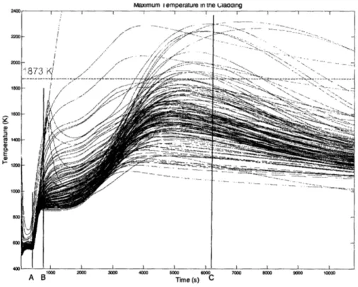
to the loss of mass flow rate through the core. Figure 8 shows 128 realizations for the

maximum cladding temperature. The horizontal dashed line corresponds to the

previously mentioned limit.

Maximum I emperature in tne UlaOing

-v

-00

1000 2000 3000 4000 5000 6000 7000 8000 9000 1000

A B Time (s) C

Figure 8 Realizations for Maximum Temperature in the Cladding

As expected, the maximum temperature in the cladding occurs after the shaft

stops (about 500 seconds after the LOCA

-

Point A in Figure 8). During this period, the

mass flow rate through the core reaches its minimum and the helium in the core,

becoming less dense because of the increasing temperature, tries to overcome the

4001 " , . I

--- --- --- ... _..

...

negative flow coming down from the leaking (both check valves are assumed to leak) of

the DHR loops. Eventually, one of the DHR check valves opens (Point B in Figure 8)

initiating the natural circulation through the core and the maximum temperature in the

cladding reduces its rate of change and ultimately comes down (Point C in Figure 8). It is

during this last period of time when realizations reach their maxima. There is one

realization for which the temperature never comes down and corresponds to the only case

in which the check valves never open because of the significant leakage in both of them.

There were 15 curves that exceeded the limit, so the overall probability for this failure

mode is 0.12. This probability is conditional on the LOCA.

The second failure mode corresponds to the structural failure of the operating

DHR Loop. As already stated, a limit of 850 C (1123 K) to the maximum temperature on

the hot legs (MTHL) was set as the failure criterion for this failure mode. Figure 9 shows

the 128 resulting realizations. Each realization is represented in the graph by two curves;

one for each DHR loop. The always decreasing curves correspond to the DHR loop with

the check valve closed. In the initial conditions of the simulation, the MTHL is set as if

there were no leakage in either loop. This is the worst possible initial condition because

the MTHL is smaller with leakage than without. This is due to the fact that the leaking

helium comes from the downcomer and passes through water cooled heat exchanger

where it cools down substantially. There were 26 curves that exceeded the limit, thus the

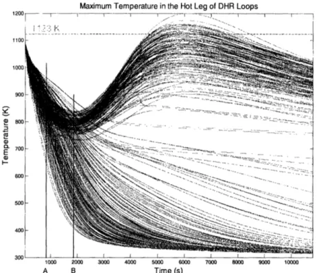
Maximum Temperature in the Hot Leg of DHR Loops 1200 -j T T FT F'F 1100 1000 900 ) 800 700 E I--600 500 400 300 i 1000 2000 3000 4000 5000 6000 7000 8000 9000 10000 A B Time (s)

Figure 9 Realizations for the Maximum Temperature in the Hot Leg of DHR Loops

As soon as the LOCA occurs, the MTHL starts decreasing in both loops because

of the injection of cold helium from the downcomer. When the check valve opens (Point

A in Figure 9), the behavior of the operating loop starts departing from the one that is still

leaking until it reaches a minimum at about 30 minutes (Point B in Figure 9). The reason

is that, once the valve opens, natural circulation starts building up and hotter helium

coming from the upper plenum heats up the pipes. From then on, the MTHL is well

correlated to the behavior of the maximum temperature in the cladding presented in

Figure 8.

The conditional failure probability is 0.305 when both failure modes are included.

Referring to the discussion in Section 3.5, we find that

F

=

39 over a total of 128

the total would be 41 instead of 39, if each realization led to a single failure. We

conclude that two realizations led to failures by both failure modes.

3.7 Insights

Interesting insights into the behavior of the system can be produced by developing

scatter plots of failures and successes for two parameters at a time (Ghosh and

Apostolakis, 2006). Figure 10 shows such a plot for the two leakages associated with

each Monte Carlo realization (one for each DHR loop) for the maximum temperature in

the cladding. On the horizontal axis we plot the maximum of the two leakages and on the

vertical axis the minimum. The plus signs indicate a realization and the square around a

plus sign indicates that this realization is, in fact, a failure of the cladding. Looking at the

lower left corner of the plot we observe that no failures exist below the dashed line.

Thus, we conclude that no cladding failure occurs when the maximum leakage in the

loops is less than about 0.8 kg/s and the minimum leakage is less than about 0.5 kg/s.

0.8 O.6 06 -00 0.4 0.2 co 0.5 CD 02 - 0.6 L0.4 0B 1 1.2 14 1.6 1 Max(Leakage 1, Leakage 2) [kg/s]

Figure 10 Leakage Threshold Effect (cladding failure)

I Ii _E3 19n 4 , 1 •-• + 1 -• . +. _if . . .. ,:•,_-.:*•. :,. _ , [ I II I l .8

The explanation for this behavior is the following: After the shaft stops, the

system attempts to open the check valves by overcoming the leakage. The valve with the

smallest leakage is the one that eventually opens. The higher the minimum leakage the

later the check valve opens. Such a delay means that more heat has been deposited in the

core with no extraction and therefore the temperature has increased.

Once the valve opens, natural circulation develops through the corresponding

DHR loop, but part of the fluid in the lower plenum is taken by the other DHR loop's

leakage and transferred directly to the upper plenum, thus bypassing the core. The higher

the maximum leakage, the smaller mass flow is available to the core for heat removal.

Failure is the combined effect of the two quantities and, as Figure 10 shows, only values

outside the lower triangle can lead to failure.

Threshold effects can be found for the structural failure mode as well. Figure 11

shows a similar plot for the effect of the HTCS and the maximum leakage of the valves.

The effect of the leakage is easily understood. The maximum leakage corresponds to the

loop whose check valve never opens and remains leaking after the other DHR loop starts

operating. That flow is inserting cold helium to the inlet of the operating DHR loop

through common upper plenum. Thus, if the maximum leakage is sufficiently high, it

cools down the upper plenum enough, preventing failure. As Figure 11 shows, there is

no structural damage when the HTCS factor is larger than 0.86 and the maximum leakage

is larger than 0.63 [kg/s]. Figure 11 also shows that there is no cladding damage when

the HTCS factor is smaller than 0.86 regardless of the value of the maximum leakage.

The explanation for this behavior is as follows: the lower the HTCS, the higher the

equalized. Higher pressure means higher helium density and, as explained in Section 2

(Equation 1), this corresponds to a smaller temperature difference across the core for the

same amount of extracted heat. Finally, the smaller temperature difference is translated

into a smaller core outlet temperature that reduces the probability of failure by MTHL.

+ -10 U1

~,

Figure 11 Maximum leakage and HTCS Threshold Effect (structural failure)

Insights into the behavior of the system can also be produced using the

Generalized Sensitivity Analysis (GSA) developed in (Hornberger and Spear, 1981) for

environmental systems. A GSA application to nuclear waste repositories is in (Ghosh

and Apostolakis, 2006). GSA partitions Monte Carlo realizations into two bins: one bin

contains all the realizations leading to failure and the other all the realizations not leading

to failure. We then look at the realizations in the failure bin and ask whether there are

iu 10 U) .E_ C/) 10'

any threshold effects, i.e., intervals of values of the input parameters that guarantee no

failure. The process will become clear using concrete examples.

Figure 12 shows the cumulative distribution function of the parameter on the

horizontal axis in the realizations that did not lead to cladding failure (continuous curve)

and the cumulative distribution function in the realizations that did lead to such failure

(staircase curve). Only the parameter HTCS shows a potential threshold effect in the

sense that failure would be very unlikely if the HTCS factor were less than about 0.48.

'--7 -,

I

.1

Figure 12 Search for threshold effects

0.9 0.8 0.7-0.6 0.5 0.4 0.3[ 0.2 0.1 10,2 10" 10' 10

-I

1..

Shaft Moment of Inertia (kg m2)

(Failure Mode 1, cladding failure)

Figure 13 shows the same type of graphs for the second failure mode (structural

failure). This time, the threshold effect on the HTCS is more pronounced. Failure only

4-/ / / '4 A f•t . . .. . ... . ... ... . • .. . .... . i t f lit

occurs if the value of the HTCS factor is greater than about 0.86, as found earlier (Fig.

10).

j

1

1[

Shaft Moment of Inertia (kg m2)

Figure 13 Search for threshold effects (Failure Mode 2, structural failure)

Both failure modes present threshold effects for the HTCS. Both failure modes

become very unlikely for small values of the HTCS factor because the pressure in the

containment can be maintained high for a longer period of time. This confirms an earlier

finding by Pagani et al., (2005) that containment pressure is a key parameter for the

success of natural circulation decay heat removal in gas cooled systems. Also, it is

important to note that containment leakage, which was not part of our studies, is another

important parameter that will negatively affect system performance in a similar manner

mode is not for the other. To prevent failure due to melting of the cladding, a small

maximum check valve leakage is desirable; but to prevent a structural collapse of the

8. RISK-BASED DESIGN CHANGES

The failure probability of 0.305 (conditional on the LOCA occurrence) is deemed

to be too high. Since a good amount of information about the system behavior under

different scenarios has been gathered, several actions can be taken. Since the dominant

failure mode is the structural collapse of a DHR loop (accounts for -2/3 of the total

failure probability), it is there where the first design change can be made. In the design

analyzed, the hot legs were simulated with adiabatic heat flux boundary conditions at the

outer periphery, which effectively corresponds to perfect insulation at this surface. The

design has been modified by placing the insulation on the inner surface of the pipe. This

way, the outer perimeter is cooled down by the cold leg flow (recall that cold leg is a

coaxial pipe surrounding the hot leg). However, heat losses through the insulation heat

up the cold leg flow reducing the buoyancy driving head and affecting the natural

circulation capability. Therefore, this solution also requires raising containment backup

pressure to achieve desired DHR performance.

Additional design changes are necessary to reduce the failure probability. The

backup pressure is a relatively strong factor on both failure modes since threshold effects

are visible for the HTCS factor in both failure modes, though they are of different

magnitudes. Therefore, an increase in containment backup pressure would substantially

reduce the failure probability. One possible way to achieve this is to insulate the steel

structures in the containment to minimize heat transfer to these structures and their effect

on pressure decrease. Another option is a gradual depressurization of the helium

inventory, into the containment. However, an increase in containment design pressure

with an associated cost increase would be required.

The primary concerns are the check valve leakage and core bypass phenomena

because of their strong effect on the performance of the passive system as a whole. The

use of more reliable check valves is of great significance to this design, but most

important is the observation that the redundancy of DHR loops can actually impair the

performance of the DHR system because the parallel loop can itself become a bypass.

Therefore, the smaller than 100% capacity DHR loops cannot be used and 100% capacity

loops are necessary. Nevertheless, any leak of check valves in parallel loops affects the

cooling capability of the core negatively. Thus, use of just one 100% DHR loop with a

reliable and leak-proof check valve would eliminate the possibility of core bypass and

provide the best performance, but such a solution is unrealistic since no perfect valves

exist. Consequently, the use of a combination of active and passive systems for DHR or

of a fully active DHR with reliable backup power need to be considered and, in fact, may

9. CONCLUSIONS

From an overall perspective, the first important conclusion is that the passive

system design process has to incorporate a reliability assessment. The complexity of the

system and the overall impact of the simultaneous variation of several input parameters

makes it impossible for the designer to foresee every possible situation.

The reliability evaluation process provides useful information to the designer. At

an early stage, the analysis of the system components gives a starting point as to where

the hazards may be; the most insightful view, however, comes later with the second and

third screenings during the mechanistic analysis and after the uncertainty propagation.

During the mechanistic analysis, improvements to the design can be made in view of the

evidence given by nominal simulations and sensitivity analyses. The probabilistic

analysis produces insights that the nominal analysis does not produce. In Figures 8 and

9, the curves that exceed the damage limits are the results of specific combinations of the

values of the input parameters. The curves corresponding to the nominal values are

below the limits and do not reveal the possibility of failure. In addition, the sensitivity

analysis allows the discovery of threshold effects in the input parameters and the

potential combined effect of two of them in two-dimensional scatter plots.

We point out that the probabilistic analysis presented here is different from the

usual use of PSA in design. In the latter case, several design configurations are analyzed

and compared using a metric such as the core damage frequency (Mizuno et al, 2005;

Delaney et al, 2005). These studies are performed at the system level and usually lead to

mechanistic model for a safety function and investigates the impact of uncertainties in the

input parameters on the probability of function failure. This process reveals the

significance of certain possible values of the input parameters and leads to design

changes that affect these values. It is closer to the analysis presented by Ghosh and

Apostolakis (2006) for nuclear waste repositories.

The sensitivity analyses identify potential threshold effects in the input parameters

and lead to a better understanding of the dynamics of the system. This understanding is

very helpful in efforts to improve the design in an effective way. Since one design

change may affect the behavior of several failure modes differently, it is crucial to

understand their interactions for the success of the design improvement. Finally, the

single failure probabilities and the safety function failure probability provide a

10.REFERENCES

ANS, 1979. American National Standard

for Decay Heat Power in Light Water

Reactors, ANSI/ANS-5.1-1979, American Nuclear Society, La Grange

Park, Illinois.

Apostolakis, G.E., 1994. "A commentary on model uncertainty," in: Proceedings of

Workshop on Model Uncertainty: Its Characterization and Quantification,

Annapolis, MD, October 20-22, 1993. A. Mosleh, N. Siu, C. Smidts, and

C. Lui, Eds., Report NUREG/CP-0138, US Nuclear Regulatory

Commission, Washington, DC.

Burgazzi, L., 2003. "Reliability evaluation of passive systems through functional

reliability assessment." Nuclear Technology, 144:145-151.

Burgazzi, L., 2004. "Evaluation of uncertainties related to passive systems

performance." Nuclear Engineering and Design, 230:93-106.

Delaney, M.J., Apostolakis, G.E., and Driscoll, M.J., 2005. "Risk-informed design

guidance for future reactor systems." Nuclear Engineering and Design,

235:1537-1556.

Ghosh, S. T., Apostolakis, G.E., 2006. "Extracting risk insights from performance

assessments for high-level radioactive waste repositories." Nuclear

Technology, 153:70-88.

Hejzlar, P., Kim, S.J., and Williams, W.C., 2005. Transient A THENA/RELAP5-3D

Calculations

for a 600MWth Plate-Type Helium GFR, MIT Report

MIT-GFR-026, Massachusetts Institute of Technology, Cambridge, MA.

Helton, J.C., Davis, J.F., 2003. "Latin hypercube sampling and the propagation of

uncertainty in analyses of complex systems." Reliability Engineering &

System Safety, 81:23-69.

Hornberger, G.M., Spear, R.C., 1981. "An approach to the preliminary analysis of

environmental systems." Journal ofEnvironmental Management, 12:7-18.

IAEA, 1991. Safety Related Terms for Advanced Nuclear Power Plants,

TEC-DOC-626. International Atomic Energy Agency, Vienna, Austria.

INEEL, 2001. RELAP5-3D© code manual volume I: code structure, system models,

and solution methods. INEEL-EXT-98-00834, Idaho National

Engineering and Environmental Laboratory, Idaho Falls, Idaho.

Jafari, J., D'Auria, F., Kazeminejad, H., Davilu, H., 2003. "Reliability evaluation of

a natural circulation system." Nuclear Engineering and Design,

224:79-104.

Lee, J.I., and Hejzlar, P., 2007. "Experimental and Computational Analysis of Gas

Natural Circulation Loop", Proceedings of the International Congress on

Advances in Nuclear Power Plants ICAPP '07, Paper 7381, Nice, France,

May 13-18.

Marques, M, Pignatel, J.F., Saignes, P., D'Auria, F., Burgazzi, L., Miller, C.,

Bolado-Lavin, R., Kirchsteiger, C., La Lumia, V., and Ivanov, I., 2005.

"Methodology for the reliability evaluation of a passive system and its

integration into a probabilistic safety assessment." Nuclear Engineering

and Design, 235:2612-2631.

Mizuno, Y., Ninokata, H., and Finnicum, D.J., 2005. "Risk-informed design of IRIS

using a level-1 probabilistic risk assessment from its conceptual design

phase." Reliability Engineering and System Safety, 87:201-209.

Pagani, L.P., Apostolakis, G.E., and Hejzlar, P., 2005. "The impact of uncertainties

on the performance of passive systems," Nuclear Technology,

149:129-140.

Zio, E, Cantarella, M, Cammi, A., 2003. "The analytic hierarchy process as a

systematic approach to the identification of important parameters for the

reliability assessment of passive systems." Nuclear Engineering and

Design, 226:311-336.

11. APPENDICES

11.2.

APPENDIX B: RELAP5-3D NOMINAL INPUT DECK

*crdno end time min dt max dt control minor ed major ed restart

201 10800.0 1.0-10 0.0025 23 400 800000 400000 * * *

*---* Reactor Coolant System

*---*

301 p 750010000 * Water Loops Data

302 tempf 750010000 * 303 p 751010000 * 304 tempf 751010000 * 305 p 750200000 * 306 tempf 750200000 * 307 p 751200000 * 308 tempf 751200000 * 309 mflowj 750010000 * 310 mflowj 751010000 * 311 cntrlvar 126 * q from 710 312 cntrlvar 127 * q from 711 313 cntrlvar 128 * q from 750 314 cntrlvar 129 * q from 751 315 p 710010000 * 316 tempf 710010000 * 317 p 711010000 * 318 tempf 711010000 * 319 p 710050000 * 320 tempf 710050000 * 321 p 711050000 * 322 tempf 711050000 * * *

DHR Loops Data 323 324 325 326 327 328 329 330 331 332 333 334 335 336 337 338 339 340 341 342 343 344 345 346 347 348 * * 349 350 351 352 353 354 355 356 357 358 359 360 361 362 363 364 365 367 368 369 370 371 372 373 374 375 376 377 378 p P p p P p g tempg tempg tempg tempg mflowj mflowj cntrlvar cntrlvar P p tempg p tempg p tempg p tempg p tempg p tempg httemp httemp p p p p tempg tempg tempg tempg p p p p tempg tempg tempg tempg mflowj mflowj mflowj mflowj mf 1 owj p tempg p tempg cntrlvar cntrlvar cntrl1var cntrlvar 650010000 651010000 650050000 651050000 650010000 651010000 650050000 651050000 665000000 674000000 120 125 610050000 610050000 611050000 611050000 666010000 666010000 676010000 676010000 666050000 666050000 676050000 676050000 610100101 611100101 250010000 251010000 250080000 251080000 250010000 251010000 250080000 251080000 670010000 670080000 800010000 800080000 670010000 670080000 800010000 800080000 250010000 251010000 670010000 800010000 300040000 300050000 300050000 100010000 100010000 111 102 123 110 * * * * * * * * * * * Reactor and Downcomer Data

Q extracted from rector Estimated Q extracted Q generated by the reactor Max temp fuel 251 httemp