Environmental Satisfaction in Open-Plan Environments: 3. Further Scale Validation

(1)

Publisher’s version / Version de l'éditeur:

Vous avez des questions? Nous pouvons vous aider. Pour communiquer directement avec un auteur, consultez la première page de la revue dans laquelle son article a été publié afin de trouver ses coordonnées. Si vous n’arrivez pas à les repérer, communiquez avec nous à PublicationsArchive-ArchivesPublications@nrc-cnrc.gc.ca.

Questions? Contact the NRC Publications Archive team at

PublicationsArchive-ArchivesPublications@nrc-cnrc.gc.ca. If you wish to email the authors directly, please see the first page of the publication for their contact information.

https://publications-cnrc.canada.ca/fra/droits

L’accès à ce site Web et l’utilisation de son contenu sont assujettis aux conditions présentées dans le site LISEZ CES CONDITIONS ATTENTIVEMENT AVANT D’UTILISER CE SITE WEB.

Research Report (National Research Council of Canada. Institute for Research in

Construction), 2003-10-16

READ THESE TERMS AND CONDITIONS CAREFULLY BEFORE USING THIS WEBSITE. https://nrc-publications.canada.ca/eng/copyright

NRC Publications Archive Record / Notice des Archives des publications du CNRC :

https://nrc-publications.canada.ca/eng/view/object/?id=b78e9748-f264-4b66-bc99-7a8e2648e515 https://publications-cnrc.canada.ca/fra/voir/objet/?id=b78e9748-f264-4b66-bc99-7a8e2648e515

NRC Publications Archive

Archives des publications du CNRC

For the publisher’s version, please access the DOI link below./ Pour consulter la version de l’éditeur, utilisez le lien DOI ci-dessous.

https://doi.org/10.4224/20378165

Access and use of this website and the material on it are subject to the Terms and Conditions set forth at

Environmental Satisfaction in Open-Plan Environments: 3. Further

Scale Validation

(2)

Environmental Satisfaction in Open-Plan

Environments: 3. Further Scale Validation

Kate E. Charles, Jennifer A. Veitch, Kelly M. J.

Farley, and Guy R. Newsham

IRC Research Report RR-152

Oct. 16, 2003

(3)

Environmental Satisfaction in Open-Plan Environments: 3. Further Scale Validation

Environmental Satisfaction in Open-Plan Environments:

3. Further Scale Validation

Kate E. Charles, Jennifer A. Veitch, Kelly M. J. Farley, and Guy R. Newsham IRC, National Research Council of Canada

Executive Summary

The COPE field study was designed to determine the effects of open-plan office design on the indoor environment and occupant satisfaction with that environment. Extensive local physical

measurements, combined with simultaneous questionnaire data, were collected from 779 workstations in nine government and private sector office buildings, in large Canadian and US cities. This report describes a confirmation of the factor structure for the questionnaire component, established in an earlier COPE report (Veitch, Farley, & Newsham, 2002).

The questionnaire measured occupants’ satisfaction with 18 environmental features, their overall environmental satisfaction, and job satisfaction. We hypothesised that the 18 environmental features ratings could be meaningfully reduced to a smaller number of underlying latent variables. Our earlier analyses examined this hypothesis using exploratory and confirmatory factor analysis, and determined a three-factor structure reflecting satisfaction with privacy/acoustics, satisfaction with lighting and satisfaction with ventilation. In the current analysis, confirmatory factor analysis supported this three-factor structure, and the new data achieved a comparable fit to this model. Our use of data from different geographical locations and organisational sectors supports the generalisability of this framework. Our findings are also broadly consistent with other researchers, who typically find three to five factors, including those for lighting, ventilation and noise/privacy.

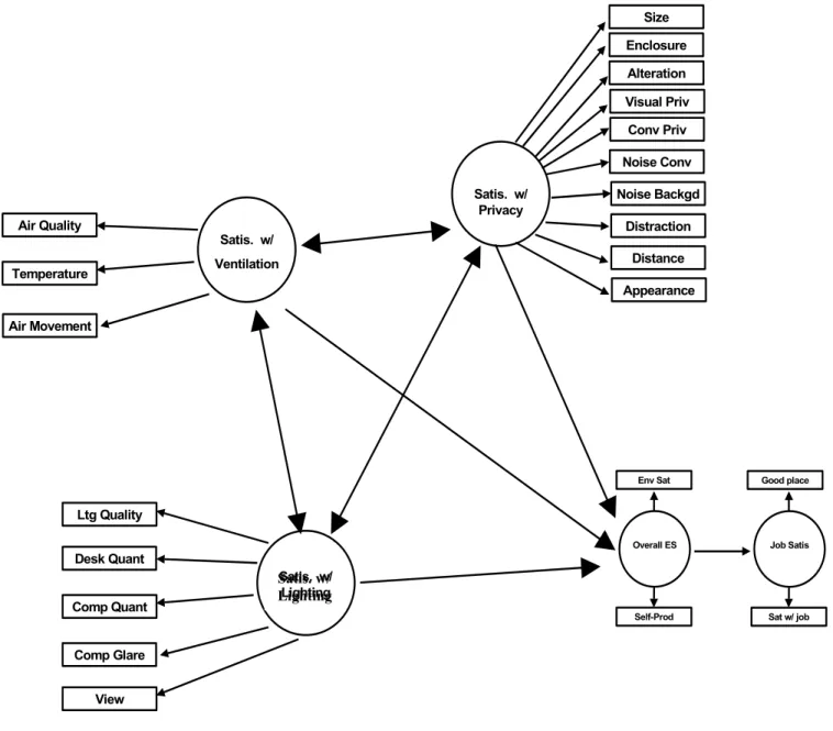
In our earlier analyses, we also examined relationships between the environmental features ratings, overall environmental satisfaction, and job satisfaction. We hypothesised that the three factors (described above) would be related to overall environmental satisfaction, which in turn would be related to job satisfaction (see Fig. A). The model tested achieved acceptable fit to the data and the hypothesised relationships were statistically significant. In the current analysis, this structural equation model was retested using the full COPE dataset. The data achieved a comparable fit to the model, suggesting it to be a valid conceptualisation of the relationships between the variables.

Our results are consistent with those of other researchers, suggesting that occupants who are more satisfied with their physical environment also report greater job satisfaction. This relationship is

particularly important, given the role of job satisfaction in predicting wider organisational outcomes, such as commitment, intent to turnover, customer satisfaction, and absenteeism.

(4)

Figure A. Relationships between field study questionnaire items Satis. w/ Ventilation Air Quality Temperature Air Movement Desk Quant Comp Quant Comp Glare View Ltg Quality Satis. w/ Privacy Alteration Enclosure Distance Appearance Size Conv Priv Noise Backgd Distraction Visual Priv Noise Conv Overall ES Env Sat Self-Prod Job Satis Good place Sat w/ job Satis. w/ Lighting Satis. w/ Lighting

(5)

1.0 Introduction... 5 2.0 Method ... 6 2.1 Sites ... 6 2.1.1 Building 1 details... 7 2.1.2 Building 2 details... 7 2.1.3 Building 3 details... 7 2.1.4 Building 4 details... 9 2.1.5 Building 5 details... 9 2.1.6 Building 6 details... 9 2.1.7 Building 7 details... 10 2.1.8 Building 8 details... 10 2.1.9 Building 9 details... 10 2.2 Participants ... 10 2.3 Questionnaire Measures ... 12 3.0 Results... 12

3.1 Descriptive Statistics and Data Screening ... 12

3.2 Subsamples... 13

3.2.1 CFA Sample... 13

3.2.2 SEM Sample. ... 15

3.3 Confirmatory Factor Analysis ... 18

3.4 Relations to Overall Environmental Satisfaction and Job Satisfaction ... 20

4.0 Discussion ... 21

5.0 References... 22

Acknowledgements... 23

Appendix A: Complete CFA Models... 24

Appendix B: Complete SEM Models ... 26

Tables and Figures Table 1. Summary of site characteristics………... ..8

Table 2. Demographic characteristics of participants………... 11

Table 3. Descriptive statistics: CFA sample………. 13

Table 4. Intercorrelations between environmental features ratings for CFA sample……….... 14

Table 5. Descriptive statistics: SEM sample………. 16

Table 6. Intercorrelations between all items for SEM group……… 17

Table 7. CFA results: Goodness of fit indices……….. 19

Table 8. SEM results: Goodness of fit indices……….. 20

Figure 1. Relationships between field study questionnaire items………. ..6

Figure 2. CFA model………. 19

Figure 3. SEM model……… 21

Environmental Satisfaction in Open-Plan Environments: 3. Further Scale Validation

(6)

Kate E. Charles, Jennifer A. Veitch, Kelly M. J. Farley & Guy R. Newsham

Institute for Research in Construction National Research Council of Canada

October 16, 2003

1.0 Introduction

The Cost-effective Open-Plan Environments (COPE) field study was designed to determine the effects of open-plan office design on the indoor environment and on occupant satisfaction with that environment. It combines extensive local physical measurements with simultaneous questionnaire data collection. Data for this study were collected from 779 individual workstations in nine government and private sector office buildings, located in large Canadian and US cities.

This report concerns only the questionnaire component of the COPE field study. The questionnaire measured occupants’ satisfaction with 18 environmental features, their overall

environmental satisfaction, and job satisfaction. We hypothesised that the 18 environmental features ratings could be meaningfully reduced to a smaller number of underlying latent variables. This factor reduction would provide a smaller, more manageable and interpretable set of subscales that could be used in further analyses. We also hypothesised that these subscales would be related to overall environmental satisfaction and job satisfaction.

Following data collection from three buildings in 2000 (n=419), the factor structure of

questionnaire responses was examined (see Veitch, Farley, & Newsham, 2002). Using exploratory factor analysis, we determined that the 18 environmental features ratings could be reduced to three subscales, reflecting satisfaction with privacy/acoustics, lighting, and ventilation, respectively. Confirmatory factor analysis supported this model, and we found acceptable fit between the model and the data from these buildings.

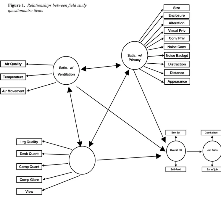
We then used structural equation modeling to test the relationships between the three environmental subscales, overall environmental satisfaction, and job satisfaction. The model tested consisted of the three subscales (intercorrelated) which jointly affected overall environmental satisfaction, which in turn affected job satisfaction (see Figure 1). This model achieved acceptable fit to the data from these buildings, and all relationships were found to be statistically significant.

In 2002, the dataset was expanded by including data from six further buildings (n=360; full dataset, n=779). We tested the models described above against this expanded dataset, to determine their fit in relation to the newly acquired data. Confirmation of the models’ fit, and statistical significance of the relationships within them, provide us with greater confidence that the models developed are valid and can be meaningfully used in further analyses of the COPE field study data. In this report, we describe the results of these analyses, and compare them to those found using the original dataset.

(7)

Environmental Satisfaction in Open-Plan Environments: 3. Further Scale Validation Satis. w/ Ventilation Air Quality Temperature Air Movement Satis. w/ Lighting Satis. w/ Lighting Desk Quant Comp Quant Comp Glare View Ltg Quality Satis. w/ Privacy Alteration Enclosure Distance Appearance Size Conv Priv Noise Backgd Distraction Visual Priv Noise Conv Overall ES Env Sat Self-Prod Job Satis Good place Sat w/ job Figure 1. Relationships between field study

questionnaire items

2.0 Method

The data collection method has been described in detail in a previous COPE report (Veitch, et al, 2002). Therefore, the scope of this section is restricted to information directly relevant to our current analyses.

2.1 Sites

Data were collected in nine office buildings, located in large Canadian and US cities. The first three buildings were occupied by federal government organisations in large Canadian cities, and were visited in 2000. The dataset was expanded in 2002, by including data from four private-sector office buildings (one organisation), and two provincial government office buildings (one organisation). Three of the buildings were in large Canadian cities, and the remaining buildings were located in a two US cities. All buildings, and the specific locations within them, were selected because they contained open-plan offices occupied by white-collar workers, and because their management was willing to host the

(8)

visit. During the 2002 data collection, we also intentionally chose buildings that contained smaller workstations and lower partitions, to increase the presence of these workstation characteristics in the overall dataset. A summary of the building characteristics at each site is shown in Table 1.

Parts of four floors in the eastern half of this building were visited. Office accommodation at this location was primarily open-plan, with some enclosed offices on the perimeter and at the centre of the floor plan. In the majority of cases, open-plan workstations were formed using free-standing fabric partitions, and free-standing furniture elements. Lighting was provided, almost universally, by surface mounted prismatic luminaires housing a single 4ft fluorescent lamp. These luminaires were located at the centre of 5ft x 5ft ceiling coffer elements. Sound masking was not in use at this location. The HVAC system comprised a ducted-air variable air volume (VAV) cooling system, and a perimeter hot-water heating system, both controlled by zone thermostats. Perimeter zones stretched between structural columns along the perimeter (33ft) to a depth of about 10ft; interior zones were up to 30ft x 30ft in size. The building operators controlled zone thermostats. Thermostats were generally fixed at 22oC, although certain thermostats had been adjusted to

accommodate local preferences. The VAV system utilised two compartment fans in each tower of each floor. Each fan served approximately half the floor plate, and was capable of supplying up to 25,500 cfm, with the outside air fraction fixed at 10%. Manual controls ensured that the flow rate to the interior zones never fell below 50% of maximum, and that the flow rate to the perimeter zones never fell below 20% of maximum. These fans were switched off between 6pm – 6am each night; only the fans serving the building lobby and retail floors operated for 24 hours/day.

2.1.1 Building 1 details.

Areas of three floors were visited. Office accommodation at this location was primarily open-plan, with some enclosed offices on the perimeter and at the centre of the floor plan. In the majority of cases, open-plan workstations were formed using systems furniture elements. Lighting was provided, almost universally, by recessed paracube parabolic luminaires housing a single 4ft fluorescent lamp. Orange-painted hollow ceiling beam-like elements formed a 5ft x 5ft ceiling grid, and each of these 5ft x 5ft areas contained one (usually) luminaire at the centre (usually). Sound masking was not in use at this location. The ceiling beams also contained slot air diffusers. The HVAC system comprised a ducted-air VAV cooling system, and a perimeter convection heating system. Zones served by individual VAV boxes were approximately 1500 ft2, though some smaller perimeter zones had been created where solar gain was problematic. The building operators controlled zone thermostats. The target thermostat setting was 22oC, though many thermostats had been adjusted to accommodate local preferences. The building had two main fresh air fans with in-line heating and cooling coils; there was also a cooling coil in the main return air duct. The VAV system utilised two compartment fans on each floor. Each fan served approximately half the floor plate, with the outside air fraction fixed at 15%. Controls ensured that the flow rate to the interior zones never fell below 10% of maximum. These fans were switched off between 6pm – 2am each night.

Sections of four floors were visited, two in spring and two in winter. Office accommodation at this location was primarily open-plan, with some enclosed offices at the centre of the floor plan. In the majority of cases, open-plan workstations were formed using systems furniture elements. Lighting was provided, almost universally, by ceiling-recessed prismatic luminaires housing a single 4’ fluorescent lamp, though there were “paracube” parabolic luminaires in a few locations. These luminaires were located in a regular grid on 5ft x 5ft centres. Sound masking was used on all floors at this location. The HVAC system comprised a ducted-air VAV cooling system, and a perimeter hot- and chilled-water system. The perimeter system was locally controlled by occupants. The VAV system was controlled by zone thermostats in the interior; interior zones were up to 15ft x 20ft in size. Zones were originally aligned with office locations, but

rearrangement of office furniture over the years means that 2.1.3 Building 3 details.

(9)

Table 1. Summary of site characteristics. Building Year

Built

City Sector Visited # Floors Floor plate (sf)

Lighting HVAC Windows Sound

1 1977 Ottawa public spring 2000 11 (4 visited) 39,000 (x 2 towers) 4' coffered prismatic fluorescent

ducted air VAV cooling / perimeter hot-water heating

non-operable no sound masking 2 1975 Toronto public summer

2000

12 (3 visited)

40,000 4' recessed parabolic cube

ducted air VAV cooling / perimeter convention heating

non-operable no sound masking 3 1975 Ottawa public spring

2000 & winter 2000 22 (4 visited) 18,000 4' recessed prismatic (some parabolic)

ducted air VAV cooling / perimeter hot and chilled water heating & cooling

non-operable sound masking in use 4 1976 Ottawa private winter

2002

15 (1 visited)

16,000 2’ x 4’ prismatic ducted air VAV cooling / perimeter hot-water heating

non-operable no sound masking 5 1994 San Rafael private spring

2002 3 (3 visited)

40,000 2’ x 4’ recessed parabolic

ducted air VAV cooling / hot-water reheat

non-operable sound masking in use 6 1984 San Rafael private spring

2002 5 (1 visited)

35,000 2’ x 4’ recessed parabolic

ducted air VAV cooling / perimeter hot-water heating non-operable no sound masking 7 1916 (renovated 2000) San Francisco private spring 2002 8 (1 visited)

41,000 8’ direct/ indirect ducted air VAV operable windows

sound masking in specific locations 8 1954 Montreal public spring

2002 4 (2 visited) 6,700 50% indirect / 50% 2’x 4’ parabolic

ducted air VAV / perimeter heating non-operable no sound masking 9 1989/90 Quebec City public spring 2002 3 (3 visited)

15,300 1’ x 4’ parabolic Fan-coil with occupant-controlled ceiling vents, perimeter electric heating

non-operable no sound masking

(10)

this is no longer the case. The building operators controlled interior zone thermostats. Thermostats were initially set at 20-22 oC, although certain thermostats had been adjusted to accommodate local

preferences. The VAV system utilised a total of seven fans, four dedicated to the interior and three to the perimeter. Perimeter fans served South, North-east and North-west zones. The outside air fraction varied with external climate, but never fell below 15 %. These fans were switched off between 6pm – 6am each night.

Measurements were taken in various areas of one floor of this building. The office accommodation was primarily open-plan, with some enclosed. In the majority of cases, open-plan workstations were formed using systems furniture elements. Lighting was provided, almost universally, by ceiling-recessed 2ft x 4ft, prismatic lens

luminaires housing two 4ft fluorescent lamps, these luminaires were located in a regular grid on 6ft x 10ft centres. There were supplemental undershelf task lighting in most workstations. The HVAC system comprised a VAV system, with hot water perimeter heating. The VAV system was controlled by

pnuematic control thermostats in each zone; the zone sizes are 1200 ft2 on the interior, and every 10 linear ft on the perimeter. Building occupants chose the local thermostat settings. Total air flow to the floor was 40,000 cfm; the outside air fraction varied between 20% and 100%. The system fans were switched off between 9pm – 6 am.

Data were collected from all three floors of this building. The office accommodation was primarily open-plan, with some enclosed offices on the 1st floor. In the majority of cases, open-plan workstations were formed using systems furniture elements. Lighting was provided, almost universally, by ceiling-recessed 2ft x 4ft, 18-cell, deep-cell parabolic luminaires housing three 4’ fluorescent lamps, these luminaires were located in a regular grid on 8ft x 12ft centres. There were some supplemental 2ft x 2ft luminaires in some locations, as well as

undershelf task lighting. Sound masking was in use in this building. The HVAC system comprised a VAV system, with hot water reheat. The VAV system was controlled by pnuematic control thermostats in each zone; the zone sizes vary based on design, exposure, and usage. The facilities managers set the thermostats at approximately 72 F (22.2 oC). The outside air fraction varied with external climate, but never fell below 20%; free cooling was utilized and outside air fraction could rise to 100% to maximize this. The system fans were switched off between 6pm – 4.30 am each workweek night, and were off all weekend. The organisation we visited at this building had a policy allowing occupants to bring pets, principally dogs, to work. This policy was indicated to be a privilege, and there were requirements for behavioural standards to be met. This organisation also supported work-from-home arrangements.

One floor was visited in this building. The office accommodation was a mixture of enclosed offices and open-plan, though

measurements were conducted in open-plan offices only. In the majority of cases, open-plan workstations were formed using systems furniture elements. Lighting was provided, almost universally, by ceiling-recessed 2ft x 4ft, 18-cell, deep-cell parabolic luminaires housing three 4ft fluorescent lamps, these luminaires were located in a regular grid on 8ft x 12ft or 8ft x 10ft centres. There was some use of supplemental undershelf task lighting. There was no sound masking system in use in this building. The HVAC system comprised a VAV system, with hot water perimeter coils. The VAV system was

controlled by pnuematic control thermostats in each zone; there were typically 3-4 offices per zone. The building managers and tenants interact in setting the thermostats at approximately 70-72 F (21.1-22.2 oC) in summer and 74F (23.3 oC) in winter. Air flow rates were around 1.5-2 cfm/ft2. The outside air fraction was 15-20%. The system fans were switched off between 6pm – 6 am (except Monday when they were started earlier at 4.30 am). The organisation visited at this building also had pets-at-work and work-from-home policies.

(11)

Measurements were taken on one floor of this building. The office accommodation was entirely open-plan, with a few enclosed

conference rooms. Open-plan workstations were formed using systems furniture elements. Lighting was provided, almost universally, by 8ft direct/indirect luminaires housing a single fluorescent lamp, these luminaires were suspended 18 inch. from the ceiling in regular rows. The HVAC system comprised a VAV system only. The VAV system was controlled by zone thermostats in each zone; zones varied in size. The tenants set the thermostats locally at typically 71-73 F (21.7-22.8 oC). Outside air supply was 20 cfm/person, based on 133 ft2/person. The outside air fraction was at least 20% of total air flow. The system fans were switched off between 6pm – 7 am each weekday night. Windows at the building perimeter were openable. The organisation visited at this building also supported work-from-home arrangements.

Two floors were visited in this building. The office accommodation was mostly open-plan, formed using systems furniture elements. Fifty percent of the lighting in the areas visited was provided by indirect lighting luminaires (2 lamps per 4ft length), suspended 16 inch. from the ceiling. The remaining lighting was provided by 2ft x 4ft parabolic “paracube” luminaires housing 2 lamps. These luminaires were located in a regular grid on 8ft x 6ft centres. Workstations also had adjustable “angle-arm” task lights. Sound masking was not in use in this building. The HVAC system comprised a VAV system, capable of supplying 18,265 l/s airflow, and was supplemented with perimeter heating. The VAV system was controlled by direct digital control for each 100 m2 zone. The fraction of outside air varied with external climate, but was never allowed to fall below 17%. Outside airflow was typically around 0.9-1.2 cfm/ft2. Thermostats were located at the centre of groups of four workstations, and were usually adjusted by occupants. The system was switched off between 6pm and 2.30am each workweek night, and were off all weekend.

All three floors of this building were visited. The office

accommodation was mainly open-plan, formed using systems furniture elements. Lighting was provided by 1ft x 4ft deep-cell parabolic luminaires, housing 2 lamps, with one luminaire assigned for every 50 ft2 of floor area. Sound masking was not in use in this building. The HVAC system used fan coil units to provide local cooling needs. Constant airflow volume was provided meeting a minimum outdoor air supply rate of 10 ls-1/person. Occupants had control of a ceiling diffuser dedicated to their workstation, and could change the direction of airflow, or close the diffuser entirely. Thermostats, to which occupants had access, controlled zones of 400-500 ft2. Perimeter heating was provided by electric baseboard heaters. The HVAC system was turned off at night and on weekends.

2.1.9 Building 9 details

2.2 Participants

Participants were the occupants of floors visited by the research team. All occupants present on the visit day were eligible to participate, and approximately 90% of those invited agreed to take part. Table 2 shows the demographic characteristics for the full sample, the original (3-building) sample, the new (6-building) sample, and each individual building.

(12)

Table 2. Demographic characteristics of participants.

Site N % English % female /% male Mean age (SD)

Full sample 779 79.5 47.6 / 51.5 36.2 (10.6) Original 3 buildings 419 87.6 48.7 / 50.4 38.6 (10.8) New 6 buildings 360 70.0 46.4 / 52.8 33.5 (9.5) Building 1 132 85.6 47.7 / 51.5 38.2 (12.7) Building 2 160 98.8 48.8 / 50.6 37.8 (9.4) Building 3 127 75.6 49.6 / 48.8 39.5 (10.1) Building 4 52 94.2 23.1 / 75.0 32.1 (8.0) Building 5 85 97.6 67.1 / 31.8 33.1 (9.6) Building 6 48 100.0 62.5 / 37.5 29.8 (9.4) Building 7 72 100.0 31.9 / 68.1 30.7 (7.3) Building 8 47 0.0 53.2 / 44.7 38.8 (9.9) Building 9 56 0.0 35.7 / 64.3 37.3 (10.1)

Job Category (%) Administration Technical Professional Management

Full sample 27.1 24.9 38.4 8.6 Original 3 buildings 36.0 14.8 41.3 6.7 New 6 buildings 16.7 36.7 35.0 10.8 Building 1 18.9 11.4 68.2 0.0 Building 2 47.5 11.3 32.5 8.1 Building 3 39.4 22.8 24.4 11.8 Building 4 1.9 57.7 30.8 7.7 Building 5 20.0 20.0 41.2 17.6 Building 6 33.3 14.6 35.4 16.7 Building 7 6.9 52.8 25.0 15.3 Building 8 31.9 34.0 29.8 2.1 Building 9 10.7 42.9 46.4 0.0

Education (%) High School Community College University Courses Undergraduate Degree Graduate Degree Full sample 11.6 15.1 14.6 34.0 22.7 Original 3 buildings 16.0 17.7 14.6 26.0 23.2 New 6 buildings 6.4 12.2 14.7 43.3 22.2 Building 1 9.1 8.3 13.6 30.3 37.1 Building 2 13.1 21.3 16.9 26.3 20.0 Building 3 26.8 22.8 12.6 21.3 12.6 Building 4 0.0 5.8 13.5 36.5 42.3 Building 5 4.7 3.5 12.9 58.8 17.6 Building 6 6.3 8.3 18.8 41.7 25.0 Building 7 2.8 5.6 19.4 48.6 23.6 Building 8 12.8 27.7 14.9 25.5 17.0 Building 9 14.3 30.4 8.9 35.7 10.7

(13)

2.3 Questionnaire Measures

Workstation occupants were asked to indicate their workplace satisfaction and demographic information by answering a questionnaire presented on a palmtop computer. Occupants were instructed to base their responses on the physical conditions that existed at the time they were asked to participate in the study. In addition to the five demographic questions described above, occupants responded to 22 satisfaction items.

Environmental Features Ratings (EFR): The first 18 questions asked occupants to rate their satisfaction with various aspects of the indoor environment (e.g., “the amount of lighting on the desktop”, “the overall air quality in your work area”, “the level of privacy for conversations in your office.”). Occupants responded on a 7-point scale which ranged from “very unsatisfactory” to “very satisfactory”. These items were based primarily on work by Stokols and Scharf (1990).

Overall Environmental Satisfaction (OES): Two items were used to rate occupants’ satisfaction with the physical environment as a whole. The first asked occupants to assess, on the same 7-point scale used above, how satisfied they felt overall about their environment (Stokols & Scharf, 1990). The second item asked participants to rate how the environment influenced their productivity at the time of the survey, relative to general prevailing conditions, using a scale which ranged from “30% less productive” to “30% more productive” than usual (Wilson & Hedge, 1987).

Job Satisfaction (JS): The final two items were used to assess job satisfaction. These items were drawn with minor modifications from a recent survey for the Canadian federal public service (Ross, 1999). Occupants responded, on a 7-point scale ranging from “very strongly disagree” to “very strongly agree”, to these items.

The full wording for each item can be found in Section 3.2.2, Table 5.

3.0 Results

The purpose of the current analyses was to examine the factor structure of the questionnaire data and compare it to that found in previous analyses. To validate the factor structure of the 18

environmental features ratings, we used confirmatory factor analysis, using the new data collected in 2002 (n=360). To test the relationships between the environmental features ratings, overall environmental satisfaction, and job satisfaction, we subjected the full dataset (n=779) to structural equation modelling analysis.

3.1 Descriptive Statistics and Data Screening

The questionnaire data were transformed from their original format (Microsoft Excel) into a data file that could be read by EQS for Windows 6.1 (Bentler & Wu, 2003). A careful review of the

transformed data confirmed the accuracy of data input. Data preparation and screening was conducted using the procedures recommended by Kline (1997). The dataset was examined for missing data. Variable mean imputation was used where missing data was infrequent and randomly distributed. Cases with missing data on multiple items were excluded from the analysis. Univariate normality was assessed by examining the kurtosis and skewness values of the individual items. According to Kline, skewness values greater than an absolute value of 3 and kurtosis values greater than an absolute value of 8 indicate univariate normality problems. Univariate outliers were identified by examining frequency distributions of standardised scores. Scores greater than 3 standard deviations from the mean were excluded from analysis. Multivariate normality was assessed by examining randomly selected bivariate scatterplots for linearity and homoscedasticity, and by assessing the normality of randomly selected joint distributions of combinations of the variables. Multivariate outliers were detected by examining the values of the Mahalanobis distance statistic. Cases for which the Mahalanobis distance statistic was greater than the critical value at p<.001 were excluded from the analysis. Correlation matrices were examined to check for multicollinearity and singularity. Circumstances in which items are highly correlated (r>.80) indicate potential multicollinearity problems, because understanding their separate relations to other variables

(14)

becomes difficult. Items that are only weakly correlated with other variables (r<.30) suggest that the variable is singular, and does not have meaningful relations to other items.

3.2 Subsamples

Two subsamples were created for the analyses. The first sample was used to conduct the

confirmatory factor analysis (CFA), and consisted of all cases from the new data collection (buildings 4 to 9; n=360). The second sample was used to test the structural equation model (SEM) and consisted of the full dataset (buildings 1 to 9; n=779).

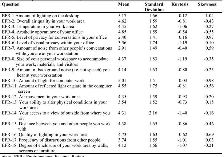
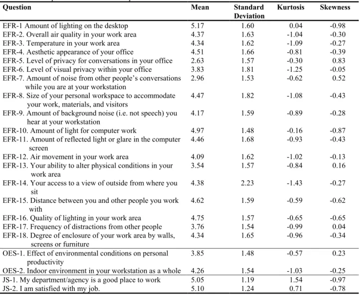
The data for the CFA analysis was screened in accordance with the above procedure. The mean, standard deviation, kurtosis and skewness for the first 18 satisfaction items are presented in Table 3 (other variables are not included because they were not used in the CFA). Two cases had missing data on all questionnaire items, and so were excluded from the analysis. The proportion of missing data for other cases was very low (2.5%) and appeared to be random. Therefore, the variable mean was substituted for each missing observation (Kline, 1997).

3.2.1 CFA Sample.

For this dataset, the maximum skewness value was –1.04 and the maximum kurtosis value was -1.40. Therefore, the items can all be considered to be normally distributed. There were no univariate outliers. Examination of randomly selected bivariate and combined variable scatterplots suggested that multivariate normality could be assumed. Five cases were identified as multivariate outliers, using Mahalanobis distance statistic at p<.001, and were removed from the analysis. Following data screening, the remaining sample for the CFA analysis was n=353.

Table 3. Descriptive statistics: CFA sample

Question Mean Standard

Deviation

Kurtosis Skewness EFR-1 Amount of lighting on the desktop 5.17 1.66 0.12 -1.04 EFR-2. Overall air quality in your work area 4.62 1.59 -0.81 -0.43 EFR-3. Temperature in your work area 4.45 1.62 -1.06 -0.27 EFR-4. Aesthetic appearance of your office 4.85 1.59 -0.54 -0.55 EFR-5. Level of privacy for conversations in your office 2.40 1.41 0.16 0.97 EFR-6. Level of visual privacy within your office 3.56 1.74 -1.19 0.10 EFR-7. Amount of noise from other people’s conversations

while you are at your workstation

2.91 1.49 -0.40 0.59

EFR-8. Size of your personal workspace to accommodate your work, materials, and visitors

4.37 1.83 -1.19 -0.35

EFR-9. Amount of background noise (i.e. not speech) you hear at your workstation

4.14 1.63 -0.80 -0.25

EFR-10. Amount of light for computer work 5.01 1.51 0.03 -0.98 EFR-11. Amount of reflected light or glare in the computer

screen

4.55 1.75 -0.81 -0.56

EFR-12. Air movement in your work area 4.35 1.59 -0.93 -0.20 EFR-13. Your ability to alter physical conditions in your

work area

3.54 1.52 -0.73 0.15

EFR-14. Your access to a view of outside from where you sit

4.31 2.16 -1.40 -0.16

EFR-15. Distance between you and other people you work with

4.38 1.65 -0.86 -0.46

EFR-16. Quality of lighting in your work area 4.73 1.63 -0.62 -0.69 EFR-17. Frequency of distractions from other people 3.74 1.55 -1.01 0.03 EFR-18. Degree of enclosure of your work area by walls,

screens or furniture

4.12 1.66 -1.07 -0.21

(15)

Table 4. Intercorrelations between environmental features ratings for CFA sample.

EFR-1 EFR-2 EFR-3 EFR-4 EFR-5 EFR-6 EFR-7 EFR-8 EFR-9 EFR-10 EFR-11 EFR-12 EFR-13 EFR-14 EFR-15 EFR-16 EFR-17 EFR-18 EFR-1 1.00 EFR-2 0.35 1.00 EFR-3 0.17 0.54 1.00 EFR-4 0.35 0.32 0.15 1.00 EFR-5 0.10 0.22 0.21 0.27 1.00 EFR-6 0.13 0.10 0.05 0.22 0.58 1.00 EFR-7 0.13 0.18 0.16 0.15 0.65 0.52 1.00 EFR-8 0.12 0.13 0.10 0.30 0.32 0.37 0.32 1.00 EFR-9 0.17 0.30 0.25 0.32 0.28 0.32 0.41 0.28 1.00 EFR-10 0.69 0.37 0.19 0.40 0.16 0.18 0.18 0.24 0.24 1.00 EFR-11 0.35 0.25 0.18 0.29 0.18 0.21 0.16 0.25 0.21 0.58 1.00 EFR-12 0.21 0.67 0.55 0.28 0.13 0.10 0.18 0.06 0.33 0.27 0.24 1.00 EFR-13 0.19 0.30 0.24 0.40 0.42 0.34 0.37 0.41 0.40 0.30 0.29 0.30 1.00 EFR-14 0.20 0.15 -0.02 0.15 0.04 0.07 0.12 0.17 0.10 0.21 -0.05 0.04 0.07 1.00 EFR-15 0.18 0.20 0.13 0.24 0.43 0.46 0.49 0.42 0.37 0.26 0.17 0.10 0.38 0.18 1.00 EFR-16 0.66 0.43 0.19 0.45 0.17 0.18 0.21 0.26 0.31 0.76 0.45 0.37 0.31 0.26 0.24 1.00 EFR-17 0.11 0.21 0.22 0.20 0.49 0.51 0.67 0.37 0.48 0.21 0.21 0.20 0.36 0.01 0.57 0.22 1.00 EFR-18 0.20 0.19 0.08 0.34 0.45 0.61 0.47 0.43 0.37 0.27 0.22 0.18 0.42 0.08 0.57 0.33 0.54 1.00

(16)

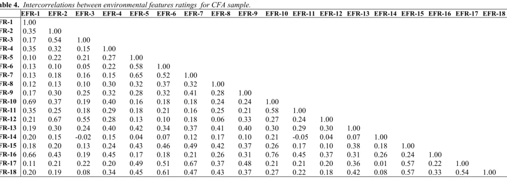
To test for multicollinearity and singularity, a correlation matrix for the 18 satisfaction items was constructed (Table 4). No correlations were greater than 0.80, suggesting an absence of multicollinearity. One item (“access to a view from where you sit”) was not correlated above 0.30 with any of the other 17 items, indicating potential singularity problems. A number of other items also had only a limited number of correlations above 0.30. However, given that these variables had a strong theoretical reason for being included in the questionnaire, and were also included in the original CFA analysis (Veitch et al, 2002), we decided to keep these items in the dataset.

The data for the SEM analysis was screened in accordance with the above procedure. The mean, standard deviation, kurtosis and skewness for all items is shown in Table 5. Three cases had missing data on all questionnaire items, and were excluded from the analysis. There were 59 cases that had missing data for one or more items. In 20 of these cases, missing data was minimal and appeared random, so variable mean substitution was used. In the

remaining 39 cases, there was missing data for multiple items, or for items that load on the same subscale. As mean substitution was not an appropriate strategy in these circumstances, these cases were excluded from the analysis.

3.2.2 SEM sample.

As is shown in Table 5, the maximum skewness value for this dataset was -0.98, and the maximum kurtosis value was 1.54. Therefore, all items can be considered to be normally distributed. There were 18 cases with standardised scores more than 3 standard deviations from the mean. As these univariate outliers would unduly bias the analysis, they were removed from the dataset. Examination of randomly selected bivariate and combined variable scatterplots suggested that multivariate normality could be assumed. Five cases were identified as multivariate outliers, using Mahalanobis distance statistic at p<.001, and were removed from the analysis. Following data screening, the remaining sample for the SEM analysis was n=714.

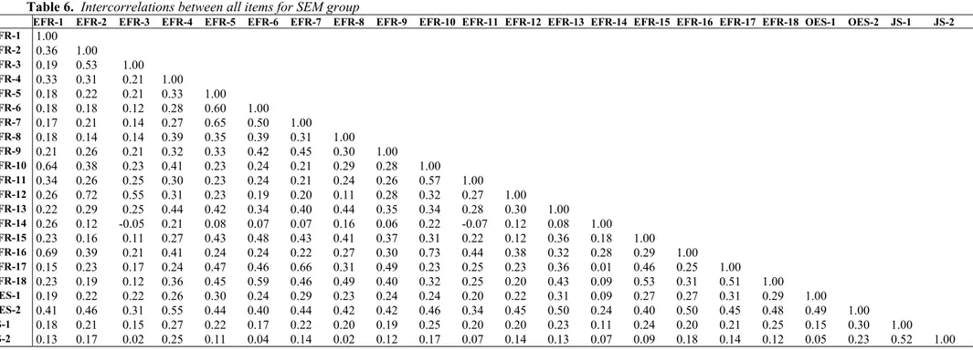
The dataset was examined for multicollinearity and singularity, using a correlation matrix for all 22 items (Table 6). The largest correlation was 0.73, therefore multicollinearity was unlikely to be problematic. The item “access to a view from where you sit” was again only weakly correlated (r<0.30) with other items, indicating potential singularity problems. A number of other items also had only limited correlations over 0.30. However, given that there is strong theoretical reason for including these items in the questionnaire, and in the original SEM analysis (Veitch et al, 2002), these items were retained.

(17)

Table 5. Descriptive statistics: SEM sample

Question Mean Standard

Deviation

Kurtosis Skewness EFR-1 Amount of lighting on the desktop 5.17 1.60 0.04 -0.98 EFR-2. Overall air quality in your work area 4.37 1.63 -1.04 -0.30 EFR-3. Temperature in your work area 4.34 1.62 -1.09 -0.27 EFR-4. Aesthetic appearance of your office 4.51 1.66 -0.81 -0.39 EFR-5. Level of privacy for conversations in your office 2.63 1.57 -0.30 0.83 EFR-6. Level of visual privacy within your office 3.83 1.81 -1.25 -0.05 EFR-7. Amount of noise from other people’s conversations

while you are at your workstation

2.96 1.53 -0.62 0.52

EFR-8. Size of your personal workspace to accommodate your work, materials, and visitors

4.47 1.82 -1.08 -0.43

EFR-9. Amount of background noise (i.e. not speech) you hear at your workstation

4.17 1.59 -0.89 -0.28

EFR-10. Amount of light for computer work 4.97 1.48 -0.16 -0.87 EFR-11. Amount of reflected light or glare in the computer

screen

4.46 1.68 -0.93 -0.43

EFR-12. Air movement in your work area 4.09 1.62 -1.02 -0.13 EFR-13. Your ability to alter physical conditions in your

work area

3.54 1.57 -0.84 0.16

EFR-14. Your access to a view of outside from where you sit

4.38 2.23 -1.43 -0.27

EFR-15. Distance between you and other people you work with

4.62 1.59 -0.59 -0.62

EFR-16. Quality of lighting in your work area 4.75 1.57 -0.65 -0.65 EFR-17. Frequency of distractions from other people 3.76 1.54 -0.99 0.04 EFR-18. Degree of enclosure of your work area by walls,

screens or furniture

4.34 1.65 -0.96 -0.34

OES-1. Effect of environmental conditions on personal productivity

3.85 1.48 -0.57 0.23

OES-2. Indoor environment in your workstation as a whole 4.26 1.54 -1.03 -0.25 JS-1. My department/agency is a good place to work 5.05 1.19 1.54 -0.97 JS-2. I am satisfied with my job. 5.10 1.24 0.71 -0.78 Note. EFR: Environmental Features Rating. OES: Overall Environmental Satisfaction. JS: Job Satisfaction.

(18)

Table 6. Intercorrelations between all items for SEM group

EFR-1 EFR-2 EFR-3 EFR-4 EFR-5 EFR-6 EFR-7 EFR-8 EFR-9 EFR-10 EFR-11 EFR-12 EFR-13 EFR-14 EFR-15 EFR-16 EFR-17 EFR-18 OES-1 OES-2 JS-1 JS-2 EFR-1 1.00 EFR-2 0.36 1.00 EFR-3 0.19 0.53 1.00 EFR-4 0.33 0.31 0.21 1.00 EFR-5 0.18 0.22 0.21 0.33 1.00 EFR-6 0.18 0.18 0.12 0.28 0.60 1.00 EFR-7 0.17 0.21 0.14 0.27 0.65 0.50 1.00 EFR-8 0.18 0.14 0.14 0.39 0.35 0.39 0.31 001. EFR-9 0.21 0.26 0.21 0.32 0.33 0.42 0.45 0.30 1.00 EFR-10 0.64 0.38 0.23 0.41 0.23 0.24 0.21 0.29 0.28 1.00 EFR-11 0.34 0.26 0.25 0.30 0.23 0.24 0.21 0.24 0.26 0.57 1.00 EFR-12 0.26 0.72 0.55 0.31 0.23 0.19 0.20 0.11 0.28 0.32 0.27 1.00 EFR-13 0.22 0.29 0.25 0.44 0.42 0.34 0.40 0.44 0.35 0.34 0.28 0.30 1.00 EFR-14 0.26 0.12 -0.05 0.21 0.08 0.07 0.07 0.16 0.06 0.22 -0.07 0.12 0.08 1.00 EFR-15 0.23 0.16 0.11 0.27 0.43 0.48 0.43 0.41 0.37 0.31 0.22 0.12 0.36 0.18 1.00 EFR-16 0.69 0.39 0.21 0.41 0.24 0.24 0.22 0.27 0.30 0.73 0.44 0.38 0.32 0.28 0.29 1.00 EFR-17 0.15 0.23 0.17 0.24 0.47 0.46 0.66 0.31 0.49 0.23 0.25 0.23 0.36 0.01 0.46 0.25 1.00 EFR-18 0.23 0.19 0.12 0.36 0.45 0.59 0.46 0.49 0.40 0.32 0.25 0.20 0.43 0.09 0.53 0.31 0.51 1.00 OES-1 0.19 0.22 0.22 0.26 0.30 0.24 0.29 0.23 0.24 0.24 0.20 0.22 0.31 0.09 0.27 0.27 0.31 0.29 1.00 OES-2 0.41 0.46 0.31 0.55 0.44 0.40 0.44 0.42 0.42 0.46 0.34 0.45 0.50 0.24 0.40 0.50 0.45 0.48 0.49 1.00 JS-1 0.18 0.21 0.15 0.27 0.22 0.17 0.22 0.20 0.19 0.25 0.20 0.20 0.23 0.11 0.24 0.20 0.21 0.25 0.15 0.30 1.00 JS-2 0.13 0.17 0.02 0.25 0.11 0.04 0.14 0.02 0.12 0.17 0.07 0.14 0.13 0.07 0.09 0.18 0.14 0.12 0.05 0.23 0.52 1.00

(19)

3.3 Confirmatory Factor Analysis

Confirmatory factor analysis is a form of structural equation modelling, in which the investigator specifies a model that is expected to describe the observed data. The fit of the model to the data is evaluated against several criteria, the pattern of which leads to a judgement as to whether the fit is acceptably good or not (Kline, 1997).

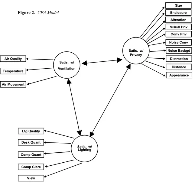
In the original analyses (Veitch et al, 2002), the factor structure of the 18 environmental features ratings was examined, to determine the model to be tested. The original 3-building dataset (n=419) was randomly split into two subsamples for this investigation. Using one subsample, a three-factor solution was determined, using exploratory factor analysis. The three factors underlying the 18 environmental features ratings were satisfaction with privacy/acoustics, lighting, and ventilation, respectively. The second subsample was then used to test this 3-factor model (see Figure 2), using confirmatory factor analysis, and an acceptable fit to the data was found.

In the current analysis, we used confirmatory factor analysis to test the model again, this time using data from the new buildings (buildings 4-9). The fit of the model to this data was then compared against that from the previous analysis.

The model submitted for analysis consisted of maximum likelihood estimations of the 18 target loadings, three factor variances, correlations between all factors and error variances for each of the 18 items (see Figure 2). Model fit was assessed using multiple statistical and fit indices including Chi-square, Goodness of Fit Index (GFI), Adjusted Goodness of Fit Index (AGFI), Bentler-Bonett Normed Fit Index (NFI), Bentler-Bonett Non-normed Fit Index (NNFI) and the Standardised Root Mean Square Residual (RMSR.) Detailed descriptions of these and other indices can be found in several sources (e.g., Byrne, 1994; Kline, 1997; Tabachnick & Fidell, 2001). Briefly, a low and non-significant value of the chi-square statistic indicates a good fit to the data. However, chi-square can not be interpreted in a standardised way (it has no theoretical upper bound) and is very sensitive to sample size. To deal with the sensitivity to sample size problem, the chi-square statistic can be divided by the degrees of freedom to get a better estimate. Kline (1997) suggested that a chi-square/df ratio of less than 3 is acceptable. Generally, statisticians recommend a multiple set of fit indices should be examined (Byrne, 1994; Kline, 1997; Tabachnick & Fidell, 2001). The GFI and AGFI values range from 0 (poor fit) to 1 (perfect fit). The GFI is analogous to a squared multiple correlation indicating the proportion of covariances explained by the model-implied covariances, whereas the AGFI is like a shrinkage-corrected squared multiple correlation in that it includes an adjustment for model complexity (Kline, 1997). The NFI indicates the proportion in the improvement of the overall fit of the model to a null model (one in which the observed variables are assumed to be uncorrelated), compared to the NNFI which includes a correction for model complexity similar to the AGFI. NFI and NNFI values range from 0-1. Tabachnick and Fidell (2001) suggested that GFI, AGFI, NFI and NNFI values of 0.9 or greater indicate the model is a good fit to the data. In contrast, the RMSR is a standardised summary of the covariance residuals that indicates better fit with lower (closer to zero) values.

Table 7 summarises the results of the original and new CFAs, including optimal values for the various fit indices. In comparison to the original CFA, the new CFA shows poorer fit in relation to the

Χ2_{/df fit index (4.00 as compared to 2.75). However, this statistic is sensitive to sample size, and so this}

result is, to some extent, an effect of increased sample size in the current analysis. In addition, the results show small improvements in fit for most of the remaining fit indices (GFI, AGFI, NFI, and NNFI). In both the original and the new CFAs, all parameter estimates are statistically significant (see Appendix A). Overall, the new data fit the model shown in Figure 2 as well as the original data, suggesting that the model developed from the original analysis remains applicable.

(20)

Satis. w/ Ventilation Air Quality Temperature Air Movement Satis. w/ Lighting Desk Quant Comp Quant Comp Glare View Ltg Quality Satis. w/ Privacy Alteration Enclosure Distance Appearance Size Conv Priv Noise Backgd Distraction Visual Priv Noise Conv

Figure 2. CFA Model

Table 7. CFA results: Goodness of fit indices

N Χ2 Χ2/df GFI AGFI NFI NNFI RMSR

Optimal fit < 3 > .90 >.90 >.90 >.90 <.10

Original CFA 205 363.40 2.75 .83 .77 .78 .82 .07

New CFA 353 527.63 4.00 .85 .81 .82 .83 .08

Note. Both CFAs tested against model shown in Figure 2. Full results with parameter estimates are shown in Appendix A. Optimal values and their sources are described in the text.

To determine whether a different model would fit the data more appropriately, the Legrange Multiplier (LM) test and the Wald W statistic were examined to determine possible misfits. The LM test provides an estimate of how much the overall chi-square statistic would decrease if a particular parameter were added. Conversely, the Wald W test estimates the amount the overall chi-square would increase if a particular free parameter were fixed, that is, dropped from the model. In both the original and the new CFAs, the Wald W test indicated that the model would not be improved by dropping any parameters. In the original analysis, the LM test indicated the model could be improved by adding a parameter from the variable “the aesthetic appearance of your office” to the factor “satisfaction with lighting”. Satisfaction

(21)

with the appearance of one’s office or workspace might reasonably be related to the quality of lighting available. In the original analysis, a new model with this added parameter was tested, but was not found to significantly improve model fit. Any such improvements were out-weighted by the additional

complexity of a cross-loading item (a variable contributing to more than one factor). The cross-loading item would have complicated the interpretation of further analyses. The LM test for the new CFA also suggested the addition of the same parameter. However, given the conclusions reached during the original CFA, there was no justification to modify the model. The three-factor model provides an acceptable fit to both the original and the new data.

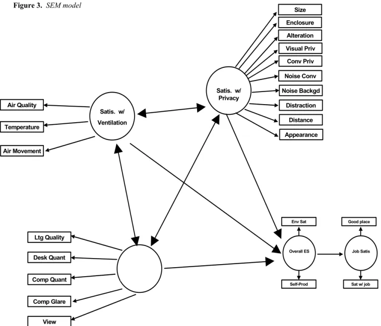
3.4 Relations to Overall Environmental Satisfaction and Job Satisfaction

In the original analyses (Veitch et al, 2002), structural equation modelling was used to examine relationships between the environmental features ratings, overall environmental satisfaction and job satisfaction. The model developed and tested consisted of the three, intercorrelated, factors (identical to the CFA model, Figure 2), plus unidirectional paths from each factor to overall environmental

satisfaction, and a unidirectional path from overall environmental satisfaction to job satisfaction. The composite overall environmental satisfaction factor consisted of two items (“indoor environment in your workstation as a whole” and “effect of environmental conditions on personal productivity”), and the composite job satisfaction factor consisted of two items (“I am satisfied with my job” and “my

department/agency is a good place to work”). This model is shown in Figure 3, and an acceptable fit was found between the model and the original 3-building data.

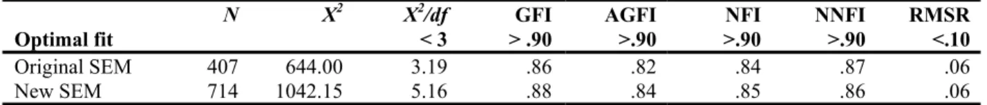
In the current analysis, this structural equation model was tested against the full dataset (buildings 1-9). The fit of the model was then compared to that found in the original analyses. Table 8 summarises these results.

Table 8. SEM results: Goodness of fit indices

N Χ2 Χ2/df GFI AGFI NFI NNFI RMSR

Optimal fit < 3 > .90 >.90 >.90 >.90 <.10

Original SEM 407 644.00 3.19 .86 .82 .84 .87 .06

New SEM 714 1042.15 5.16 .88 .84 .85 .86 .06

Note. Both SEMs tested against model shown in Figure 3. Full results with parameter estimates are shown in Appendix B. Optimal values and their sources are described in the text.

As Table 8 indicates, the Χ2/df fit index suggests a poorer model fit for the new SEM, as

compared to the original analysis (1042.15 as compared to 644). However, as mentioned above, this fit statistic is sensitive to sample size. As the new SEM analysis is based on almost twice as many cases as the original analysis, it is not surprising that this index shows a poorer fit. However, the remaining fit statistics show identical or slightly improved fit for the new SEM, as compared to the original (GFI, AGFI, NFI, NNFI, RMSR). In both the original and the new SEMs, all parameter estimates were statistically significant (see Appendix B). Taken as a whole, the results suggest that the model shown in Figure 3 is a valid conceptualisation of the relationships between the variables, and that this model acceptably fits the full COPE field study dataset.

In the new SEM, LM and Wald W tests were examined, to determine possible improvements to the model. The Wald W statistic indicated that the model would not be improved by dropping any parameters. The LM test indicated that the model could be improved by adding a parameter from the variable “the aesthetic appearance of your office” to the factor “overall environmental satisfaction”. However, the addition of this parameter would add a cross-loading item to the model, thereby increasing complexity of interpretation. This added complexity was unlikely to be justified by a significant increase in model fit, and so we decided not to include this extra parameter in the model. The model described in Figure 3 adequately fits the full dataset, and is clear and easily interpretable.

(22)

Satis. w/ Ventilation Air Quality Temperature Air Movement Satis. w/ Lighting Satis. w/ Lighting Desk Quant Comp Quant Comp Glare View Ltg Quality Satis. w/ Privacy Alteration Enclosure Distance Appearance Size Conv Priv Noise Backgd Distraction Visual Priv Noise Conv Overall ES Env Sat Self-Prod Job Satis Good place Sat w/ job Figure 3. SEM model

4.0 Discussion

The COPE field study was designed to determine the effects of open-plan office design on the indoor environment and occupant satisfaction with that environment. Extensive local physical

measurements, combined with simultaneous questionnaire data, were collected from 779 workstations in nine government and private sector office buildings, in large Canadian and US cities. This report describes a confirmation of the factor structure for the questionnaire component, established in an earlier COPE report (Veitch et al, 2002).

We hypothesised that the 18 environmental features ratings that we measured could be meaningfully reduced to a smaller number of underlying latent variables. In the original analysis, we examined this hypothesis using exploratory and confirmatory factor analysis, and determined a three-factor structure reflecting satisfaction with privacy/acoustics, satisfaction with lighting and satisfaction with ventilation. In the new analysis, further confirmatory factor analysis supported this three-factor structure, and the new data achieved a comparable fit to this model. Our findings are broadly consistent

(23)

with other researchers, who typically find three to five factors, including those for lighting, ventilation and noise/privacy (e.g. González, Fernández, & Cameselle, 1997; Veitch & Newsham, 1998).

It is interesting to note that the new data, against which this model was tested, included both public and private sector organisations. It is often argued that these organisational types are

fundamentally different, and so cannot be viewed in the same way. However, our results indicate that the tested model fits both public and private sector data comparably. It appears that public and private sector employees respond to their physical environments in similar ways, and that the model we developed is generalisable to both sectors.

The original analyses (Veitch et al, 2002) also examined relationships between the environmental features ratings, overall environmental satisfaction, and job satisfaction. We hypothesised that the three factors (described above) would be related to overall environmental satisfaction, which in turn would be related to job satisfaction. The structural equation model tested (see Figure 3) achieved acceptable fit to the data and the hypothesised relationships were statistically significant. In the new analysis, this

structural equation model was retested using the full COPE dataset. The data achieved a comparable fit to the model, suggesting it to be a valid conceptualisation of the relationships between the variables. The results also indicated that the inclusion of data from the private sector did not reduce the model fit, suggesting that this model is applicable to both public and private sector organisations.

Our results are consistent with those of other researchers, suggesting that occupants who are more satisfied with their physical environment also report greater job satisfaction (e.g. Dillon & Visher, 1987; Donald & Siu, 2001; Wells, 2000). This relationship is important, given the role of job satisfaction in predicting wider organisational outcomes. Several researchers have demonstrated that job satisfaction is related to organisational outcomes such as commitment, intent to turnover, customer satisfaction, and absenteeism (e.g. Carlopio, 1996; Hardy, Woods, & Wall, 2003; Hellman, 1997; Koys, 2001, Shaw, 1999). In a recent study, Harter, Schmidt, and Hayes (2002) conducted a meta-analysis on 198,514 employees from 7,939 business-units in 36 companies, to examine the relationships between employee satisfaction and organisational outcomes. Their findings indicated that the average job satisfaction for each business-unit was consistently related to business-unit customer satisfaction, turnover, accidents, productivity and profitability. Our results, therefore, suggest that satisfaction with the physical environment may indirectly contribute to wider organisational outcomes; a hypothesis that warrants further attention in future work.

5.0 References

Byrne, B. M. (1994). Structural equation modeling with EQS and EQS/Windows: Basic concepts,

applications, and programming. Thousand Oaks, CA: Sage Publications.

Carlopio, J. R. (1996). Construct validity of a physical work environment satisfaction questionnaire.

Journal of Occupational Health Psychology, 1, 330-344.

Dillon, R., & Vischer, J. C. (1987). Derivation of the Tenant Questionnaire Survey assessment method:

Office building occupant survey data analysis. Ottawa, ON: Architectural and Engineering

Services. Public Works Canada.

Donald, I., & Siu, O. (2001). Moderating the stress impact of environmental conditions: The effect of organizational commitment in Hong Kong and China. Journal of Environmental Psychology,

21(4), 353-368.

González, M. S. R., Fernández, C. A., & Cameselle, J. M. S. (1997). Empirical validation of a model of user satisfaction with buildings and their environments as workplaces. Journal of Environmental

Psychology, 17, 69-74.

Hardy, G. E., Woods, D., & Wall, T. D. (2003). The impact of psychological distress on absence from work. Journal of Applied Psychology, 88(2), 306-314.

Harter, J. K., Schmidt, F. L., & Hayes, T. L. (2002). Business-unit-level relationship between employee satisfaction, employee engagement, and business outcomes: A meta-analysis. Journal of Applied

Psychology, 87(2), 268-279.

(24)

Hellman, C. M. (1997). Job satisfaction and intent to leave. Journal of Social Psychology, 137, 677-689.

Kline, R. B. (1997). Principles and practice of structural equation modeling. New York: Guilford Press.

Koys, D. J. (2001). The effects of employee satisfaction, organizational citizenship behavior, and turnover on organizational effectiveness: A unit-level, longitudinal study.

Ross, E. (1999). Public service employee opinion survey. Ottawa, ON: Special Survey Division. Statistics Canada.

Shaw, J. D. (1999). Job satisfaction and turnover intentions: The moderating role of positive affect.

Journal of Social Psychology, 139(2), 242-244.

Stokols, D., & Scharf, F. (1990). Developing standardised tools for assessing employees' ratings of facility performance. In G. Davis, & F. T. Ventre (Eds.), Performance of Buildings and

Serviceability of Facilities (pp. 55-68). Philadelphia, PA: American Society for Testing and

Materials.

Tabachnick, B., & Fidell, L. (2001). Using multivariate statistics (5th ed.). Boston: Allyn and Bacon. Veitch, J. A., Farley, K. M. J., Newsham, G. R. (2002). Environmental satisfaction in open-plan

environments: 1. Scale validation and methods (IRC-IR-844). Ottawa, ON: National Research

Council of Canada, Institute for Research in Construction.

Veitch, J. A., & Newsham, G. R. (1998). Lighting quality and energy-efficiency effects on task performance, mood, health, satisfaction and comfort. Journal of the Illuminating Engineering

Society, 27(1), 107-129.

Wells, M. M. (2000). Office clutter or meaningful personal displays: The role of office personalization in employee and organizational well-being. Journal of Environmental Psychology, 20, 239-255. Wilson, S., & Hedge, A. (1987). The office environment survey. London, UK: Building Use Studies

Ltd.

Acknowledgements

This investigation forms part of the Field Study sub-task for the NRC/IRC project Cost-effective Open-Plan Environments (COPE) (NRCC Project # B3205), supported by Public Works and Government Services Canada, Natural Resources Canada, the Building Technology Transfer Forum, Ontario Realty Corp, British Columbia Buildings Corp, USG Corp, and Steelcase, Inc. COPE is a multi-disciplinary project directed towards the development of a decision tool for the design, furnishing, and operation of open-plan offices that are satisfactory to occupants, energy-efficient, and cost-effective. Information about the project is available at http://irc.nrc-cnrc.gc.ca/ie/cope

The authors are grateful to the following individuals: Chantal Arsenault, Emily Nichols, Marcel Brouzes, Roger Marchand, John Bradley, Scott Norcross, Raymond Demers, Brian Fitzpatrick, Tim Estabrooks, Nathalie Brunette, Ralston Jaekel, Judy Jennings, and Ryan Eccles (data collection); Louise Legault (research design advice); Gordon Bazana, Cara Duval, and Clinton Marquardt (data

(25)