Publisher’s version / Version de l'éditeur:
The Astrophysical Journal Supplement Series, 238, 1, 2018-09-26
READ THESE TERMS AND CONDITIONS CAREFULLY BEFORE USING THIS WEBSITE. https://nrc-publications.canada.ca/eng/copyright
Vous avez des questions? Nous pouvons vous aider. Pour communiquer directement avec un auteur, consultez la première page de la revue dans laquelle son article a été publié afin de trouver ses coordonnées. Si vous n’arrivez pas à les repérer, communiquez avec nous à [email protected].
Questions? Contact the NRC Publications Archive team at
[email protected]. If you wish to email the authors directly, please see the first page of the publication for their contact information.
NRC Publications Archive
Archives des publications du CNRC
This publication could be one of several versions: author’s original, accepted manuscript or the publisher’s version. / La version de cette publication peut être l’une des suivantes : la version prépublication de l’auteur, la version acceptée du manuscrit ou la version de l’éditeur.
For the publisher’s version, please access the DOI link below./ Pour consulter la version de l’éditeur, utilisez le lien DOI ci-dessous.
https://doi.org/10.3847/1538-4365/aada7f
Access and use of this website and the material on it are subject to the Terms and Conditions set forth at
The JCMT Gould Belt Survey: SCUBA-2 data reduction methods and
Gaussian source recovery analysis
Kirk, Helen; Hatchell, Jennifer; Johnstone, Doug; Berry, David; Jenness, Tim;
Buckle, Jane; Mairs, Steve; Rosolowsky, Erik; Francesco, James Di;
Sadavoy, Sarah; J. Currie, Malcolm; Broekhoven-Fiene, Hannah; Mottram,
Joseph C.; Pattle, Kate; Matthews, Brenda; Knee, Lewis B. G.;
Moriarty-Schieven, Gerald; Duarte-Cabral, Ana; Tisi, Sam; Ward-Thompson, Derek
https://publications-cnrc.canada.ca/fra/droits
L’accès à ce site Web et l’utilisation de son contenu sont assujettis aux conditions présentées dans le site LISEZ CES CONDITIONS ATTENTIVEMENT AVANT D’UTILISER CE SITE WEB.
NRC Publications Record / Notice d'Archives des publications de CNRC:
https://nrc-publications.canada.ca/eng/view/object/?id=85390c08-0a86-4014-84e9-1b960d0b32c2 https://publications-cnrc.canada.ca/fra/voir/objet/?id=85390c08-0a86-4014-84e9-1b960d0b32c2
The JCMT Gould Belt Survey: SCUBA-2 Data Reduction Methods and Gaussian Source
Recovery Analysis
Helen Kirk1,2 , Jennifer Hatchell3 , Doug Johnstone1,2 , David Berry4, Tim Jenness5,6 , Jane Buckle7,8, Steve Mairs4 , Erik Rosolowsky9 , James Di Francesco1,2 , Sarah Sadavoy10 , Malcolm J. Currie5,11 , Hannah Broekhoven-Fiene2,
Joseph C. Mottram12,13, Kate Pattle14,15 , Brenda Matthews1,2 , Lewis B. G. Knee1 , Gerald Moriarty-Schieven1 , Ana Duarte-Cabral16, Sam Tisi17, and Derek Ward-Thompson14
1
NRC Herzberg Astronomy and Astrophysics Research Centre, 5071 West Saanich Road, Victoria, BC, V9E 2E7, Canada
2Department of Physics and Astronomy, University of Victoria, 3800 Finnerty Road, Victoria, BC, V8P 5C2, Canada 3
Physics and Astronomy, University of Exeter, Stocker Road, Exeter EX4 4QL, UK
4
East Asian Observatory, 660 N. A‘ohōkū Place, University Park, Hilo, HI 96720, USA
5
Joint Astronomy Centre, 660 N. A‘ohōkū Place, University Park, Hilo, HI 96720, USA6 LSST Project Office, 933 N. Cherry Avenue, Tucson, AZ 85719, USA
7
Astrophysics Group, Cavendish Laboratory, J J Thomson Avenue, Cambridge, CB3 0HE, UK
8
Kavli Institute for Cosmology, Institute of Astronomy, University of Cambridge, Madingley Road, Cambridge, CB3 0HA, UK
9
Department of Physics, University of Alberta, Edmonton, AB T6G 2E1, Canada
10
Harvard-Smithsonian Center for Astrophysics, 60 Garden Street, Cambridge, MA 02138, USA
11RAL Space, Rutherford Appleton Laboratory, Harwell Oxford, Didcot, Oxfordshire, OX11 0QX, UK 12
Leiden Observatory, Leiden University, P.O. Box 9513, 2300 RA Leiden, The Netherlands
13Max-Planck Institute for Astronomy, Königstuhl 17, D-69117 Heidelberg, Germany 14
Jeremiah Horrocks Institute, University of Central Lancashire, Preston, Lancashire, PR1 2HE, UK
15
Institute of Astronomy and Department of Physics, National Tsing Hua University, Hsinchu 30013, Taiwan
16
School of Physics and Astronomy, Cardiff University, The Parade, Cardiff, CF24 3AA, UK
17
Department of Physics and Astronomy, University of Waterloo, Waterloo, ON, N2L 3G1, Canada Received 2018 July 3; revised 2018 August 10; accepted 2018 August 13; published 2018 September 26
Abstract
The James Clerk Maxwell Telescope (JCMT) Gould Belt Survey (GBS) was one of the first legacy surveys with the JCMT in Hawaii, mapping 47 deg2of nearby (<500 pc) molecular clouds in dust continuum emission at 850 and 450 μm, as well as a more limited area in lines of various CO isotopologues. While molecular clouds and the material that forms stars have structures on many size scales, their larger-scale structures are difficult to observe reliably in the submillimeter regime using ground-based facilities. In this paper, we quantify the extent to which three subsequent data reduction methods employed by the JCMT GBS accurately recover emission structures of various size scales, in particular, dense cores, which are the focus of many GBS science goals. With our current best data reduction procedure, we expect to recover 100% of structures with Gaussian σ sizes of 30″ and intensity peaks of at least five times the local noise for isolated peaks of emission. The measured sizes and peak fluxes of these compact structures are reliable (within 15% of the input values), but source recovery and reliability both decrease significantly for larger emission structures and fainter peaks. Additional factors such as source crowding have not been tested in our analysis. The most recent JCMT GBS data release includes pointing corrections, and we demonstrate that these tend to decrease the sizes and increase the peak intensities of compact sources in our data set, mostly at a low level (several percent), but occasionally with notable improvement.
Key words:dust, extinction – ISM: structure – stars: formation – submillimeter: ISM
1. Introduction
The James Clerk Maxwell Telescope (JCMT) Gould Belt Survey (GBS; Ward-Thompson et al.2007)is one of the initial set of JCMT legacy surveys and has the goal of mapping and characterizing dense star-forming cores and their environments across all molecular clouds within ∼500 pc. The JCMT GBS included extensive maps of the dust continuum emission at 850 and 450 μm of all nearby molecular clouds observable from Maunakea using the Submillimeter Common User Bolometer Array-2 (SCUBA-2; Holland et al. 2013), as well as more limited spectral-line observations of various CO isotopologues using the Heterodyne Array Receiver Program instrument (HARP; Buckle et al.2009). For this paper, we focus on the SCUBA-2 portion of the survey.
The SCUBA-2 instrument is an efficient and sensitive mapper of thermal emission from cold and compact dusty structures such as dense cores, the birthplace of future stars. One of the science goals of the JCMT GBS is to identify and
characterize these dense cores, which includes estimating their sizes and total fluxes (masses). These are challenging observations to make from the ground, as the Earth’s atmosphere is bright and variable at submillimeter wave-lengths. As such, all ground-based observations in the submillimeter regime use some form of filtering. Often this filtering is done in the form of “chopping,” where fluxes are measured in some differential form (see, e.g., Haig et al.2004
and references therein). SCUBA-2, however, combines a fast scanning pattern during observing with an iterative filtering technique during the data reduction process, which has the similar consequence of removing both contributions from the atmosphere and extended source emission (e.g., Chapin et al.
2013b; Holland et al. 2013). Regardless of the method, the
largest scales of emission cannot be recovered from ground-based submillimeter observations, as it is not possible to disentangle such a signal from that of the atmosphere. Nonetheless, it is desirable for star formation science to obtain
The Astrophysical Journal Supplement Series,238:8 (29pp), 2018 September https://doi.org/10.3847/1538-4365/aada7f
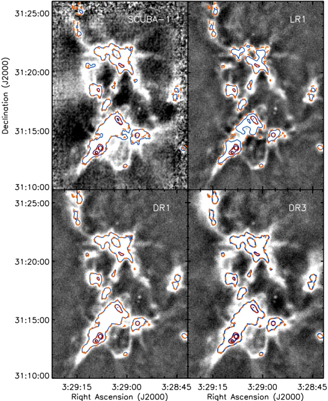
accurate measurements of emission structures on as large a scale as possible. New instrumentation, observing techniques, and data reduction tools allow for better recovery of larger-scale emission structures than was feasible in the past. As an example, Figure 1 shows the emission observed in the NGC1333 star-forming region in the Perseus molecular cloud as seen with the original SCUBA detector (Sandell & Knee 2001) compared with the same map obtained with
SCUBA-2, as part of the GBS survey, and reduced using several different techniques. The SCUBA-2 map was first presented in Chen et al. (2016)using the GBS Internal Release 1 (IR1) reduction method, but it is shown in Figure 1 using several more recent SCUBA-2 data reduction methods, all of which are discussed further throughout this paper. While bright and compact emission structures appear the same in all panels, the GBS DR3 map clearly recovers the most faint and extended
Figure 1.Comparison of emission observed in NGC1333. The top left panel shows data from SCUBA published in Sandell & Knee (2001), while the remaining three panels show SCUBA-2 observations converted into Jy beam−1
flux units assuming a 14 6 beam as in Dempsey et al. (2013). The SCUBA-2 reductions shown are the JCMT LR1 (top right), JCMT GBS DR1 (bottom left), and JCMT GBS DR3 (bottom right), all discussed further in this paper. In all panels, faint emission is emphasized in the gray scale, which ranges from −0.05 to 0.1 Jy beam−1. Both the solid blue and dashed orange contours indicate emission at 0.2, 1, and
structure while suffering the least from artificial large-scale features, such as that seen at the center left of the SCUBA image. In this paper, we focus on the reliability of the GBS SCUBA-2 maps and do not present any quantitative compar-isons with SCUBA data.
While not the focus of our present work, we note that space-based submillimeter facilities such as the Herschel Space
Telescope avoid the challenge of observing through the atmosphere and therefore offer the ability to obtain observa-tions with much less filtering. At the same time, space-based submillimeter facilities have much lower angular resolutions, due to the difficulty in placing large dishes in space. Previous work by JCMT GBS members provides a comparison of star-forming structures observed using Herschel and SCUBA-2 (Sadavoy et al. 2013; Pattle et al. 2015; Chen et al. 2016; Ward-Thompson et al. 2016), although all of these analyses used earlier SCUBA-2 data reduction methods than the methods analyzed here. The loss of larger-scale emission structures inferred by comparing SCUBA-2 and Herschel observations will therefore be somewhat less severe when the current data products are used instead.
To achieve the various science goals of the GBS, it is important to have a thorough understanding of the complete-ness and reliability of the sources detected. Uncertainties in source detection and characterization can arise from both the observations and map reconstruction efforts, as well as from the tools used to identify and characterize the emission sources. In the analysis presented here, we aim to thoroughly investigate the first of these issues, i.e., quantifying how well a source of known brightness and size is recovered in a JCMT GBS map, when an idealized source-detection algorithm is used in an ideal (noncrowded) environment.
The JCMT GBS has released several versions of ever-improving data products to the survey team for analysis—IR1, Data Release 1 (DR1),18 Data Release 2 (DR2), and Data Release 3 (DR3)—while the JCMT has also released maps of all 850 μm data obtained between 2011 February 1 and 2013 August 1 through their JCMT Legacy Release1 (LR1; S. Graves et al. 2018, in preparation; see also http://www.
eaobservatory.org/jcmt/science/archive/lr1/). Table 1
sum-marizes all currently published GBS maps. The last three GBS data releases, intended to be made fully public, are the focus of this paper. We also provide an approximate comparison of the GBS data products to the JCMT’s LR1 maps, which are qualitatively similar to the intermediate “automask” GBS data products discussed in the text.
Within the GBS data releases, DR2 improves on DR1 through the use of improved data reduction techniques that enhance the ability to faithfully recover large-scale emission structures. Many of these improvements were outlined in Mairs et al. (2015), but it was beyond the scope of that work to fully replicate the data reduction process used for DR1 and DR2 and quantify how well structure in the maps is recovered. Additionally, several small modifications to the data reduction procedure were made after the testing performed in Mairs et al. (2015). The majority of this paper focuses on a careful comparison between the recovery of structure using the exact JCMT GBS DR1 and DR2 methodologies. Unlike DR1 and DR2, DR3 does not involve a completely new re-reduction of all JCMT GBS observations with improved recipes. Instead, DR3 focuses on estimating the pointing offset errors present in the observations and adjusting the final DR2 maps to correct for them.
Quantifying the quality and fidelity of our JCMT GBS maps is a crucial step for the overarching science goals of the survey. For example, one goal is to measure the distribution of core masses and compare this distribution with the initial (stellar) mass function (Ward-Thompson et al. 2007). Without detailed knowledge of source recoverability and whether or not there is any bias in real versus observable flux, the obtained core mass function could be misinterpreted. A wide range of artificial Gaussians were used in our testing, ranging from sources that should be difficult to detect (e.g., peak brightnesses similar to the image noise level) to those that should be easy to recover accurately (e.g., compact sources with peaks at 50 times the image noise level). We emphasize that, especially for the former case, the recovery results we present here represent an unachievable ideal case for realistic analysis: knowing precisely where to look for the injected peaks, as well as precisely what to look for (known peak brightness and width), allows us to recover sources that would never be identifiable in a real observation. A full quantification of completeness would require
Table 1 GBS Published Mapsa
Region Data Version Reference DOIb
CrA DR1 D. Bresnahan et al. (2018, in preparation) Pending
Auriga DR1 Broekhoven-Fiene et al. (2018) https://doi.org/10.11570/17.0008
IC5146 DR1 Johnstone et al. (2017) https://doi.org/10.11570/17.0001
Lupus DR1 Mowat et al. (2017) https://doi.org/10.11570/17.0002
Cepheus DR1 Pattle et al. (2017) https://doi.org/10.11570/16.0002
OrionA DR1 automask Lane et al. (2016) https://doi.org/10.11570/16.0008
TaurusL1495 IR1 Ward-Thompson et al. (2016) https://doi.org/10.11570/16.0002
OrionAc DR1 Mairs et al. (2016) https://doi.org/10.11570/16.0007
Perseus IR1 Chen et al. (2016) https://doi.org/10.11570/16.0004
SerpensW40 DR1 Rumble et al. (2016) https://doi.org/10.11570/16.0006
OrionB DR1 Kirk et al. (2016) https://doi.org/10.11570/16.0003
Ophiuchus IR1 Pattle et al. (2015) https://doi.org/10.11570/15.0001
SerpensMWC297 IR1 Rumble et al. (2015) https://doi.org/10.11570/15.0002
Notes.
a
This table includes only published GBS papers where the submillimeter map was publicly released alongside the paper.
b
Digital Object Identifier is a permanent webpage where a static version of the GBS data is stored for public distribution.
c
While analysis was performed only in the southern portion of the map, the entire map is provided at the DOI.
18
This is called the “GBS Legacy Release 1” in Mairs et al. (2015).
including non-Gaussian sources (e.g., also filamentary morpholo-gies and elongated cores with non-Gaussian radial profiles), testing the effects of source crowding, testing several of the commonly used source-finding algorithms and determining the influence of false-positive detections, and not tuning the source-finding algorithm to look for emission in known locations. Such an analysis is beyond the scope of this paper, although some aspects have been examined by previous studies (e.g., Kainulainen et al.
2009; Kauffmann et al.2010; Men’shchikov 2013; Pineda et al.
2009; Rosolowsky et al. 2008, 2010; Reid et al. 2010; Shetty et al.2010; Ward et al.2012).
The paper is structured as follows. In Section2, we discuss the JCMT GBS observations and the general data reduction procedure. In Section 3, we describe our method for testing source recoverability and fidelity in source recovery in the DR1 and DR2 maps, and the results are discussed in Section 4. These tests provide essential metrics for future analyses of GBS data where the role of bias and the recoverability of real structure in the observations will need to be understood. In Section 5, we introduce two independent methods for measuring the telescope-pointing errors in each observation and demonstrate that the final DR3 maps should have little residual relative pointing error. This analysis provides us with confidence that the properties of emission structures measured in DR3 should not be substantially more blurred out than expected from the native telescope resolution.
2. Observations
SCUBA-2 observations were obtained between 2011 October 18 and 2015 January 26. Observations were made in Grade 1 (τ225 GHz<0.05) and Grade 2 (0.05<τ225 GHz<0.08) weather conditions. Grade1 weather provides good measurements at both 850 and 450 μm, while Grade2 weather is suitable for 850 μm and provides poorer measurements at 450 μm. Each field was observed four to six times, depending on the local weather conditions, to obtain approximately constant noise levels across the survey at 850 μm. Observations at 450 μm are more sensitive to the atmospheric conditions and hence show a significantly larger variation in noise properties.
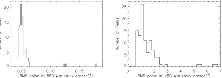
Table4summarizes the approximate noise level in each field of the survey, while Figure 2 shows the distribution of noise
levels. We ran the Starlink PICARD (Gibb et al. 2013)recipe
mapstatson each individual observation to calculate the noise in the central portion (i.e., inner circle of radius 90″) of the observed area. We then estimated the effective noise for each field in the final mosaic by accounting for the fact that the observations are combined using the mean values weighted by the inverse square of the noise at that location. For most of the paper, we focus on the 850 μm data, where the noise levels are more uniform.
The standard observing mode used for the GBS data was the PONG 1800 mode (Kackley et al.2010), which produces fully sampled 30′ diameter regions. The GBS obtained a total of 581 observations under this mode, as well as a handful of additional observations under the PONG 900 and PONG 3600 modes during SCUBA-2 science verification (SV). We focus our analysis here entirely on the PONG 1800 observations. Earlier testing by the GBS data reduction team showed that the other mapping modes have different sensitivities to large-scale structures.
We reduced the maps using the iterative routine known as
makemap, which is distributed as part of the SMURFpackage (Chapin et al. 2013a, 2013b) in Starlink (Currie et al.2014). We used a gridding size of 3″ pixels at 850 μm and 2″ pixels at 450 μm and halted iterations when the map pixels changed on average by <0.1% of the estimated map rms. In both DR1 and DR2, we reduced each observation twice, following a similar overall procedure. In the first reduction, known as the automask reduction, pixels containing real astronomical signal were estimated using various signal-to-noise ratio (S/N) criteria applied to the raw-data time stream. We then mosaicked together all maps of the same region and determined more comprehensive areas of likely real astronomical signal. These areas were then supplied as a mask for the second round of individual reductions, known as the external-mask reduction. The final mosaic was created using the output of the second round of reductions.
The final (external mask) mosaic tends to contain much more large-scale emission structure than the first (automask) mosaic. The reason for this difference is that the mapmaking algorithm needs to distinguish between larger modes of variation in the raw time stream data, which arise from scanning across true astronomical signals, versus those induced by variations in the sky or instrumental effects, which it does through the use of a mask.
Figure 2.Distribution of rms values for each field mapped by the GBS. The left panel shows the rms values at 850 μm, while the right panel shows the rms values at 450 μm. Here 1 mJy arcsec−2corresponds to approximately 242 mJy beam−1at 850 μm and 109 mJy beam−1at 450 μm. Note that the three highest rms values in
each panel correspond to science verification fields that were not observed to their full depth. The final high-noise outlier at 450 μm corresponds to one of the fields in Lupus, which was observed during marginal weather at a low elevation, conditions that adversely affect 450 μm data to a much greater extent than 850 μm.
By being able to combine four to six initially reduced maps together to determine where real astronomical signal is likely, it is possible to accurately identify emission over a much larger area of sky than is evident from the raw data in a single observation. The differences between our DR1 and DR2 procedures focused on methods of improving the sensitivity to larger-scale structure in the initial automask reduction (e.g., reducing large-scale filtering), as well as creating more generous, but still accurate, masks for the external-mask reduction (e.g., lowering the mask S/N criteria). We note that in defining the mask, there are two competing challenges, as also discussed in Mairs et al. (2015). Masks that are smaller than the true extent of the source emission will prevent a full recovery of that emission, leading to artificially smaller and fainter sources. At the same time, masks that include regions without real source emission are liable to introduce false large-scale structure, which may artificially increase the total size and brightness of real sources. Appendix A outlines the full reduction procedure and
makemapparameters applied for both DR1 and DR2.
Although not identical, the data reduction procedure for the JCMT’s LR1 data set is similar to the GBS DR1 automask procedure: only one round of reduction is run, and strong spatial filtering is applied to suppress real and artificial large-scale structures.
In DR3, we use the DR2 reductions for each observation and then search for possible offsets between observations of the same field due to telescope-pointing errors. If positional offsets are found, we apply the appropriate shift to the observation before creating the final mosaicked image. This procedure is discussed in more detail in Section 5.
One final data reduction parameter that we do not refine beyond the standard recommended procedure is the appropriate flux conversion factor (FCF) applied to each observation. As discussed in Dempsey et al. (2013), the standard observatory-derived FCF values appear stable over time, with a scatter of less than 5% at 850 μm and about 10% at 450 μm in relative calibration, while the absolute calibration factors are approximately 8% and 12% at 850 and 450 μm, respectively. The JCMT Transient Survey demon-strates that it is possible to improve the relative calibration at 850 μm to 2%–3% (Mairs et al. 2017b); however, the Transient Survey procedure requires multiple bright point sources per observation, which many GBS fields do not possess. We therefore simply note that the GBS source flux estimates should be accurate to 8% at 850 μm and 12% at 450 μm using the default calibrations, as confirmed in Mairs et al. (2017b). A small fraction of sources may also have variable emission, although most of the variable candidates identified in the Transient Survey show variations in flux of less than a few percent over the course of the typically short (days or months) time span between typical GBS observations of the same field (Mairs et al.2017a; Johnstone et al.2018). Only one source of the ∼150 monitored by the Transient Survey shows variability of more than 10% over short timescales (EC 53 in Serpens; Yoo et al.2017; Johnstone et al.2018).
For completeness, we note that where available, all GBS data releases additionally include “CO-subtracted” maps. The 12
CO(3–2) emission line lies within the 850 μm bandpass and therefore can contribute flux to the emission measured (e.g., Drabek et al. 2012). This “CO contamination” is typically <10% of the total flux measured, although it can be significantly higher (up to 80%) in rare cases where there is an outflow in a lower-density environment. Where appropriate measurements of the 12CO(3–2) integrated intensity were available to the GBS, we ran an additional round of reductions
for each of DR1, DR2, and DR3 with the CO emission properly subtracted from the 850 μm map. A brief summary of our CO subtraction procedure is given in AppendixA.4.
3. Source Recovery Measurements
Here we discuss our procedure for measuring our accuracy in recovering emission structures.
3.1. Test Setup
As discussed in Section2, Starlink’s makemap is the standard software for reducing SCUBA-2 mapping observations. Using
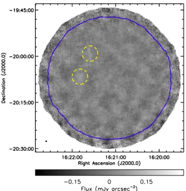
makemap, the user can insert artificial sources directly into an observation’s raw-data time stream, providing an easy mechanism to measure how well idealized model emission structures are recovered under different data reduction settings. Our approach was guided by the aim to systematically test the best-case scenario of isolated point sources that are not confused by a local background. We emphasize that many of the dense cores identified in the GBS will have some degree of crowding and/or hierarchical structures, which will reduce the reliability of the recovered emission. We used the GBS 850 μm observations of the OphScoN6 field as the basis for our testing. It is the GBS field that contains the least amount of real signal, i.e., the observation mostly closely resembling a pure-noise field. OphScoN6 was observed seven times rather than the standard six times for observations obtained in Grade2 weather, so we excluded one of the observations (20130702_00031) to make the data set more similar to a standard GBS field. This excluded observation was taken under marginal weather conditions with higher noise levels than are typical for most GBS observations. The noise at 850 μm in the mosaic of the six OphScoN6 maps is 0.049 mJy arcsec−2, which is similar to that of other GBS fields (cf. Table 4 and Figure2).
Figure 3 shows the DR2 automask reduction of the OphScoN6 data used here. A careful visual examination of the map shows that there are two faint zones of potentially real emission to the east of the field, but, with the low peak signal level, neither are definite detections. Nonetheless, we take care in our completeness testing to avoid potential biases due to low-level emission in these regions.
We generate artificial, radially symmetric Gaussian sources with a range of peak intensities and widths to add to each raw observation, to test how well they are recovered in the final reduced mosaic. We constrain all fake sources to lie in angular separation at least three Gaussian σ away from the outer 3′ of the map (where the local noise is significantly higher) and away from the zone of potential emission in the east of the mosaic, defined as two circles of 2 5 radius, with the centers set by eye. Both of these excluded map areas are shown in Figure3.
For any given set of Gaussian parameters (i.e., amplitude and width), we randomly placed 500 sources, eliminating those that landed in the edge or possible emission zones noted above or those located less than 6σ away from a previously placed source. In the case of the narrowest (σ=10″) Gaussians we tested, this process resulted in more than 100 inserted sources per map. For the widest (σ=150″) Gaussians we tested, however, only one or two sources could be placed in a map while still satisfying all of the above criteria. We therefore created multiple maps with artificial sources added for the widest Gaussians to improve our statistics. We note, however, that our statistics are still poorer for the widest Gaussian cases. It is too computationally intensive to run hundreds of
reductions for each wide Gaussian to match the number of sources able to be inserted in a single narrow Gaussian test image.19Table2
summarizes the Gaussian parameters used for testing and lists the total number of artificial sources used for each combination of width and peak. In total, we inserted 3196 artificial Gaussian sources into the maps. We explored 63 different Gaussian widths and amplitudes, with a total of 306 test fields, to boost our statistics. Figure4shows an example of the test setup with the artificial Gaussian sources added directly to the original mosaic. Since these Gaussians have not passed through our data reduction pipeline, deviations from perfect Gaussians are entirely attributable to the background noise in the mosaic.
3.2. Data Reduction
After creating each instance of artificial Gaussians, we run our standard GBS data reduction procedure with the artificial Gaussians added directly into the raw-data time stream for each of the six observations of OphScoN6 using the “fakemap” parameter in makemap. The standard reduction procedure is outlined in Section 2. We emphasize that the external mask is created separately for each set of artificial Gaussians, based on the individual automask reductions. We follow these steps for both the DR1 and DR2 reduction procedures. For each set of added artificial Gaussians, we therefore have four maps to examine: DR1
and DR2, for both the automask and external-mask reductions. Figure5shows the DR2 external-mask reductions for the four test cases from Figure 4. Comparison of these two figures reveals a clear difference in the quality of source recovery for smaller and larger sources, which will be analyzed quantitatively in Section4.
3.3. Source Recovery
We next use an automated method to determine how well the artificial Gaussians are recovered in each of the maps. In normal scientific analyses, uncertainties in where real emission is located and its true structure can complicate emission recovery. Here we take advantage of knowing precisely where the emission is located and what the brightness profile should look like to reduce the uncertainties associated with source recovery. For each known artificial Gaussian peak position, we use mpfit (Markwardt2009) to search the surrounding 3.0σ radius for a given input Gaussian size. This search window is large enough to encompass the model Gaussian peak to 0.003 times the peak brightness, which corresponds to about one-tenth of the image rms for the brightest model Gaussians. To eliminate spurious noise features being identified, we discard any fits that did not converge, had large fitting uncertainties,20were dominated by an artificial background term,21or had properties too different from the input values.22We did not eliminate sources that were much fainter or smaller than the input Gaussians, as we expect the data reduction process to create smaller and fainter sources than we started with, as shown by Mairs et al. (2015), and we wish to quantify this effect. Finally, to
Figure 3.The OphScoN6 field as observed by the JCMT GBS at 850 μm. The image shown is the external-mask reduction for DR2. Both the DR1 and DR2 reductions (automask and external mask) appear similar in this region due to the lack of structure detected. (We note that the DR2 reductions show faint large-scale mottling that is not present in the DR1 reductions, as DR1 included additional large-scale filtering outside of the masked regions. See AppendixA
for more details.) The yellow dashed circles show the approximate location of two possible faint emission structures in the map, while the blue contour shows a separation of 3′from the edge of the mosaic. The small black dot at the bottom left indicates the SCUBA-2 beam.
Table 2
Number of Gaussian Peaks Analyzed
Amplitude σ (arcsec) (Nrms) 10 30 50 75 100 125 150 1 163 50 57 36 24 14 10 2 170 45 61 37 21 20 11 3 151 52 63 37 23 16 9 5 171 48 55 42 22 19 9 7 147 53 53 37 24 20 9 10 181 45 57 37 21 16 12 15 159 45 58 34 20 19 11 20 166 48 57 35 20 15 11 50 152 52 58 37 23 17 11 Nrepeata 1 1 3 5 6 9 9 Note. a
The number of reductions run for each input Gaussian σ value, done to increase the total number of artificial sources available for analysis.
19
For reference, the reduction of each SCUBA-2 raw observation requires approximately 1.5 hr running on a dedicated 100GB RAM, 12 core CPU machine, while each test Gaussian input field uses a mosaic of six raw observations and requires four reductions (DR1 and DR2, automask and external mask).
20
Specifically, we discarded fits where the ratio of the peak flux or width and its associated fitting error was less than three, i.e., any fits where the peak flux or width was uncertain by at least 100% within the standard 3σ uncertainty range. We also excluded fits where the uncertainty in the location of the peak exceeded 50% of the input Gaussian width.
21
Small fitted background terms may be reasonable if the source lies near the peak or valley of a noise feature in the mosaic. We excluded fits where the absolute background exceeded half of the input peak flux or one-third of the fitted peak flux.
22This criterion required true source recoveries to have a peak location within
1.25σ of the true center—a radius of 1.25σ corresponds roughly to the full width at half maximum (FWHM). We also required the fits to be approximately round (axial ratios less than 1.5), have a peak no more than 2.5 times the real value, and have a width no more than twice the real value. Finally, we excluded fits that were offset from their input locations by more than the input Gaussian width divided by the square root of the peak S/N of the input Gaussian; brighter Gaussians should have more accurately determined centers.
ensure that noise spikes or underlying larger-scale structure from the original data were not contaminating our results, we performed a similar Gaussian fit on the original mosaics (i.e., maps with no artificial sources added). We then removed from our list of recovered artificial sources any fits that had consistent fit parameters to the original mosaic fit (within 1.5 times the fit uncertainty in all fit parameters). We emphasize that our entire Gaussian-fitting procedure gives the best case possible for source recovery. Many of the faintest sources that we can find in our maps would not be identifiable using a standard source-detection algorithm that was not targeted to known positions and Gaussian properties.
We note that all of our source recovery tests discussed here and in the following sections focus on the 850 μm observations. We expect that the 450 μm data would follow qualitatively similar trends but would not behave identically. Early testing by the data reduction team showed that in general, large-scale structure is better recovered when larger pixel sizes are adopted. The GBS uses smaller pixels for the 450 μm maps (2″) than the 850 μm maps (3″) to account for the smaller beam size of the former. Therefore, we expect that for structures of equal size and the same peak brightness S/Ns, recovery will be poorer in the 450 μm map.23
4. Analysis: Artificial Source Recovery
In our analysis below, we examine the final reduced mosaics to determine the effectiveness of each reduction in recovering the artificial Gaussians introduced into the raw-data time stream. The quantitative metrics that we examine are the fraction of Gaussians recovered; the recovered peak flux, total flux, and size compared with the input values; and the recovered axial ratio and offsets in the recovered peak position. We also note that our artificial source recovery gives us a tool not available for normal observations. By comparing the reduced maps with and without the artificial sources added to the raw-data time stream, we can measure precisely how much flux each artificial source contributes to the final reduced map. The analysis of the difference maps is presented in AppendixB.
4.1. Recovery Rate
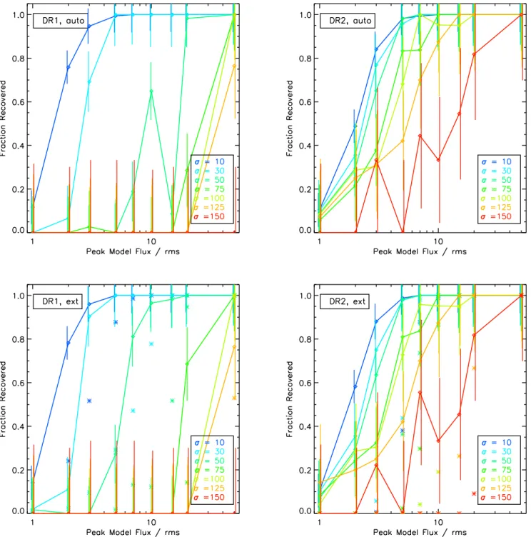
The first metric that we analyze is the recoverability of the artificial Gaussians in the final maps. We emphasize that this recovery rate is an upper limit to the detection rate that it would be possible to measure in real observations, where source properties are not known and complications such as source crowding exist. Figure 6 shows the fraction of sources recovered versus the peak flux for Gaussians of various widths using different data reduction methods. Bright and compact
Figure 4.Illustration of the artificial Gaussian test setup. The background gray-scale image shows the original OphScoN6 DR2 external-mask mosaic with the artificial random Gaussians added directly to the image. As in Figure3, the gray scale ranges from −0.3 to 0.3 mJy arcsec−2. These images represent the idealized case where the data reduction
process perfectly returns all structure in the area. The blue crosses denote the centers of each random Gaussian, while the dashed yellow circles show regions of the mosaic where the Gaussians were not allowed to be placed due to low-level potential emission structures present in the mosaic. All of the Gaussians shown have amplitudes of 10 times the mosaic rms noise. From top left to bottom right, the Gaussians have widths (σ) of [30″, 50″, 100″, 150″], respectively.
23
Source recovery testing at 450 μm is also complicated by the fact that we apply the 850 μm–based mask for the 450 μm data reduction.
sources are always recovered, regardless of the reduction method. Compact sources become poorly recovered only at extremely low intensity levels, i.e., peak amplitudes of one or two times the mosaic rms. On the other hand, extended sources are more difficult to recover. We also examine the subset of recovered sources that lie within the mask whose properties are expected to be better recovered (in the external-mask reduc-tion), as demonstrated in Mairs et al. (2015). Some of the recovered sources are only marginally brighter than the local noise level, and in many of these cases, they are sufficiently faint that they did not satisfy the masking criteria we adopted. Therefore, we find that the total source recovery rate is poorer for sources that lie within the mask, although it follows the same general trend as the full set of recovered sources (i.e., a higher recovery rate for brighter and more compact input Gaussians). The recovery rate of sources that lie within a mask is generally a better representation of the detection rate of sources that could be confidently identified in real observations; however, an important exception is that moderately bright but very compact sources may have too few pixels to satisfy the DR2 masking criteria, even though they are clearly detectable. A comparison of the DR1 (left column) and DR2 (right column) reductions in Figure 6 shows that the latter is much better at retaining larger sources in the automask and external-mask reductions. For large (σ 100″) and bright (input peaks 10× rms) input Gaussians, we typically recover at least twice
as many of the Gaussians in DR2 maps as we can in DR1 maps.
In Figure6, we also see slight improvement in the fraction of recovered sources between the automask and external-mask reductions. We generally expect the external-mask reductions to improve the reliability of recovered source properties (as examined in the following sections), rather than the recovery fraction itself. Indeed, for a source to be included in the external mask, by definition, it must be visible already in the automask reduction. Therefore, the similarity in source recovery fractions between automask and external-mask reductions is expected. We attribute the marginal difference in recovered sources in the external-mask reduction to added sources near our detection limit and do not consider the difference in source recoveries to be significant. These faint or extended Gaussians are barely distinguishable from the back-ground-map noise, even with our generous recovery criteria. As also noted in Mairs et al. (2015), the recovery rate for sources in the GBS DR1 map should therefore be similar to that of the JCMT LR1 maps, which are similar to the GBS DR1 automask reductions.
Our source recovery rates compare favorably with the JCMT Galactic Plane Survey (JPS), a JCMT legacy survey that focused on mapping 850 μm emission of large areas of the Galactic plane using the larger PONG 3600 mapping mode. Eden et al. (2017)ran a series of completeness tests, injecting
Figure 5.Examples of final mosaics using the DR2 external-mask reduction method, with the artificial Gaussians added into the raw data prior to processing. This figure shows the same artificial Gaussian fields as Figure4, with the same gray scale and other plotting conventions. The maroon triangles show the sources that were recovered within an external mask, the purple squares show the sources that were recovered outside of an external mask (i.e., are too faint to satisfy masking criteria; see Section4.2), and the red circle shows a nondetection.
artificial Gaussians of FWHM=21″ (σ∼9″) with a range of peak brightnesses, using the CUPID source-detection algorithm
FellWalker to measure their observable properties. They reported a 90%–95% detection rate for sources with peak fluxes of five or more times the noise level and did not test the detection rate for larger sources. For comparison, we recover 100% of the σ=10″sources with peak fluxes of five or more times the noise in both external-mask reductions.
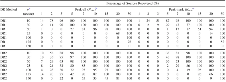
Table3 summarizes the percentage of sources recovered in each of the external-mask reductions as a function of data reduction method and input artificial Gaussian parameters. The
left-hand portion of the table provides statistics for all recovered sources, while the right-hand portion provides statistics for the subset of recovered sources within an external mask. We again emphasize that these values represent upper limits to the observable detection rate, where a blind search is run on sources with varying levels of crowding.
4.2. Recovered Properties: Peak Flux
For the artificial Gaussians that were recovered, we now examine how well their measured properties match the input
Figure 6.Fraction of artificial sources recovered in each reduction method. Top row: automask reductions for DR1 (left) and DR2 (right). Bottom row: external-mask reductions for DR1 (left) and DR2 (right). In each panel, the fraction of sources recovered is shown vs. the input source amplitude in units of the mosaic rms (0.049 mJy arcsec−2). Each color shows sources with a different input width (Gaussian σ values are shown in the legend at the bottom right, in arcseconds). The error
bars denote the Poisson error for each input Gaussian test case (the square root of the number of input Gaussians). The diamonds denote all recovered sources, while the asterisks denote recovered sources that lie within the external mask (bottom panels only).
properties. We measure the mean and standard deviation of the recovered Gaussian-fit values and compare them to the input Gaussian values. Table 5 summarizes the recovered Gaussian properties for each of the external-mask reductions. For each reduced map, we report on the mean and standard deviation of the fraction of the measured Gaussian property with the initial input value. Table5includes the peak flux (discussed here), as well as the Gaussian width σ and the total flux (discussed in the following sections).
Figure7 shows how well the peak flux is recovered for all recovered sources. For the faintest input Gaussians, the recovered peak flux is typically larger than the input value; i.e., the peak flux ratio is above one. Faint artificial sources with peak fluxes near the typical noise level in the map (one or two times the rms) are easier to recover when these sources are coincident with positive noise features in the map. We therefore expect the recovered faintest peaks to have peak fluxes biased toward higher values. Eden et al. (2017) reported a similar behavior for their completeness testing in the JPS maps. The black dashed curve in Figure7shows the approximate effect of this bias by showing a measurement of a peak flux equal to the local rms. While not identical, the shape of this curve gives a reasonable approximation of the measured peak flux ratios at low input peak flux values for DR2.
Figure7also shows that the peak fluxes are better recovered for compact sources than larger sources. Larger sources have a great fraction of their flux at larger size scales and are thus expected to be more sensitive to filtering. We constructed a simple model of the large-scale spatial filtering that occurs during data reduction to see how well it predicts the observed source recovery behavior. Accordingly, we created a series of two-dimensional Gaussian models matching our artificial Gaussian sources. We approximated the filtering as a single-scale boxcar-smoothed version of the model being subtracted from the original. We fit the resulting filtered model with a two-dimensional Gaussian (including a constant zero-point term to
alleviate fitting challenges with slight negative bowling) to calculate the fractional reduction in peak flux and size.
Previous tests of the initial data reduction method employed by the GBS (IR1, not examined here) suggested that source recovery was consistent with a simple single filtering scale of about 1′. The subsequent data reduction methods examined here (DR1 and DR2) were expected to recover more emission, i.e., be described by a larger filtering scale. Our test results confirm the larger scale of filtering, although we also find that a single filter scale is insufficient to describe the recovered source properties for the full range of artificial Gaussians tested. Figure7shows the predictions for the recovered peak flux ratio for a filter scale of 600″ (dotted horizontal lines). This filter scale is equal to the large-scale filtering formally applied during data reduction via the flt.filt_edge_largescale=600 parameter. Peak flux ratios lying below the model line imply they have been subject to more filtering than in the model, i.e., filtering on a smaller size scale. The 600″ filtering scale matches the smallest artificial Gaussian sources, of sizes of below about 75″ for the external-mask reduction of DR2; i.e., the dashed filtering model curves are a good match for the recovered peak flux ratios at the highest S/N values. At the same time, the model clearly underpredicts the amount of filtering for larger sources for that same reduction.
Comparing the reductions, Figure7clearly shows that DR2 recovers more reliable peak flux values than DR1. Also, although the difference is subtle, the external-mask reductions improve on the automask reductions, especially for the largest and brightest of input Gaussians. In cases where not all of the recovered sources lie within the external mask, the subset of sources that are included in the mask tend to have recovered peak fluxes that more closely correspond to the input value than the full sample of sources do. As an example, in DR2, a Gaussian with σ=100″ and a peak flux of 10 times the noise has recovered peak fluxes of about 37% of their true value in the automask reduction, while this rises to roughly 40% of their
Table 3
Source Recovery for External-mask Reductions Percentage of Sources Recovered (%)
DR Method σa Peak-all (Nrms)b Peak-mask (Nrms)c
(arcsec) 1 2 3 5 7 10 15 20 50 1 2 3 5 7 10 15 20 50 DR1 10 14 78 96 100 100 100 100 100 100 1 24 51 87 98 100 100 100 100 DR1 30 2 11 90 100 100 100 100 100 100 0 2 9 29 47 77 100 100 100 DR1 50 1 0 0 27 81 96 98 100 100 0 0 0 1 13 12 51 94 100 DR1 75 0 0 0 0 0 0 0 68 100 0 0 0 0 0 0 0 14 100 DR1 100 0 0 0 0 0 0 0 0 100 0 0 0 0 0 0 0 0 100 DR1 125 0 0 0 0 0 0 0 0 76 0 0 0 0 0 0 0 0 52 DR1 150 0 0 0 0 0 0 0 0 0 0 0 0 0 0 0 0 0 0 DR2 10 10 58 88 98 100 100 100 100 100 0 0 0 38 87 98 100 100 100 DR2 30 10 35 75 97 100 100 100 100 100 0 0 5 43 98 100 100 100 100 DR2 50 7 29 63 98 100 100 100 100 100 0 0 0 36 73 100 100 100 100 DR2 75 8 24 32 80 83 100 100 100 100 0 0 0 2 29 86 100 100 100 DR2 100 4 28 30 72 95 95 95 100 100 0 0 0 0 4 19 95 100 100 DR2 125 14 20 25 42 70 87 100 100 100 0 0 0 0 0 0 26 66 100 DR2 150 0 0 22 0 55 33 45 81 100 0 0 0 0 0 0 0 9 100 Notes. a
The Gaussian width, σ, of the inserted artificial Gaussians.
b
The peak flux of the inserted artificial Gaussians, given in units of the rms noise of the map. The source recovery fractions listed in these columns give all of the recoveries within the map.
c
The peak flux of the inserted artificial Gaussians, given in units of the rms noise of the map. The source recovery fractions listed in these columns give only the recoveries that lie within the external mask.
true value in the external-mask reduction for all sources and 43% for those lying within the mask. In contrast, no sources are reliably recovered in either the automask or external-mask reduction of DR1 for these Gaussian properties. As noted in Mairs et al. (2015), sources are only accurately recovered in the external-mask reductions when the mask encompasses the true extent of the source. The superiority of the DR2 reductions over the DR1 reductions is therefore partly attributable to the mask-making procedures, which better reflect the true source extents in DR2 than in DR1.
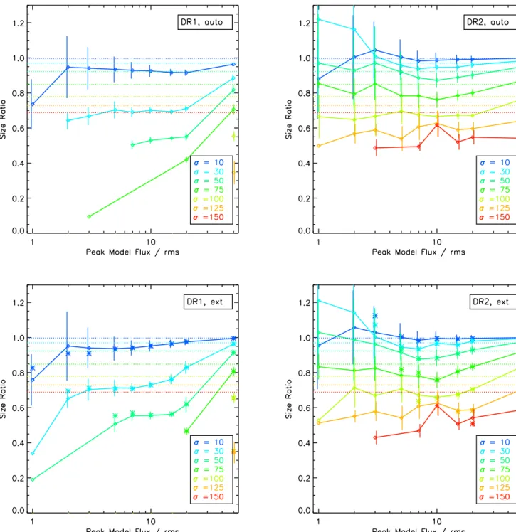
4.3. Recovered Properties: Sizes
Figure 8 shows the size ratios measured for the artificial Gaussians. We remind the reader that the input Gaussians were all round, though we allowed fits for sources with axial ratios up to 1.5:1 (Section3.3). We present here a single size estimate based on the geometric mean of the two Gaussian σ values. In general, we find similar results to those previously presented: (1) compact and brighter Gaussians have their sizes recovered more accurately, (2) DR2 tends to show more reliable
Figure 7.Peak brightnesses measured for the recovered artificial Gaussian sources as a fraction of their input values. As in Figure6, the four panels show the automask (top panels) and external-mask (bottom panels) reductions using the GBS DR1 procedure (left panels) and DR2 procedure (right panels). The horizontal axis indicates the different input peak values tested, while the colors indicate the different Gaussian widths tested. The error bars indicate the standard deviation in values measured for each set of Gaussians. The black dashed line indicates the expected peak flux values where the recovered peak has a value of the local rms noise. The dotted horizontal colored lines represent model values for 600″ filtering. Diamonds denote values for all recovered sources, while asterisks denote values for sources lying within the mask (for the external-mask reduction only). See the text for details.
structures than DR1, and (3) the external-mask reduction is an improvement over the automask reduction, particularly for sources that lie within a masked area. Using a single size to describe the recovered sources is reasonable, as they tend to be quite round, with mean axial ratios of no more than ∼1.4:1 for any of the reductions. For sources that are bright or recovered within a mask (or both), the mean axial ratio is almost always lower than 1.2:1, and the sources recovered in the DR2 reduction furthermore tend to have lower axial ratios than those in the corresponding DR1 reduction.
As in Figure7, we also consider the effects of filtering on the model Gaussians. The dashed lines in Figure8 show the ratio of the mean measured filtered size to the input size for the grid of model Gaussians with which we applied a 600″ filter (see previous section for details). As expected, these models show that the more extended model Gaussians have a greater reduction in size than their more compact counterparts. The filtering model approximately predicts the size ratio for sources smaller than 50″ (blue points and lines) but underpredicts the amount of filtering for the largest sources (i.e., predicts size ratios that are too large).
4.4. Total Flux
Here we present results for the total flux recovered. For individual recovered cores, the trends discussed in the previous two sections (for peak flux and size) are at work. Figure 9
shows the total flux recovered. The values shown in this plot and Table 5 should be considered when analyzing dense core mass functions in GBS data. For compact sources (σ30″) that are brighter than 3 times the local noise, the total fluxes are recovered to better than 25% in DR2.
4.5. Location
We also examined the positional offset of the center of the recovered Gaussian compared with its true input location (not shown). Since the central location is expected to become less certain as the input Gaussian becomes larger, we measured the ratio of the positional offset to the input Gaussian width, σ. Using this measure, we find that the offset ratios are typically small, with mean values of 0.3, i.e., offsets of no more than 30% of σ, with significantly lower values obtained for model peaks of 10 or more times the rms. For the DR2 external-mask reductions, for cases where the model peak is 10 or more times the rms, the mean offset ratio is 0.05 for all input σ. For σ=30″, this implies a typical positional accuracy of better than 1 5. We therefore find that the data reduction and source recovery processes do not typically induce significant shifts to the true source positions.
4.6. Summary
Our artificial source recovery tests confirm that the GBS maps more reliably reproduce true sky emission using the newer DR2 method than the earlier DR1 method, and that using the two-step reduction process of automask reductions, mask creation, and external-mask reductions also provides improvements over a single automask reduction, particularly for bright extended sources. Sources with σ100″ are generally not recovered well, with peak fluxes and sizes often recovered at values of less than half of their true values, especially for fainter sources. Compact sources, however, are well recovered. For sources with σ30″, peak fluxes and sizes are nearly always recovered at better than 90% of
their true value for the DR2 external-mask reduction. These compact scales are of the greatest interest to the GBS, as they represent the typical scales of dense cores. We note that analyses of dense cores often discuss their sizes in terms of FWHM values instead of Gaussian σ widths; a core with σ=30″ has a corresponding FWHM of 71″. Within the Gould Belt, where clouds are between ∼100 and 500 pc, 71″ corresponds to a physical size of 0.03–0.17 pc.
For measurements such as the core mass function, where only compact structures are being analyzed, we expect that only slight corrections to the measured fluxes and sizes will be needed for cores recovered with peak fluxes between 3 and 10 times the noise in the map when using the DR2 external-mask reduction.24 For analyses using the DR1 external-mask reduction, more caution is needed if a significant number of the cores have sizes closer to σ=30″, although those with sizes closer to σ=10″ are still very well recovered. Users of the JCMT LR1 catalog (which is produced by the JCMT directly, rather than the GBS) should take note that sources detected in that catalog will have significantly underestimated peak fluxes, total fluxes, and sizes.25 The GBS DR1 automask reduction results provide an approximate guide to the level of under-estimation in each of these source properties.
In Table5, we summarize the peak flux ratios and size ratio data shown in Figures 7 and 8 so that accurate completeness can be estimated for future core-population studies. We emphasize that even for analyses of relatively compact sources using the DR2 external-mask reduction, extra attention should be paid to three factors. First, the population of sources near the completeness limit (peak fluxes of 3–5 times the noise) likely have contributions from even fainter sources (peak fluxes of 1–2 times the noise) that have been boosted to higher fluxes through noise spikes, etc. If the true underlying source population is expected to increase with decreasing peak flux, then this contribution of fainter sources could be significant. Second, faint compact sources could be either intrinsically faint and compact or brighter and larger sources that are not fully recovered. Examination of the size distribution of the brighter sources in the map should help determine what the expected properties of the fainter sources are. Third, for analyses where the source-detection rate is important (e.g., applying correc-tions to an observed core mass function), the source recovery rates presented in Section4.1should not be blindly applied, as they do not include factors such as crowding or the limitations of core-finding algorithms running without prior knowledge on a map, both of which are expected to decrease the real observational detection rate. Furthermore, while the results presented here are uncontaminated by false-positive detections, such complications will need to be carefully considered when running source-identification algorithms on real observations.
5. Further Refinements—Telescope-pointing Offsets For our final data release (DR3), we correct for telescope-pointing errors using the same reduction strategy for individual observations as in DR2. We emphasize that the completeness tests in Section 4 inject the artificial Gaussian sources at the same pixel position on every stacked map, so they are always perfectly aligned. Hence, the results from DR2 discussed in 24
At least in the absence of significant source crowding.
25
The goal of the JCMT LR1 catalog is to identify where peaks of emission exist, not to provide an accurate estimate of the total flux present.
Section 4 also apply to DR3, in both cases reflecting the properties of the sources in the coadded map. For astronomical sources in DR2 (as well as DR1), the measured properties will be artificially broadened and weakened slightly by the map misalignments. We quantify and correct for these map alignments in DR3, as discussed in this section.
Recently, the JCMT Transient Survey (Herczeg et al.2017) investigated methods to calibrate SCUBA-2 data at high precision to increase their sensitivity to small variations in flux within protostellar cores. One facet included in their calibration is telescope-pointing errors, which can often be in the range of 2″–6″. The Transient Survey has been able to decrease this error to <1″ for their final maps (Mairs et al.2017b). Indeed, pointing errors of several arcseconds could be large enough to
influence the sizes and peak fluxes of the dense cores we identify in the GBS, especially at 450 μm. Therefore, we investigated two independent methods to improve the posi-tional accuracy of our observations. Directly adopting the exact method used by the Transient team is not possible for the GBS. For example, the Transient method requires multiple bright, compact sources in their fields to estimate relative positions, whereas the GBS requires a method that will supply good absolute positions for fields that may not contain many bright compact sources.
5.1. Absolute Positions
To obtain good absolute positional accuracy, we first implement a modification of the Transient Survey method.
Figure 8.Sizes measured for the recovered artificial Gaussian sources as a fraction of the input values. See Figure7for the plotting conventions used. The Astrophysical Journal Supplement Series,238:8 (29pp), 2018 September Kirk et al.
The Transient team uses its first observation of each region as the template from which to measure all subsequent image offsets (Mairs et al.2017b). If the first observation has a large associated pointing error, however, all subsequent observations will be corrected to the wrong position.26This approach could lead to additional deficiencies for the GBS, however, since mosaics could then have blurred structures in areas of overlap between adjacent maps. Instead, we assume that, on average, pointing errors for a given field are small. While individual observations may have errors, the mosaic of all observations
(four to six per field) should be relatively more accurate. We therefore adopt the GBS DR2 mosaics as our reference template by which we align individual observations. In our final pointing-corrected mosaics, we do not see any evidence of source blurring in field-overlap areas, suggesting that this approach was reasonable.
5.1.1. Method 1: Gaussian Fits
The first alignment method that we tested follows a similar procedure to that adopted by the Transient team (Mairs et al.
2017b). There, Mairs et al. (2017b) fit bright and compact
emission in each 850 μm observation with Gaussians using the Starlink command gaussfit (part of theCUPIDpackage; Stutzki
Figure 9.Total fluxes recovered for the artificial Gaussian sources as a fraction of the input values. See Figure7for the plotting conventions used.
26
The Transient Survey is primarily concerned with relative offsets and does not contain adjacent observing areas for mosaicking, so this issue is not a problem for it.
& Guesten 1990; Berry et al. 2007). The relative offsets between Gaussian peaks in each observation of the same field were then used to estimate the overall pointing offset in that observation. Note that since the 850 and 450 μm observations are obtained simultaneously, pointing offsets derived using the 850 μm data should also be applicable at 450 μm, where the S/N is usually lower.
We followed a similar basic approach to that of Mairs et al.
(2017b). We relaxed some criteria, however, such as the
minimum peak brightness, to apply the method to a greater fraction of the GBS data. In detail, we first cropped each 850 μm image to a radius of 1200″to reduce the influence of noisy edge pixels in our later analysis. We then created a mosaic of each region and fit Gaussians to all of the peaks therein, discarding any that lay below 0.3 mJy arcsec−2
, which is slightly less than 10 times the noise for most areas of the mosaic. We also discarded any peaks from features with sizes larger than σ=40″ in either axis, as larger-scale structures are less likely to yield reliable central positions that are stable from observation to observation. This set of Gaussian fits serves as the reference to which individual observations were then compared.
For each individual observation, we first smoothed the map by 6″ to reduce pixel-to-pixel noise (using the same smoothing kernel as in Mairs et al. 2017b). Next, we fitted Gaussians to all peaks in the individual observation that lay above 0.5 mJy arcsec−2
, which is slightly less than 10 times the noise for most individual observations.27We then searched for peaks in the individual observation that were less than 10″offset from a peak in the mosaic and also had similar peak fluxes (i.e., within a factor of two).28 Our best estimate of the pointing offset for the individual observation was made by taking the median of all individual peak offset measures (separately in R.A. and decl.). For observations with three or more individual peak offset measures, we additionally removed any individual offset measures that differed by more than one standard deviation from the median of the full sample before making our final measurement of the bulk offset value.29
Our implementation of Gaussian fitting to identify pointing offsets in observations is thus conceptually similar to that used in Mairs et al. (2017b), but it allows estimates to be made in cases with many fewer and fainter peaks than are present in any of the fields covered by the Transient Survey. Our relaxed criteria could also allow spurious offsets to be measured in some cases. For example, without any additional constraints, some observations may be aligned based on a Gaussian fit to only one or two faint peaks and therefore are strongly susceptible to a variety of sources of error. Nonetheless, we generally found visually satisfactory results using this method. As discussed in the following section, however, we chose to adopt a different method, which is applicable to a broader swath of the GBS observations and appears to be slightly more reliable.
Figure10 (left panel) shows the pointing offsets estimated using the Gaussian-fitting technique. Of the 581 GBS observations, 115 did not fit our relaxed criteria, and no offsets could be measured. Of the remaining 466 observations, the full range of offsets measured in R.A. and decl. ran between −7 8 and 8 2 (with similar minima and maxima for each of R.A. and decl.), with a standard deviation of 1 9 and 2 0 in R.A. and decl., respectively. The distribution of offsets is centered on zero, with mean offsets of <0 2 in both R.A. and decl. A notable fraction of the observations showed significant offsets: 214 (46%) had total offsets 2″, 111 (24%) had total offsets 3″, and 33 (7%) had total offsets 5″.
5.1.2. Method 2:align2d
The second method that we tested involved using Starlink’s
align2d command (part of the KAPPA package; Currie & Berry 2014), which compares all pixels with significant emission in both the observation and reference mosaic to determine an optimal offset. We assumed that the two maps differed only by a simple constant offset and did not include more complex terms such as rotation or shear (as was also assumed for the previous method). We first slightly smoothed the observation (by 2 pixels using KAPPA’s gausmooth command), as we found that this improved the reliability of the offsets measured compared to the offsets measured using unsmoothed observations. We also tested a range of thresholds for pixels to use in the align2d calculation and found that the recommended setting of corlimit=0.7 worked best.30 Limiting the calculation to fewer, more reliable pixels resulted in align2d failing to measure an offset in more cases, while those that were measured tended to be consistent between corlimit values, with typical variations of less than 1 pixel (3″).
The right-hand panel of Figure 10 shows the offsets measured by align2d for all of our GBS fields. Of the 581 GBS observations, align2d was unable to measure offsets in only 29 of them, compared with 115 observations without measurable offsets using the Gaussian-fit method. None of the 29 observations had good Gaussian fits (i.e., fits where the offset is larger than the estimated uncertainty), and 22 of the 29 observations had no Gaussian fit due to insufficient emission features in their respective maps. In a few cases, however, brighter emission was present but did not yield a single consistent offset value. In these cases, multiple (usually two) peaks were identified by the Gaussian-fit method, but the offsets derived from each peak were mutually inconsistent. The sparse nature of the emission structures in these exceptional cases prevents any conclusion from being made on the cause of the inconsistency in offsets.
For the few observations where our implementation of
align2dfailed to calculate an offset, we attempted to calculate offset values that would be derived under a variety of different implementations of align2d using different values of the corlimit parameter or an unsmoothed observation. Some-times these variations in align2d did yield offset values; however, neither the magnitude nor the sign of the derived offsets were consistent between the different methods, again suggesting that simple linear offsets may not be appropriate for these particular observations.
27For comparison, Mairs et al. (2017b
)required peaks to be brighter than 200 mJy beam−1, or 0.83 mJy arcsec−2, assuming a 14 6 effective beam size,
as in Dempsey et al. (2013).
28
Mairs et al. (2017b)also required a positional coincidence of <10″ but not the additional peak flux criterion, since their matches were restricted to high-S/N peaks.
29
Mairs et al. (2017b)adopted a slightly different approach here, using the mean offset and removing any individual measures that differ by more than 4″from other measures.
30
The corlimit parameter can be varied between 0 and 1, with larger values causing more pixels to be excluded from the calculation.
Using the implementation of align2d described above, the full range of pointing offsets runs between −9 7 and 7 6 (considering R.A. and decl. separately; both span a similar range). The standard deviation of the pointing offsets is 1 7 for R.A. and 1 8 for decl. considered separately. As can be seen from Figure10(right panel), despite most observations having small pointing offsets, a nonnegligible number of fields have significant pointing errors. We find that 194, or 35%, have total offsets of more than 2″, and 86, or 16%, have total offsets of more than 3″, corresponding to the pixel size for the 450 and 850 μm maps, respectively. Eighteen maps, or about 3.3%, have total offsets in excess of 5″, which is a significant fraction of the 9 8 450 μm beam.
In Figure 11, we show a comparison of all of the offsets measured using both the Gaussian-fit and align2d methods. Clearly, the vast majority of offsets are in good agreement using either method. We carefully visually examined the few observations where align2d and the Gaussian-fit method disagree by more than 3″ (1 pixel at 850 μm, or about one-third of the 450 μm beam) and found that the align2d offset typically appeared to be the more correct of the two measures. None of the observations with discrepant derived offsets
contained many bright compact sources, where the Gaussian-fit method is expected to perform its best. We therefore adopt the
align2dmethod for DR3.
5.2. Impact on Mosaics
In most fields, many, if not all, of the observations have positions that are corrected by less than 3″, and thus the improvement in the DR3 mosaic over the DR2 mosaic is subtle. There are a handful of fields, however, where the pointing offsets are larger, and the improvement in the final mosaic is more obvious. The one (and only) dramatic example of this is the B1-S field within the PerseusWest mosaic, where pointing offsets for the six observations comprising this field range from −9 0 to 3 9 in R.A. and −9 7 to 1 0 in decl. Figure12shows a comparison of the brightest core in the B1-S field, illustrating the extreme elongation and blurring of the core seen in the DR2 map even at 850 μm. We emphasize that the B1-S field is an extreme outlier in terms of telescope-pointing errors present in the original observations, but it does serve as a good exemplar of how our pointing offset correction is effective. In all other fields, the improvement is subtle at best at 850 μm and is still minor at 450 μm. Because these offset
Figure 10.Pointing offsets derived for all GBS observations using the Gaussian-fit method (left) and align2d method (right). The solid black histogram shows offsets in R.A., while the dotted red histogram shows offsets in decl. Observations where the method was unable to be applied, e.g., due to insufficient flux in the map, are excluded. The blue dashed curve shows a Gaussian with σ=1 6 (left) and 1 7 (right) for reference.
Figure 11.Offsets derived for all GBS observations using align2d and Gaussian fitting. The left and middle panels compare the offsets derived in R.A. (left) and decl. (middle) for the two methods. Here the red dotted line shows a one-to-one relationship, while the yellow dotted lines show discrepancies of 3″(1 pixel at 850 μm) between the two measures. Offsets of zero are assigned to the relatively few observations where the method was unable to determine a measurement. The right panel shows the difference in offsets (align2d minus Gaussian) measured in R.A. and decl. Here only observations for which offsets were measured using both methods were included.