Analysis of walking and balancing models actuated and controlled by ankles

Analysis of Walking and Balancing Models

Actuated and Controlled by Ankles

by

Jooeun Ahn

B.S. Mechanical Engineering

Seoul National University, 2001

Submitted to the Department of Mechanical Engineering

in Partial Fulfillment of the Requirement for the Degree of

Master of Science in Mechanical Engineering

at the

Massachusetts Institute of Technology

September 2006

0 2006 Massachusetts Institute of Technology. All rights reserved.

The author hereby grants to MIT permission to reproduce and to

distribute publicly paper and electronic copies of this thesis document in whole or in part

in any medium now known or hereafter created.

Signature of Author...

C ertified by ...

Professor of Mechanical Engineering and

Accepted by...

Department of Mechanical Engineering

August 7, 2006

lie Hogan

Professor of Brai and Cogn ive Sciences

f,/

Thesis Supervisor

. . . .

Lallit Anand

Chairman, Department Committee on Graduate Students

AASSACHUSETTS INS TIIUE,

OF TECHNOLOGY

JAN

2 3 2007

Analysis of Walking and Balancing Models

Actuated and Controlled by Ankles

by

Jooeun Ahn

Submitted to the Department of Mechanical Engineering

on August 11 2006, in partial fulfillment of the requirements

for the degree of Master of Science in Mechanical Engineering

Abstract

Experimental data show that ankle torque is the most important actuator in normal human

locomotion.

I investigate the dynamics of simple models actuated by ankles alone. To

assess the contribution of ankle actuation to locomotion, I first analyze the dynamics of

some passive walkers without any joint torque.

These passive walkers include a rimless

wheel model and springy-legged models with and without a double stance phase.

I

analyze the stability of the period-one gait of each passive walker to compare it with the

stability of the period-one gait of an ankle actuated model.

Subsequently, I investigate

whether balancing of a double inverted pendulum model whose shape and mass distribution

are similar to a human can be achieved by control of ankle torque in a frontal plane. I

study the dynamics of the model and design a controller that makes the model balance with

biologically realistic ankle torque and a reasonable foot-floor friction coefficient.

I

conclude that an ankle-actuated model can make a stable period-one gait in a sagittal plane.

Also, I deduce that the ankle torque control in a frontal plane can stabilize a double inverted

pendulum model whose shape and mechanical properties are similar to those of humans.

Thesis Supervisor: Neville Hogan

Title: Professor of Mechanical Engineering and Professor of Brain and Cognitive Sciences

Acknowledgements

First and foremost, I express my deepest gratitude to my advisor, Professor Neville Hogan. He has given me key advice on how to start my own study. He has also given me detailed advice to improve the way how I develop my argument. All his advice has made it possible for me to

make the first step in my field.

Much thanks also to everyone in the Newman Laboratory. In particular, I would like to express a lot of thanks to Doctor Hermano Igo Krebs. He has pointed out important questions to be clarified and encouraged me to do my work with great pleasure. I also owe much thanks to

Steven Knight Charles who helped me most to accustom myself to the new environment. Also, my thanks go to Anindo Roy, Josh Young and Laura DiPietro who supported me by giving advice or encouragement. I also want to mention Shelly Levy-Tzedek, Ryan A Griffin, Nevan Hanumara,

Lorenzo Masia, and Marjorie A. Joss who helped me kindly to join the amazing laboratory.

I must mention two friends of mine. Jaehyung and Yoonhwan's friendship during the last winter has supported me so that I can regenerate myself to make my first step. I give my thanks to

them for being my constant supporters.

Last, but definitely not least, my family has been the most significant source of love and encouragement. I thank my parents, my lovely wife and my sister for their incredible support.

Also, warm hearted affections from my father in law and mother in law have supported me. Words cannot begin to explain my gratitude and love for all of my family.

Contents

A cknow ledgem ents...

3

C ontents...

4

List of Figures ...

8

List of Tables...11

1.

Introduction ...

12

1.1. M otivation and Goals... 12

1.2. Thesis Organization by Chapters ... 14

1.3. Term inology and Notation ... 15

1.3.1. A Stride Function and a Poincar6 M ap... 15

1.3.2. Vector Notation... 16

1.3.3. Time Notation... 16

1.3.4. Notation for M aps and Evolution Rules ... 17

1.4. M ethod of Stability Analysis ... 17

1.4.1. Poincard Section and the Reduced State Vector ... 17

1.4.2. Stability and Asymptotic Stability ... 19

1.4.3. Stability Analysis Using Linearization ... 19

2. A R im less W heel M odel in a Vertical Plane ... 21

2.1. Analysis of the M odel on a Horizontal Floor ... 21

2.1.1. Assumptions and Definitions of Parameters... 21

2.1.2. Analysis of Speed of the Point M ass ... 22

2.1.3. Further Analysis... 27

2.2. Analysis of the M odel on a Slight Slope ... 29

2.2.1. Assumptions and Definitions of Parameters... 29

2.2.2. Analysis of Speed of the Point M ass ... 30

2.2.3. Existence of a Period-One Gait ... 34

2.2.4. Stability Analysis of the Period-One Gait ... 35

2.3. Summary and Discussion... 42

3. A Springy Legged Model without Double Stance ... 43

3.2. Equations of M otion and Initial Conditions... 44

3.3. The Existence of a Period-One Gait ... 47

3.3.1. The Poincar6 Section ... 48

3.3.2. Algorithm for Finding Fixed Points of the Poincard M ap... 48

3.3.3. The Fixed Point of the Poincard M ap... 50

3.4. Stability of the Fixed Point of Period-One Gait... 53

3.4.1. Constructing the Poincar6 M ap ... 54

3.4.2. Stability Analysis ... 57

3.5. Sum mary and Discussion... 58

4.

A Springy Legged M odel w ith D ouble Stance...

60

4.1. Assum ptions and Definitions of Parameters... 60

4.2. Equations of M otion and Initial Conditions... 61

4.2.1. Double Stance Phase... 62

4.2.2. Single Stance Phase ... 64

4.3. The Existence of a Period-One Gait ... 66

4.3.1. The Poincard Section ... 67

4.3.2. Algorithm for Finding Fixed Points of the Poincard M ap... 68

4.3.3. The Fixed Point of the Poincard M ap... 70

4.4. Stability of the Fixed Point of Period-One Gait... 74

4.4.1. Constructing the Poincard M ap ... 74

4.4.2. Stability Analysis... 79

4.5. Analysis of the Contribution of Double Stance to Stability... 81

4.6. Summary and Discussion... 83

5. An A nkle A ctuated M odel in a Vertical Plane...

84

5.1. Assum ptions and Definitions of Parameters... 84

5.2. Equations of M otion ... 86

5.2.1. Double Stance Phase... 87

5.2.2. Single Stance Phase ... 91

5.3. Ground Reaction Forces ... 92

5.3.1. Ground Reaction Forces during Double Stance Phase ... 92

5.3.2. Ground Reaction Forces during Single Stance Phase... 93

5.5. Poincard M ap and Stability Analysis ... 99

5.5.1. Constructing the Poincar6 M ap ... 100

5.5.2. Stability A nalysis... 103

5.6. D iscussion and Future W ork... 106

5.6.1. D iscussion... 106

5.6.2. Future W ork ... 106

6.

Balancing Using Ankle Torque in a Frontal Plane ...

108

6.1. A ssum ptions and Definitions of Param eters... 109

6.2. Equations of M otion ... 111

6.3. Linearization ... 115

6.3.1. Selection of the Point about W hich Linearization is Perform ed... 115

6.3.2. Linearization about the Fixed Point... 121

6.4. Controller Design... 122

6.4.1. Block D iagram ... 123

6.4.2. A ssum ptions Regarding the Sensor and Actuator ... 123

6.4.3. Controller Design ... 125

6.5. Results from Sim ulation ... 128

6.5.1. Tim e Response of State Variables... 128

6.5.2. Time Response of the Ankle Torque and Ground Reaction Forces... 131

6.5.3. Friction Coefficient... 133

6.5.4. FurtherA nalysis... 133

6.6. Frontal Plane A nkle Torque of a W alking M odel ... 138

6.7. D iscussion and Future W ork... 140

6.7.1. D iscussion... 140

6.7.2. Future W ork ... 141

7. C onclusions ... 142

7.1. Sum m ary ... 142

7.2. D iscussion and Im plications... 144

7.3. Future W ork ... 146

A ppendix ... 149

A . Existence of Derivative M atrices of the Poincard M aps... 149

A .2. Springy legged m odels ... 151

B. Source Codes ... 153

B. 1. A Rim less W heel M odel in a Vertical Plane... 153

B.2. A Springy Legged M odel w ithout Double Stance ... 156

B.3. A Springy Legged M odel with Double Stance ... 162

B.4. An Ankle Actuated M odel in a Vertical Plane ... 172

B.5. Balancing Using Ankle Torque in a Frontal Plane ... 176

List of Figures

Figure 1-1: A schematic explanation of Poincard section... 18

Figure 2-1: A rimless wheel model on a horizontal floor; a is the initial value of 0 ... 22

Figure 2-2 : The motion of the rimless wheel; a collision occurs at point B... 22

Figure 2-3: The free body diagram of the rimless wheel at a collision ... 24

Figure 2-4: The free body diagram of the rimless wheel between collisions... 25

Figure 2-5: The vector components in the normal and the tangential directions ... 26

Figure 2-6: The rim less wheel m odel with a = n/4 ... 28

Figure 2-7: A rimless wheel model on a slight slope; y is the slope angle ... 29

Figure 2-8: The free body diagram of the rimless wheel on a slope between collisions... 31

Figure 2-9: The rimless wheel on a slope at the beginning and at the ending of a step ... 34

Figure 2-10: Asymptotic stability of the period-one gait of the rimless wheel on a slight slope ... 41

Figure 3-1: A springy legged model without double stance phase on a horizontal floor ... 43

Figure 3-2: The free body diagram of the springy legged model without double stance... 44

Figure 3-3: The initial position and velocity of the springy legged model without double stance.... 46

Figure 3-4: A position vector expressed in radial and transverse components... 46

Figure 3-5: The state of the springy legged model at t = Tf for a period-one gait... 50

Figure 3-6: The state variables during one step with vo = 1.7375 (m/s) and

P

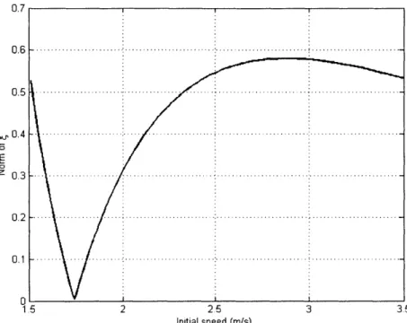
Figure 3-7: The norm of 4 with various initial speeds; initial speed varies from 1.5 to 31.5 (m/s)... 52

Figure 3-8: The norm of 4 with various initial speeds; magnified view around vo = 1.7375 (m/s)... 53

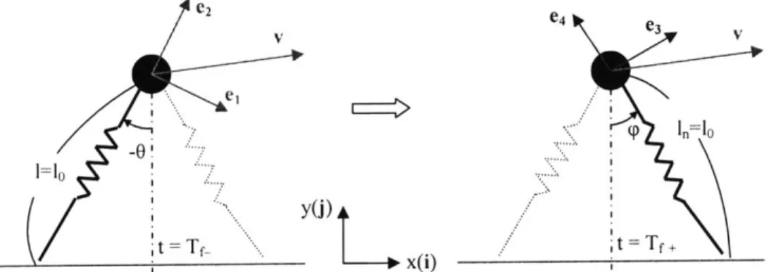
Figure 3-9: Continuity of velocity between the end of a step and the beginning of the next step. ... 55

Figure 3-10: Instability of a period-one gait of the springy legged model without double stance.... 58

Figure 4-1: A springy legged model with double stance phase on a horizontal floor ... 61

Figure 4-2: The initial position and velocity of the springy legged model with double stance...64

Figure 4-3: A position vector expressed in radial and transverse components... 64

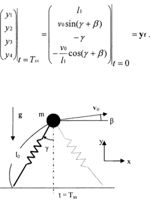
Figure 4-4: The state of the springy legged model at t = Ts, for a period-one gait... 69

Figure 4-5: The state variables during one step with vo = 2.5465 (m/s) and

P

Figure 4-6: l during one step with vo = 2.5465 (m/s) and

p

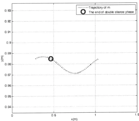
Figure 4-7: The trajectory of the point mass with vo = 2.5465 (m/s) and

p

Figure 4-9: An example of a gait of the springy legged model with double stance phase ... 77

Figure 4-10: Continuity of velocity between the end of a step and the beginning of the next step. . 77 Figure 4-11: Instability of a period-one gait of the springy legged model with double stance ... 80

Figure 4-12: Two initial positions of a springy legged model with double stance phase...82

Figure 5-1: An ankle actuated walking model; definitions of parameters... 86

Figure 5-2: The free body diagram of bar DA in Figure 5-1 ... 87

Figure 5-3: The free body diagram of bar CD in Figure 5-1 ... 87

Figure 5-4: The free body diagram of bar BC in Figure 5-1 ... 88

Figure 5-5: The free body diagram of point mass m in Figure 5-1 ... 89

Figure 5-6: The geometry of the ankle actuated model during double stance phase... 91

Figure 5-7: The sequence of a step of the ankle actuated model; collisions occur at t=to and t=t ... 95

Figure 5-8: Ground reaction force FB of the ankle actuated model with k = 10 (N-m/rad) ... 96

Figure 5-9: Ground reaction force FR of the ankle actuated model with k = 8 (N-m/rad) ... 97

Figure 5-10: 0 and with the selected parameter values and initial speed for the period-one gait. 99 Figure 5-11: Asymptotic stability of the period-one gait of the ankle actuated model... 105

Figure 6-1: The free body diagram of the ankle controlled model in a frontal plane... 110

Figure 6-2: The operating point yielding a straight posture of the ankle-controlled model... 116

Figure 6-3: The fixed point of the ankle controlled model that yields zero torque ... 120

Figure 6-4: The block diagram of the closed loop system of the ankle controlled model... 123

Figure 6-5: Poles of the uncompensated system of the balancing model in a frontal plane... 125

Figure 6-6: Impulsive perturbation acting on B of the ankle controlled model in a frontal plane.. 129

Figure 6-7: Time response of 601 of the model with the input torque in [-10, 10] (N-m)... 129

Figure 6-8: Time response of co1 of the model with the input torque in [-10, 10] (N-m)... 130

Figure 6-9: Time response of 602 of the model with the input torque in [-10, 10] (N-m)... 130

Figure 6-10: Time response of o, of the model with the input torque in [-10, 10] (N-m)... 131

Figure 6-11: The controlled ankle torque of the ankle controlled model in a frontal plane... 132

Figure 6-12: The ground reaction force in the x direction of the ankle controlled model... 132

Figure 6-13: The ground reaction force in the y direction of the ankle controlled model... 133

Figure 6-14: 60, with the perturbation with amplitude of 100, 150, 200 and 250 (N)... 134

Figure 6-15: 5602 with the perturbation with amplitude of 100, 150, 200 and 250 (N)... 135

Figure 6-16: 60, of the ankle controlled model with the perturbation with amplitude of 310 (N).. 135

Figure 6-18: Time response of 6O of the model with the input torque in [-150, 150] (N-m)... 137 Figure 6-19: The free body diagram of a 3-D inverted pendulum hinged at a revolute joint... 138

List of Tables

Table 3-1: The meaning of parameters of a springy legged model without double stance phase ... 44

Table 3-2: Parameter values of the springy legged model without double stance phase... 50

Table 4-1: The meaning of parameters of a springy legged model with double stance phase ... 61

Table 4-2: Parameter and initial state values of the springy legged model with double stance ... 70

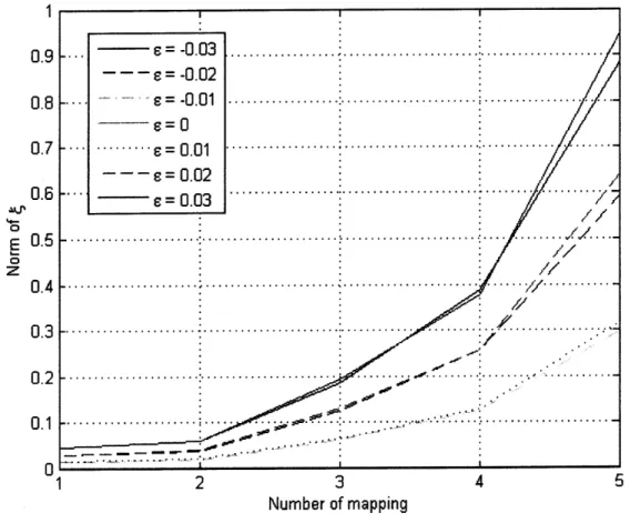
Table 4-3: Eigenvalues of the derivative matrix of Poincare map with varying 6 ... 82

Table 5-1: The meaning of parameters of the ankle actuated model described in Figure 5-1...86

Table 5-2: Selected parameter values for the period-one gait of the ankle actuated model ... 98

Table 6-1: The meaning of parameters of the ankle controlled model in a frontal plane... 110

1. Introduction

1.1.

Motivation and Goals

Some recent developments in rehabilitation techniques in locomotion have turned out to be effective [1]. However, some rehabilitation techniques can be not only effective but also efficient in terms of price or efforts. Efficiency may be achieved by focusing on the recovery of the movement of a specific joint rather than trying to improve the movement of all the joints participating in locomotion. One good starting point is the ankle joint because the ankle is known as the most important actuator in propulsion, in terms of the amount of torque [2]. In this thesis, I establish models actuated or controlled by ankles to provide theoretical fundamentals to assess the effectiveness of rehabilitation therapy focusing on ankles.

Many aspects of bipedal locomotion have been widely studied. Some researchers have analyzed normal gait by solving inverse dynamics [3]. They have measured joint angles and ground reaction forces, so the amount of torque of each joint can be estimated from the measured data. A robot might generate generic human bipedal locomotion by following the command of the

solved torque at each joint. Other researchers have studied human locomotion by designing and testing simple walking machines compared to humans in terms of morphology, gait appearance and energy use [4]. These simple machines fundamentally depend on passive dynamics. Only very simple control is used compared to bipedal walking robots following the solved inverse dynamics of a human gait. The former approach, which uses inverse dynamics, might generate more humanlike or elaborated bipedal walking. In contrast, the latter approach provides more clues to what dynamics bipedal walking involves.

fully studied. Particularly, related to rehabilitation therapy, though some groups have developed therapeutic robots for locomotion by imposing kinematic patterns of leg motion [1], this approach ignores the probable role of dynamics in human locomotion.

The Newman Laboratory for Biomechanics and Human Rehabilitation at the Massachusetts Institute of Technology (MIT) has shown the value of therapeutic robots for upper-extremity rehabilitation [5-9]. Recently, the Newman Laboratory has also developed a two-degree

of freedom therapy robot module for the ankle [10]. My analysis in this thesis can provide a basis

to assess whether and how such a robot module for the ankle may be used for locomotor rehabilitation by investigating the dynamics of a simple model actuated and controlled by ankles.

My study in this thesis consists of two parts-locomotion in a sagittal plane and balancing

in a frontal plane. The main motivation of the analysis of the ankle actuated walking model in a sagittal plane is based on two aspects. On the one hand, experimental data show that ankle torque is larger than knee torque or hip torque during walking [2]. On the other hand, some totally passive walkers can generate stable bipedal gait on a slight slope [11], but they cannot make a stable gait on a horizontal floor. If the ankle torque is the most significant contributor to locomotion not

only in terms of the amount of torque but also in terms of dynamical behavior, one can expect the existence of a stable gait even on a horizontal floor with only ankle actuation.

In particular, I confine my analysis to the existence of a stable period-one gait with actuation of ankles alone. Period-one gaits are the gaits in which a walker recovers its state exactly after one step. There can also be multi-period gaits that show periodicity with the period of two or more steps. In locomotion of animals including humans, these multi-period asymmetric gaits are also common and physically meaningful. However, at this stage, I focus only on the period-one gait that is the most common, basic, and therefore most important mode of normal periodic gait.

Analyzing the contribution of ankle torque in a frontal plane to balancing with one foot or walking is another important problem. One way to assess the role of ankle torque in a frontal plane is to investigate the dynamics of a model controlled by a single joint alone. If a model

whose shape and mechanical properties are similar to those of humans succeeds to balance with one foot using ankle torque control alone, it can support the idea that human balancing in a frontal plane can be achieved with some ankle control and negligible hip control. Accordingly, the success of the model can support rehabilitation strategies focusing on ankle torque in a frontal plane rather than other strategies involving both hip and ankles. With this motivation, I establish a double inverted pendulum model controlled by ankle torque and investigate the controllability and dynamics of the model.

In summary, this study can provide a theoretical basis on which one can develop or improve hardware or algorithms for assistance at the ankle to help recovery of locomotion or balancing after neurological or orthopedic injury. Considering efficiency, rehabilitation therapy focusing on ankles may be less expensive than prior therapies treating all the joints participating in walking or balancing. More basically, apart from efficiency of the therapy, this research can

provide a further understanding of the dynamics of bipedal walking. Particularly, the contribution of ankle actuation to bipedal locomotion in a sagittal plane is evaluated through this study. Additionally, the contribution of ankle torque control to balancing in a frontal plane is studied.

1.2.

Thesis Organization by Chapters

I describe my analysis of the dynamics of passive walkers in a sagittal plane in chapter 2, 3

and 4: analysis of the motion of a rimless wheel is described in chapter 2; analysis of the motion of a springy legged model without double stance phase is described in chapter 3; and, analysis of the

motion of a springy legged model with double stance phase is described in chapter 4.

Subsequently, I present my analysis of the ankle actuated model in chapter 5. With the

understanding of the dynamics of the preceding passive walkers in chapter 2, 3 and 4, I establish a simple model with actuated ankles and analyze the dynamics of the model in a sagittal plane.

In addition, I analyze balancing in a frontal plane with one foot using ankle torque in chapter 6. I make a double inverted pendulum model whose mechanical properties and geometries are similar to those of a human and study the dynamics of the model controlled by one joint representing an ankle.

Finally, I summarize the results and discuss the conclusions and implications in chapter 7. Future directions of the research are also discussed. For readers' information, the source codes that I used and other supplementary contents are attached in the Appendix.

1.3.

Terminology and Notation

Throughout the rest of this thesis, I use the terminology of a stride function and the following notation for expression of vectors, time, evolution rules and discrete maps.

1.3.1. A Stride Function and a Poincare Map

Tad McGeer introduced the stridefunction whose input and output are the state variables such as angles of joints and their derivatives at the beginning of one step and at the beginning of the next step respectively. I extend the concept of the stride function suggested by McGeer by

including leg length and their derivatives in the input and output of the stride function for springy legged models. The motion of a walking model can be expressed as a set of equations of motion,

which usually take the form of differential equations. The solution of the equations can provide a map whose input and output are the state vectors of the beginning of one step and the end of the step respectively. Separated from the set of equations of motion, there is another map whose input and output are the state vectors of the end of one step and the beginning of the following step respectively. The combination of two maps can be considered as a kind of stride function f. In the language of dynamical systems, the stride function can be considered as a discrete Poincard map.

1.3.2. Vector Notation

I use bold print to describe a vector. In addition, without specific definition, i,

j

Sad=axi + ayj + ak = axi + ayj+ a:k .

Eq 1-1

represents the magnitude of the vector that is indicated by the bold print of the character. For

example, a means the magnitude of the vector a. In particular, without specific definitions, the characters with subscript x, y and z indicate the magnitudes of components of the corresponding

vector in positive x, y and z directions respectively. For example, ax =

a

1.3.3. Time Notation

Without specific definition, T_ and T+ represent the time just before and right after time T respectively. T_ and T, are infinitesimally close to time T when an event occurs.

1.3.4. Notation for Maps and Evolution Rules

Without specific definition, italic print such asf; for example, represents an evolution rule of a continuous dynamical system, which might be another expression of a set of equations of motion. Sometimes, italic print such asf; for example, can also represent a simple scalar function. On the other hand, bold print such as f, for example, represents a discrete mapping.

1.4.

Method of Stability Analysis

Stability of the gait of each model is of great importance in this study. As explained in

1.3.1, each step can be considered as a stride function or a Poincard map whose input and output are

some of the state variables at the beginning of one step and the beginning of the following step respectively. A proper set of state variables generating the period-one gait becomes a fixed point

of the stride function. To analyze stability of the period-one gaits, if any, I perform stability analyses by following three steps: (1) I find the fixed points of the Poincare map, if any, which generate the period-one gaits; (2) I analyze the stability by investigating the eigenvalues of the derivative matrix of the Poincard map at the fixed points; and, (3) I visualize the stability or

instability by showing the behavior of the small neighborhood of each fixed point.

1.4.1. Poincare Section and the Reduced State Vector

A Poincard map can be constructed by choosing a proper Poincard section [12]. A

Poincard section is a local cross section in the state space. The dimension of the Poincare section is reduced by one from the original dimension of the state space. A simple visualization is

section, not necessarily aligned with the state space axes. Furthermore, the Poincard section needs not to be planar as long as every flow generated by the evolution rule is transverse to it. In the special cases of my study, I set the Poincard section by simply fixing one state variable for each model as in Figure 1-1.

In this study, the selection of the Poincard section is crucial because the Poincard section acts as an anchor indicating a completion of a step. For example, if I choose the angle between the legs as a state variable fixed at the Poincare section, which indicates the end of one step for a springy legged model, a problem occurs; if the leg length does not recover its initial value at the moment when the angle recovers its initial value, the initial leg length of the following step becomes different from the initial leg length of the preceding step. Then, the energy stored in springy legs can be different at the beginning of each step, which is not desirable.

Hereafter, without specific definition, I define the state vector with reduced dimension that is restricted to the Poincare section as the reduced state vector and express it as a vector with hat.

Please see Figure 1-1. With a Poincard section X, I can define a Poincare map f as f . -+ Z;

ik+1 =f(k), where XEEX.

n dimensional state space, S C R" (xp ,V" x2--Xn) = x E S. n-I dimensional Poincard section, Z with x, = x10 (x21 X1 I... Xn) = x, varies along p A -P= f(P,) this curve. p= f(P,)

Evolution from P. by the CV0lUtion rule of the dynamical system (time grows from 0) Figure 1-1: A schematic explanation of Poincard section

1.4.2. Stability and Asymptotic Stability

Stability and asymptotic stability of a fixed point of a discrete map can be defined as the following:

Definition 1 Let X = Xeq be a fixed point of a discrete map Xk +

f(ik).

V n E N, which is the set of positive integers, 3 5 = 6(e)> 0, such that for V X0,

Xo eq < 6, we have f () 0 -eq < C.

Definition 2 Let X = Xeq be a fixed point of a discrete map Xk +1 = f(ik). The fixed point

X = Xeq is asymptotically stable when X = Xeq is stable and 3 6 = 6(c)> 0 such

that for V jo ,X1 - Ieq < 6, we have I(i)

f

1.4.3. Stability Analysis Using Linearization

Once I consider each step as a Poincard map whose input and output are the reduced state vectors, x 's, at the beginning of one step and the following step respectively, the dynamical system corresponding to each model becomes a discrete dynamical system or a discrete map.

One way to investigate the stability of a fixed point of a map is using linearization, which is conclusive for hyperbolic fixed points [12]. Let X = Xeq +4, where Xeq is a fixed point of a map f, and 4 be a vector indicating a very small error. If (1) the derivative matrix of the map f exists, and (2) the fixed point is hyperbolic, then,

af

f(i)

)

-> f( ) - f (X^eq) af -9

Hence, in cases that (1) and (2) above are met, stability analysis can be performed by investigating

A8ff

eigenvalues of the derivative matrix J( X ) at the fixed point, where J = . If all the eigenvalues

of this derivative matrix are located within a unit circle in a complex plane, the system is asymptotically stable. If there is at least one eigenvalue outside the unit circle, the system is

unstable. If the largest magnitude of the eigenvalues is equal to one, the system is non-hyperbolic and the stability analysis by linearization is no longer conclusive.

In each of the models I analyze, the derivative matrix of the Poincare map exists and the investigated fixed point is hyperbolic. Therefore, stability analysis using linearization is conclusive in the cases of models I analyze in this thesis. A brief proof of the existence of the derivative matrices of the Poincare maps of the analyzed models is derived in Appendix A. The analyses in Chapters 2-5 will help readers to fully understand the proof in Appendix A.

2. A Rimless Wheel Model in a Vertical Plane

To understand the dynamics of a passive walker, I select a rimless spoked wheel model that is constrained in a vertical plane as a starting point. This model is considered as a proper starting point not only because it is simple but also because it captures many of the essential behaviors of bipedal walking. This model imitates foot collision due to foot placement and the inverted-pendulum motion of the single stance phase of bipedal walking. Some prior work has been done analyzing this model in several ways [11, 13].

I analyze the dynamics of the model on a horizontal floor and on a slight slope. I show

that the rimless wheel loses kinetic energy with a constant reduction ratio per collision, and the rimless wheel on a slight slope can make a stable period-one gait with some proper initial condition and selected parameter values.

2.1.

Analysis of the Model on a Horizontal Floor

2.1.1. Assumptions and Definitions of Parameters

A point mass moves in a vertical plane under the influence of gravity, restrained by a rigid

massless leg that rests on the ground but can instantaneously be moved in front of the mass. One way to visualize this model is to imagine a wheel with radial spokes and no rim. The spokes have no mass and wheel has mass but no moment of inertia.

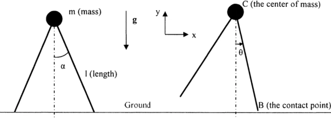
For the definitions of parameters and the coordinate axes, see Figure 2-1. The angle 0 is defined by the orientation of the stance leg.

m (mass)

I (length)

g

Ground

C (the center of mass)

y

x

0

0-B (the contact point)

Figure 2-1: A rimless wheel model on a horizontal floor; a is the initial value of 0

2.1.2. Analysis of Speed of the Point Mass

Let the vector forms of H, M, r, v and P indicate angular momentum, applied torque about a specific point, a position vector from one point to another, a velocity vector and linear momentum respectively.

Figure 2-2 shows the motion of the rimless wheel. The point mass moves as an inverted pendulum, and the leg collides with the ground at point B at time t = to. For the analysis, I divide the dynamic process into two parts: the collision and the phase between collisions.

vvcVt

B i B

t =to. t to,

t <to t> to

Just before a collision Right after a collision

Part 1 - The Collision (to. -+ to,)

The free body diagram (FBD) of the system is shown in Figure 2-3. The impulsive ground reaction force (GRF) is the only contact force. To avoid considering this impulsive force, which is relatively difficult to characterize, I apply the angular momentum principle about point B in Figure 2-3 so that the torque due to the impulsive force is zero. By the angular momentum

principle about B,

H

HB+V1xP = MB= rBcx mg. Eq2-1

Because the velocity of point B is zero, the second term on the left hand side of Eq 2-1 vanishes, and

HB(to+)

(rc

The right hand side of Eq 2-2 equals zero because the time gap between to+ and to- goes to zero, and the integrated term is not impulsive. Therefore, the angular momentum about point B is conserved during the collision, and

HB(to+)

=

HB(to-).

With the assumption that the model finishes its inverted pendulum motion at to and starts a new inverted pendulum motion about B at to+, the velocity vc at t = to can be written

vc(to-) = vo

=

(vo cos a)i

-

(vo sin a)j, and

vc(to+)

=

vi

=

(vi cos a )i + (vi sin a )j,

Eq 2-4

where i and

j

rBC

mvI

HB(to-)

rBc x mvo,

-

(mlvi)k

=

mlvo(sin

_a

-

_cos

_a)k

₌

_{-(mlvo cos 2a)k,}

where k is the unit vector in the direction of +z axis. Finally, by comparing the magnitude of the left hand side and the right hand side of Eq 2-5,

vi= vocos2a.

ng (gravity)

B

F (impulsive GRF)

Figure 2-3: The free body diagram of the rimless wheel at a collision

Part 2 - The Phase between Collisions

The free body diagram (FBD) of the system is shown in Figure 2-4. By the assumption

of massless legs, force F, which is the ground reaction force (GRF), must be directed toward point

C in Figure 2-4. In other words, force F is always parallel with the position vector rBc. The consequence of the parallel direction of F with rc is this: when I analyze the motion of the inverted pendulum by decomposing it into the tangential and normal directions, there is no contact force applied in the tangential direction. Hereafter, I refer to this fact as @. Also, force F does no

work during the inverted pendulum motion because point B, as shown in Figure 2-4, does not move.

I refer to this fact as ®. I will depend on facts @ and 0 to find the critical values of the initial speed.

C

rng

B

F (GRF)

Figure 2-4: The free body diagram of the rimless wheel between collisions

Minimum Speed for the System to Make the Next Step

I investigate the critical speed VICr or VOCr that makes the velocity zero at the apex (0 = 0)

after the collision. If the initial speed is less than this critical value, the rimless wheel cannot vault

over and cannot make the next step.

Because of 0, the only working force applied to the system is gravity, which is a conservative force. Therefore, the total mechanical energy of the system is conserved between

collisions. If v1 = vicr, the total mechanical energy becomes -mvicr 2 + 0 = 0 + mgl(1 - cosa), 2

and vicr is obtained as

VICr = 2gl(1 - cos a) . Eq 2-7

V 2gl(1

cosa)

VOCr = _E

-cos 2a

Maximum Speed for the System Not to Leave the Floor

With the assumption that the model starts a new inverted pendulum motion about point B in Figure 2-4, 1 establish the equation of motion in the normal and the tangential components; see Figure 2-5. For any motion, the acceleration can be decomposed into two components: one is the tangential component, and the other is the normal component. If I define the radius of curvature as p, then,

d

dv

v

-dV

et +

en.

Hence, the equation of motion of the rimless wheel becomes

d -

dv -

v2

-m iV

= m

e,+m

= mg +

F

= mg cos

Oen

- mg sin

Oet

- Fen

_{Eq 2-10}

= -mg sin Qet + (mg cos 0 - F)en.

et C

en p

x

To investigate the maximum speed for the system not to leave the floor, I confine my interest to the normal component only. Extracting the normal components from Eq 2-10,

m

= Mg Cos

0

- F

->

F = mg cos

0 - M

f

Let the right hand side of Eq 2-11 bef(0). Physically, leaving the floor indicates zero magnitude of F (GRF) in Figure 2-4. Hence, to keep the model attached on the floor, I must keep the minimum off(O) above zero.

By conservation of mechanical energy during the inverted pendulum motion, the kinetic

energy reaches the maximum when the point mass is at the lowest position in y. Therefore, v2 reaches the maximum when 0 = -a or +a. Also, cosO becomes the minimum when 0 = -a or +a (-E/2<- a <0 < a <7c/2). As a result,f(0) becomes the minimum when 0 = -a or + a, and I need

v12

(cos

_2a)vo

min(F)= mg cosa -m

2 = mg cosa -im

>0, or

)glcosa

VO co .a Eq 2-12

cos2a

Considering that the speed is reduced by the factor of cos2a due to the collision, it is more meaningful to find the maximum initial speed in pure x direction that keeps the wheel from flying off. The maximum initial speed can be obtained by the same procedure, resulting in

Qgicosa

gi

VO -= . Eq 2-13

cos a

cos a

2.1.3. Further Analysis

The Range of a

Eq 2-8 implies that if a =7c/4, the model can never vault over regardless of the initial speed.

opposite to the direction of the momentum. Therefore, the point mass cannot use its momentum to vault over; see Figure 2-6.

a =/4

B F

Figure 2-6: The rimless wheel model with a =7r/4

If a > n/4, Eq 2-8 yields a meaningless result, indicating that there exists some negative

speed that can make the model vault over. By confining the range of a to (0, n/4), which is also reasonable for human bipedal walking, I can preclude such misleading solutions.

From Eq 2-8 and Eq 2-12, it is suggested that the initial speed vo must satisfy 2g1(1 -cos a) gl coscc

< Vo < for the model to generate a reasonable gait. This

cos2a cos2a

inequality has meaning only when 2g(l -cos a) < gl cos a , or cos a > 2 /3, which means

O<a<0.84. This range includes (0, n/4). Therefore, I can confine my interest to the case of a E (0, a/4).

Mechanical Energy Loss per Step

Eq 2-6 implies that the kinetic energy of the system, which is proportional to v2

, is reduced by a factor of cos2_{2a per collision.}

increases. In contrast, mechanical energy is conserved during the inverted pendulum motion. Consequently, the energy is lost per step, and there is no way to compensate for the lost energy. Therefore, any periodic gaits cannot be observed in this model. After finite steps, the rimless wheel on a horizontal floor cannot vault over, and it fails to make the next step.

2.2.

Analysis of the Model on a Slight Slope

2.2.1. Assumptions and Definitions of Parameters

A point mass moves in a vertical plane under the influence of gravity, restrained by a rigid

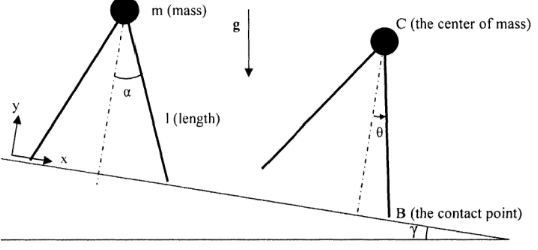
massless leg that rests on the ground but can instantaneously be moved in front of the mass. The model is placed on a slight slope so that gravity can do work on each step. For the definitions of parameters and the coordinate axes, see Figure 2-7. I assume that a is greater than y. The angle 0 is defined by the orientation of the stance leg.

m (mass)

g C (the center of mass)

a

I (length)

'grB (the contact point)

2.2.2. Analysis of Speed of the Point Mass

The meaning of H, M, r, v and P is consistent with the meaning of H, M, r, v and P in 2.1.2. See Figure 2-7. The point mass moves as an inverted pendulum, and the leg collides with the ground at point B at time t = to. For the analysis, I divide the dynamic process into two parts: the collision and the phase between collisions.

Part 1 - The Collision (to. -+ to,)

By the same procedure as in 2.1.2,

HB(to+) = HB(to-). Eq 2-14

In other words, the angular momentum about point B in Figure 2-7 is conserved during the collision. With the assumption that the model finishes its inverted pendulum motion at to-and starts a new inverted pendulum motion about point B in Figure 2-7 at to+, the velocity vc at t = to can be written

vC(to-) = vo = (vo cos a)i - (vo sin a)j, and

vc(to+) = vi = (vi cos a)i + (vi sin a)j, Eq 2-15

where i and

j

Eq 2-15,

rBC X mvI =

HB(to+)

-(mlvi)k = mlvo(sin2 _{a - cos}2 _{a)k = -(mlvo cos 2a)k ,}

Eq 2-16

where k is the unit vector directed along the +z axis. Finally, by comparing the magnitude of the left hand side and the right hand side of Eq 2-16,

vi = vo cos 2a. Eq 2-17

This is the same result as Eq 2-6 of 2.1.2 .

Part 2 - The Phase between Collisions

The free body diagram (FBD) of the system is shown in Figure 2-8. Note that gravity applies in an oblique direction because the x axis in Figure 2-8 is parallel with the surface of the slope. As mentioned in 2.1.2, F (GRF) must be directed toward C all the time. In other words, force F is always parallel with the position vector rBC. Also, point B does not move during the phase between collisions. Therefore, @ and

®

C y 0 x mg B F (GRF)

Figure 2-8: The free body diagram of the rimless wheel on a slope between collisions

Minimum Speed for the System to Make the Next Step

I investigate the critical speed viCr or vocr that makes the velocity zero at the apex (0 0)

after the collision. If the initial speed is less than this critical value, the rimless wheel cannot vault

gravity, which is a conservative force. Therefore, the total mechanical energy of the system is conserved between collisions.

If vI = vIcr, the total mechanical energy becomes -mvIr 2

+ 0 = 0 + mg{1 - cos(a - y)}

2

and vicr is obtained as

VICr = 2g{1 - cos(a - y)} . Eq 2-18

In terms of vo, the minimum speed that makes the model vault over is

2g{1

cos(a

y)}

VOCr = Eq 2-19

cos 2a

Maximum Speed for the System Not to Leave the Floor

I establish the equation of motion in the normal and the tangential components. The equation of motion becomes

d - dv v 2 -m d V=M e+mFen

= mk

mg cos(O - y)en

=

To investigate the maximum speed for the system not to leave the floor, I confine my interest to the normal component only. Extracting the normal components from Eq 2-20,

m V mg cos(O - y) - F -> F = mg cos( - y ) -m V2 = h( ). Eq 2-21

As explained in 2.1.2, to keep the model attached on the floor, I need to keep the minimum of h(O) above zero.

By conservation of mechanical energy during the inverted pendulum motion between two

potential energy becomes its minimum. Therefore, v2

reaches the maximum when 0 = -a. Also, assuming that 0 <a <7c/2 and 0 < y <a, cos(0 - y) becomes the minimum when 0 = -a. As a result,

h(0) becomes the minimum when 0 = -a, and I need

M2

min(F)= mgcos(a

+

)

-

m

/

>0.

Because of @ in 2.1.2, I can apply conservation of mechanical energy to find v2

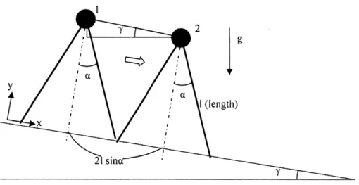
when 0 = -a. Figure 2-9 shows that the work done by gravity per step can be written

WI

2=mgor]2=

2mgl sin

a

sin y

Then, from A-mv2 ₌

2mgsinasiny, Eq 2-22 and Eq 2-23,

2

-I

(cos22a)vo

+4glsinasiny 0. Eq 2-24

=mgcos(ay)-m.2

jgl{ cos(a +y) -4 sin a siny}

cos2a

The maximum speed in the pure x direction that keeps the wheel from flying off can be obtained by the same procedures, resulting in

vo

,

gl{cos(a +,y) - 4 sin a siny}

cos a

2 2

g

I (length)

x

21 sina'

Figure 2-9: The rimless wheel on a slope at the begning and at the ending of a step

The Range of a

From Eq 2-19 and Eq 2-25, it is suggested that the initial speed vo must satisfy

V2gl{l - cos(a - )/)} < v< gcos(a + y) - 4 sin a sin y}g~

cos 2a cos 2a

This inequality has meaning only when 2gl{1 - -cos(a - y)} < Vgljcos(a + y) - 4 sin a sin y}) or 0 <2 - 2cos(a - y) <cos(a +y) - 4sin asin y. I confine my interest to the range of a in which a

satisfies this inequality.

2.2.3. Existence of a Period-One Gait

The kinetic energy of the system, which is proportional to V2, is reduced by the factor of

cos2_{2ca per collision. However, it regains some kinetic energy during the inverted pendulum} motion because gravity does non-zero work per step. Therefore, the kinetic energy may either increase or decrease throughout one step. Furthermore, it is possible that there exists a critical

case in which the kinetic energy at the end of one step is same as the kinetic energy at the end of the next step. The work done by gravity is obtained from Eq 2-23. To compensate for the loss of kinetic energy due to collision by the work done by gravity, I need

1

2mgl sin a sin y

-mvo2 (1 cos

_{a), or}

2

2

4glsinasiny

1-cos

_2a

Therefore, some elaborately tuned initial velocity can make a period-one gait.

Each step can be considered as a stride function or a Poincard map, and the state vector generating the period-one gait becomes a fixed point of the stride function. In this case, there exists a unique fixed point. One important issue is the stability of the fixed point. In the following sections, I investigate the stability of the fixed point in a qualitative and quantitative way.

2.2.4. Stability Analysis of the Period-One Gait

Qualitative Analysis

The period-one gait of the rimless wheel is expected to be stable. With enough but not excessive initial speed vo, which is suggested in 2.2.2, the system obtains either increased or decreased speed at the end of an inverted pendulum motion; see Figure 2-9. Let KEl be the kinetic energy at position I (just before the collision), and KE2 be the kinetic energy at position 2 (just before the collision). Suppose that KEl is larger than the kinetic energy of the period-one gait at the same moment. Then, at the following collision, the system suffers greater loss than the case of the period-one gait because the reduction ratio is always cos2

2a. Then, it becomes impossible for the work done by gravity to compensate for the loss of kinetic energy. Therefore,

KE2 becomes smaller than KEl. After repeating such progress for several steps, KE(n) becomes small enough that work done by gravity can compensate for the loss of kinetic energy. Then, the kinetic energy settles down at the kinetic energy of the period-one gait. Similar argument applies to the case in which KEl is smaller than the initial kinetic energy of the period-one gait.

However, the asymptotic stability of the fixed point can be observed only when this system is guaranteed to vault over and not to fly off the slope at every step. In other words, at every collision, the speed just before the collision must be between the maximum and minimum speeds discussed in 2.2.2. For example, if the initial speed is so small that the system fails to vault over, it cannot show the stable period-one gait.

Quantitative Analysis

As mentioned in 1.4, I treat the stride function of each step as a Poincard map and analyze the stability of the fixed point of the map. To construct the Poincard map, I need to obtain the equation of motion of the system and express the dynamical system in state space representation. After constructing Poincard map, I perform stability analysis by following three steps: (1) 1 find the

fixed point of the Poincare map that generates the period-one gait, which is already done in 2.2.3; (2) I confirm the asymptotic stability by investigating the eigenvalues of the derivative matrix of the Poincare map at the fixed point; and, (3) I visualize the asymptotic stability by showing the behavior of the small neighborhood of the fixed point.

Equation of Motion

Please consult Figure 2-7 and Figure 2-8. As explained in 2.2.2, the speed reduces by the factor of cos2a during the collision. For the phase between collisions I can derive equations of motion using the Lagrangian approach. Note that the only constraint force is the ground reaction

force (GRF) that does no work by the assumption of fixed B. Therefore, the constraint is ideal. Also, the active force, gravity, is a conservative force. As a result, all non-potential generalized forces are zero.

Let L, T and V be the Lagrangian, kinetic energy and potential energy respectively.

L =T -V =--m(l) 2 _{-mglcos(O --y), and}

2

d L =0 sin(- y)=0. _Eq2-28

dt aO a(

1

Eq 2-28 is the equation of motion during the phase between collisions

Poincar6 Section

Please see Figure 2-7. The angle 0 is a generalized coordinate of this dynamical system. From Eq 2-28, the equation of motion is expressed in a second-order ordinary differential equation, and I need two state variables 0 and dO/dt to describe this dynamical system in state space. For this system, a completion of one step can be indicated by the value of 0; a step is regarded as completed when 0 goes from a to -a. In other words, a proper Poincard section is anchored at the sub-state space where 0 becomes ± a. In conclusion, the Poincard map corresponding to the stride function of this model is defined in the one dimensional Poincard section E, which is

Z ={(0,)= ±a and Oe R}.

Fixed Points of a Poincar6 Map

As mentioned in 2.2.3, there is a unique fixed point of the rimless wheel on a slope with

the initial speed of vo = 4gl sin a sin ' . This initial speed makes constant kinetic energy at 1- cos 22a

every moment just before a collision, and the fixed point of the Poincare map can be directly obtained from this initial speed.

Stability Analysis Using the Derivative Matrix of the Poincare Map

I prove the existence of the derivative matrix of the the Poincard map in Appendix A. 1.

Then, rigorous proof of asymptotic stability can be achieved by showing that all the eigenvalues of the derivative matrix of the Poincard map stay inside a unit circle. With the selected Poincar6 section, I construct the Poincard map and its derivative matrix both analytically and numerically. Then, I investigate the eigenvalues of the derivative matrix at the fixed point both analytically and numerically.

With the definitions of X = = and = (x2) =(),the numerical construction

of the Poincard map is performed as the following:

Step 1 Solve the obtained equation of motion (Eq 2-28) with a given initial condition. Step 2 Find the minimal positive time when 0 becomes -a, and define the time as Tf. Tf

is the time when the collision occurs. Step 4

Step 5

Find the reduced state vector X= (x 2) = (dO/dt) at Tf_, which is the time just

before the collision

Find the reduced state vector X= (x2) = (dO/dt) at Tf+, which is the time right

after the collision. _{Using the result of analysis of the collision in 2.2.2,}

y.= = (cos 2a)

y.-As a result, the Poincare map, f is summarized schematically as the following:

X2

f(x)

sin(xi

,and

() = =T.+

(cos2a)i

(cos2a))

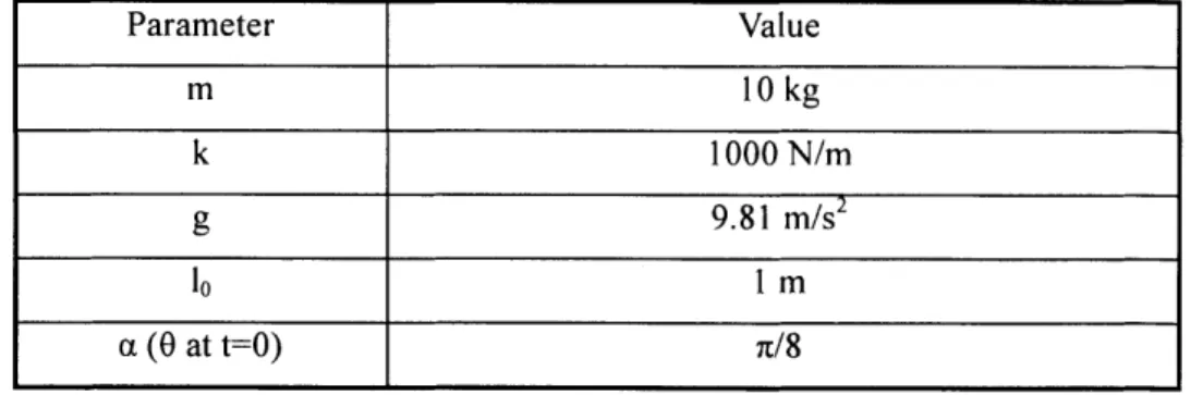
tTf-Once I construct the Poincard map, I can also construct the derivative matrix of the Poincard map. In this case, the only varying state variable is the initial angular speed, dO/dt, so the reduced state vector X and the derivative matrix become a scalar and a one-by-one matrix respectively. With parameter values of m = 10 (kg), g = 9.81 (m/s2

), 1 = 1 (M), a = 22.5 (deg)

(n/8 rad) and y = 5.73 (deg) (0.1n rad), the eigenvalue of the derivative matrix of the Poincard map

at the fixed point is found to be 0.5, which is located inside the unit circle. This guarantees the asymptotic stability of the fixed point of the map.

On the other hand, I can also construct the Poincard map analytically using a work-energy principle. Using a work-energy principle and following the argument in Appendix A.1, the Poincard map becomes

cos 2a

I m

the derivative matrix of the map becomes

Of (io) 0+..

N

axo -2 4mg/sin asin y

M12

The fixed point of the Poincard map can be obtained from energy balance or from Eq 2-27. Considering Eq 2-27 solves the speed just before the collision when the system is at the fixed point,

O(t

O(t

I I-cos2

derivative matrix of the Poincard map at the fixed point becomes

af(io)

-cos2a

₊

= cos

2a.

aio

sin a sin y

M12do,=- cosa 4g/sinasiny I V -cos 2 2a

With parameter value of a = 22.5 (deg) (n/8 rad), the eigenvalue of the derivative matrix of the Poincard map at the fixed point is obtained analytically to be 0.5, which is the same result of the numerical work.

Both Analytical and numerical analysis guarantees the asymptotic stability of the fixed point. However, it is important to note that as explained already, the asymptotically stable fixed point can be observed only when this system is guaranteed to vault over and not to fly off the slope at every step. In other words, at every collision, the speed just before the collision must be between the maximum and minimum speeds discussed in 2.2.2.

Visualization of Asymptotic Stability

I first check if the analytically obtained fixed point behaves like a fixed point of the

Poincard map that is numerically constructed. Then, I investigate the behavior of the small neighborhood of this fixed point. Please consult Figure 2-7. With parameter values of m = 10

(kg), g = 9.81 (m/s2

), 1 = 1 (m), a = 22.5 (deg) (7/8 rad) and y = 5.73 (deg) (0.12I rad), the speed just before a collision when the system is at the fixed point is obtained as 1.73 (m/s) from Eq 2-27. The corresponding angular speed is 1.73 (rad/s) and angular speed of investigated neighborhood varies from 1.43 (rad/s) to 2.03 (rad/s). This investigated neighborhood is totally included in the speed range whose upper limit and lower limit are the marginal value for the system to fly off and vault over respectively. Asymptotic stability is found in this small neighborhood as Figure 2-10 shows.