HAL Id: hal-01320010
https://hal.archives-ouvertes.fr/hal-01320010
Submitted on 20 Sep 2016
HAL is a multi-disciplinary open access
archive for the deposit and dissemination of
sci-entific research documents, whether they are
pub-lished or not. The documents may come from
teaching and research institutions in France or
abroad, or from public or private research centers.
L’archive ouverte pluridisciplinaire HAL, est
destinée au dépôt et à la diffusion de documents
scientifiques de niveau recherche, publiés ou non,
émanant des établissements d’enseignement et de
recherche français ou étrangers, des laboratoires
publics ou privés.
On the usability of deep networks for object-based
image analysis
Nicolas Audebert, Bertrand Le Saux, Sébastien Lefèvre
To cite this version:
Nicolas Audebert, Bertrand Le Saux, Sébastien Lefèvre. On the usability of deep networks for
object-based image analysis. International Conference on Geographic Object-Based Image Analysis
(GEO-BIA), Sep 2016, Enschede, Netherlands. �hal-01320010�
ON THE USABILITY OF DEEP NETWORKS FOR OBJECT-BASED IMAGE ANALYSIS
Nicolas Audeberta, b, Bertrand Le Sauxa, Sébastien Lefèvreb
a
ONERA, The French Aerospace Lab, F-91761 Palaiseau, France (nicolas.audebert,bertrand.le_saux)@onera.fr
b
Univ. Bretagne-Sud, UMR 6074, IRISA, F-56000 Vannes, France - [email protected]
KEY WORDS: deep learning, vehicle detection, semantic segmentation, object classification
ABSTRACT:
As computer vision before, remote sensing has been radically changed by the introduction of Convolution Neural Networks. Land cover use, object detection and scene understanding in aerial images rely more and more on deep learning to achieve new state-of-the-art results. Recent architectures such as Fully Convolutional Networks (Long et al., 2015) can even produce pixel level annotations for semantic mapping. In this work, we show how to use such deep networks to detect, segment and classify different varieties of wheeled vehicles in aerial images from the ISPRS Potsdam dataset. This allows us to tackle object detection and classification on a complex dataset made up of visually similar classes, and to demonstrate the relevance of such a subclass modeling approach. Especially, we want to show that deep learning is also suitable for object-oriented analysis of Earth Observation data. First, we train a FCN variant on the ISPRS Potsdam dataset and show how the learnt semantic maps can be used to extract precise segmentation of vehicles, which allow us studying the repartition of vehicles in the city. Second, we train a CNN to perform vehicle classification on the VEDAI (Razakarivony and Jurie, 2016) dataset, and transfer its knowledge to classify candidate segmented vehicles on the Potsdam dataset.
1. INTRODUCTION
Deep learning for computer vision grows more popular every year, especially thanks to Convolutional Neural Networks (CNN) that are able to learn powerful and expressive descriptors from images for a large range of tasks: classification, segmentation, de-tection . . . This ubiquity of CNN in computer vision is now start-ing to affect remote sensstart-ing as well, as they can tackle many tasks such as land use classification or object detection in aerial images. Moreover, new architectures have appeared, derived from Fully Convolutional Networks (Long et al., 2015), able to output dense pixel-wise annotations and thus able to achieve fine-grained clas-sification. Such architectures have quickly become state-of-the-art for popular datasets such as PASCAL VOC2012 (Everingham et al., 2014) and Microsoft COCO (Lin et al., 2014). In an Earth Observation context, these FCN models are now especially ap-pealing, as dense prediction allows us performing semantic map-ping without requiring any pre-processing tricks. Therefore, us-ing FCN for Earth Observation means we can shift from super-pixel segmentation and region-based classification (Lagrange et al., 2015, Audebert et al., 2016, Nogueira et al., 2016) to fully supervised semantic segmentation (Marmanis et al., 2016).
FCN models have been successfully applied for remote sensing data analysis, notably land cover mapping on urban areas (Mar-manis et al., 2016, Paisitkriangkrai et al., 2015). For example, FCN-based models are now the state-of-the-art on the ISPRS Vaihingen Semantic Labeling dataset (Rottensteiner et al., 2012, Cramer, 2010). Therefore, even though remote sensing images do not share the same structure as natural images, traditional com-puter vision deep networks are able to successfully extract seman-tics from them, which was already known for deep CNN-based classifiers (Penatti et al., 2015). This encourages us to investigate further: can we use deep networks to tackle an especially hard re-mote sensing task, namely object segmentation ? Therefore, this work focuses on using deep convolutional models for segmenta-tion and classificasegmenta-tion of vehicles using optical remote sensing data.
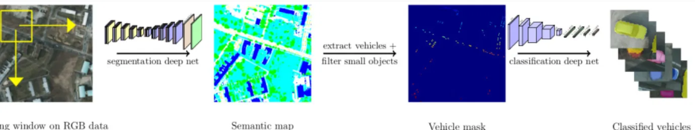
To tackle this problem, we design a two-step pipeline for segmen-tation and classification of vehicles in aerial images. First, we use
the SegNet architecture (Badrinarayanan et al., 2015) for seman-tic segmentation on the ISPRS Potsdam dataset. This allows us generating a pixel-level mask on which we can extract connected components to detect the vehicle instances. Then, using a CNN trained on vehicle classification using the VEDAI dataset (Raza-karivony and Jurie, 2016), we classify each instance to infer the vehicle type and to eliminate false positives. We then show how to exploit this information to provide new pieces of data about vehicle types and vehicle repartition in the scene.
Our work is closesly related to (Marmanis et al., 2016, Paisitkri-angkrai et al., 2015) who also use Fully Convolutional Network for urban area mapping. However we focus only on small ob-jects, namely vehicles, although we use the full semantic map-ping as an intermediate product in our pipeline. Moreover, re-garding (Paisitkriangkrai et al., 2015), our work rely solely on the deeply learnt representation of the optical data, as we do not include any expert features in the process. On the vehicle detec-tion task, (Chen et al., 2014) tried to detect vehicle in satellite images using deep CNN, but only regressed the bounding boxes. On the contrary, our pipeline is able to infer the precise object segmentation, which could be regressed into a bounding box if needed. In addition, we also classify the vehicles into several subcategories using a classifier trained on a more generic dataset, thus performing transfer learning.
2. PROPOSED METHOD
2.1 Semantic segmentation
Many deep network architectures are available for semantic seg-mentation, including the original FCN (Long et al., 2015) or many variants such as DeepLab (Liang-Chieh et al., 2015). We choose to use the SegNet architecture (Badrinarayanan et al., 2015), since it is well-balanced between accuracy and computational cost. Seg-Net’s symmetrical structure and its use of pooling/unpooling lay-ers is very effective for precise relocalisation of features accord-ing to its authors. Indeed, preliminary tests underlined that Seg-Net performs very well, including for small object localization. Results with other architectures such as FCN reported either no
Figure 1. Illustration of our vehicle segmentation + classification pipeline
improvement or an unsignificant improvement. However, note that any deep network trained for semantic segmentation can be used in our pipeline.
SegNet is based on the convolutional layers of the VGG-16 model (Simonyan and Zisserman, 2014). VGG-16 was designed for the ILSRVC competition and trained on the ImageNet dataset (Rus-sakovsky et al., 2015). Each block of the encoder is comprised of 2 or 3 convolutional layers followed by batch normalization (Ioffe and Szegedy, 2015) and rectified linear units. A maxpooling layer reduces the dimensions between each block. In the decoder, sy-metrical operations are applied in the reverse order. The unpool-ing operation replaces the poolunpool-ing in the decoder: it relocates the value of the activations into the mask of the maximum values (“argmax”) computed at the pooling stage. Such an upsampling results in a sparse activation map that is densified by the con-secutive decoding convolutions. This allows us upsampling the feature activations up to the original input size, so that after the decoder, the final output feature maps have the same dimensions as the input, which is necessary for pixel-level inference.
We initialize the weights of the encoder using VGG-16’s weights trained on ImageNet. By doing so, we leverage the expressive-ness of the filters learned by VGG-16 when training on this very diverse dataset. This initialization allows us improving the final segmentation accuracy compared to a random initialization and also makes the model converge faster.
We train SegNet on semantic segmentation on the ISPRS Pots-dam dataset. This translates to pixel-wise classification, i.e each pixel is classified as belonging to one class from the ISPRS bench-mark: “impervious surface”, “building”, “tree”, “low vegetation”, “car” or “clutter”. From this semantic map, we can then extract the vehicle mask which labels all the pixels inferred to belong to the “car” class.
2.2 CNN classification
After generating the full semantic map from one tile, we can tract the vehicle mask. We perform connected components ex-traction to find all candidate vehicles in the predicted map. To separate vehicles that are very close to each other in the RGB im-age and that might belong to the same connected component, we use a morphological opening to open the gap and separate the ob-jects. In addition, to smooth the predictions and eliminate small artifacts and imperfections from SegNet’s predicted map, we re-moved connected components that are too small to be a vehicle (surface < 32 px). For each vehicle (any remaining connected component), we extract a rectangular patch around its bounding box, including 16 px of spatial context on all sides. This patch is then fed to a CNN classifier trained to infer the vehicle’s precise class. The full pipeline is illustrated in Figure 1.
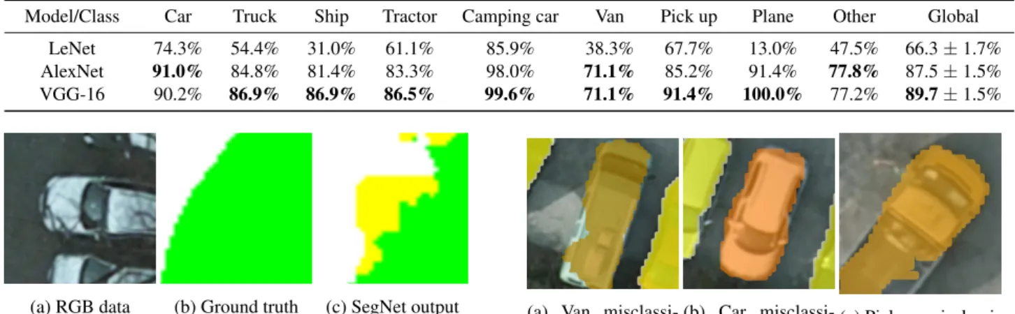
We compare 3 CNN for vehicle classification: LeNet (Lecun et al., 1998), AlexNet (Krizhevsky et al., 2012) and VGG-16 (Si-monyan and Zisserman, 2014). We use the VEDAI dataset to
train these models, so that the Potsdam vehicles will be entirely unseen data. This is to show how knowledge learnt by deep net-works on remote sensing data can be transferred efficiently from one dataset to another, under the assumption that provided reso-lutions (12.5cm) and data sources (RGB) are the same. The clas-sifiers learn to discriminate between the following 11 classes of vehicles from VEDAI, with a very high variability: “car”, “camp-ing car”, “tractor”, “truck”, “bike”, “van”, “bus”, “ship”, “plane”, “pick up” and “other vehicles”.
LeNet is a model introduced by (Lecun et al., 1998) designed for character recognition in greyscale image. Our version takes in input a 224 × 224 color image. It is a comparatively small model with few parameters (' 461K parameters) that can be trained very quickly.
AlexNet is a very popular model introduced in (Krizhevsky et al., 2012) that won the ILSVRC challenge in 2012. It takes in input a 227 × 227 color image. As there are three final fully connected layers, AlexNet is a relatively big network with 61M parameters. We fine-tune the last layer of the reference ImageNet trained implementation of AlexNet.
Finally, VGG-16 is another popular model designed by (Simonyan and Zisserman, 2014), on which is based the SegNet segmenta-tion network introduced in Secsegmenta-tion 2.1. It outperformed AlexNet on the ImageNet benchmark in 2014. It takes in input a 224×224 color image. VGG-16 is the biggest of our three models with 138M parameters. Once again, we fine-tune only the last layer of the reference weights of VGG-16 trained on ImageNet. It is the biggest and slowest of the three models tested in this work.
3. EXPERIMENTS
3.1 Experimental setup
3.1.1 VEDAI This VEDAI dataset (Razakarivony and Jurie, 2016) is comprised of 1268 RGB tiles (1024 × 1024px) and the associated IR image at 12.5cm spatial resolution. For each tile, annotations are provided detailing the position of the vehicles and the associated bounding box (defined by its 4 corners). We cross-validated the results on three of the suggested splits of the dataset for the training and testing sets. The training set for the CNN is built by extracting square patches around each vehicle bounding box, padded with 16 px of spatial context on each side. We use data augmentation to increase the number of samples by includ-ing rotated (π2, π and 3π2 ) and mirrored versions of the patches containing vehicles.
We train each model during 50 epochs (' 1000000 iterations) with a batch size of respectively 128 for LeNet and AlexNet and 32 for VGG-16, and a learning rate of 0.001, divided by 10 after 30 epochs. Training takes about 25 minutes for LeNet, 60 min-utes for AlexNet and 10 hours for VGG-16 on NVIDIA K20c GPU.
Table 1. Average CNN accuracies on VEDAI (3 train/test splits)
Model/Class Car Truck Ship Tractor Camping car Van Pick up Plane Other Global LeNet 74.3% 54.4% 31.0% 61.1% 85.9% 38.3% 67.7% 13.0% 47.5% 66.3 ± 1.7% AlexNet 91.0% 84.8% 81.4% 83.3% 98.0% 71.1% 85.2% 91.4% 77.8% 87.5 ± 1.5% VGG-16 90.2% 86.9% 86.9% 86.5% 99.6% 71.1% 91.4% 100.0% 77.2% 89.7 ± 1.5%
(a) RGB data (b) Ground truth (c) SegNet output
Figure 2. Car partially occluded by a tree on the Potsdam dataset and misclassification according to the ground truth
3.1.2 ISPRS Potsdam This ISPRS Potsdam Semantic Label-ing dataset (Rottensteiner et al., 2012) is comprised of 38 RGB tiles (6000 × 6000 px) and the associated IR and DSM images at 5cm spatial resolution. A comprehensive ground truth is provided for 24 tiles, which are the tiles we will work with. We split ran-domly the dataset in train/validation/test with 70/10/20 propor-tions. For a fair comparison of the two datasets (ISPRS Potsdam and VEDAI) in the same framework, we only use the RGB data and downsample the resolution from 5 cm/pixel to 12.5 cm/pixel. However, note that SegNet would perform even better for small object segmentation on the high resolution tile.
We build our segmentation training set by sliding a window of 128 × 128 px over each high resolution tile, including an over-lap of 75% (32 px stride). For this experiment, we use all the classes from the ground truth. This means that we not only train the model to predict the vehicle mask, but also to assign a label to each pixel according to the ISPRS classes, except “clutter”: “impervious surface”, “building”, “tree”, “low vegetation” and “car”. The model is trained by Stochastic Gradient Descent for 10 epochs (' 100000 iterations) with a batch size of 10 and a learning rate of 0.1, divided by 10 after 3 and 8 epochs. This takes around 24 hours with a NVIDIA K20c GPU.
At testing time, we process the tiles by sliding a window of 128× 128 px with an overlap of 50%. For overlapping pixels, we av-erage the multiple predictions on each pixel. Processing one tile takes around 70 seconds on a NVIDIA K20c GPU. The predicted semantic map contains all classes from the ISPRS benchmark. We extract only the mask for the “car” class as we are mainly in-terested in how SegNet behaves for small objects, especially vehi-cles. We report results before and after removing objects smaller than a predefined threshold.
To compute vehicle classification metrics, we build manually an enhanced ground truth by subdividing the “car” class into several subcategories: “cars”, “vans”, “trucks”, and “pick ups”. We dis-card other vehicles that are present in the RGB data (especially construction vehicles) but not in the original ground truth.
3.2 Results
3.2.1 VEDAI As detailed in Table 1, both VGG-16 and AlexNet are able to discriminate between the different classes of the VEDAI dataset, with respectively 89.7% and 87.5% global accuracy. LeNet is lagging behind and performs significantly worse than its deeper counterpart, with an accuracy of only 66.3%. This result is not
(a) Van misclassi-fied as truck
(b) Car misclassi-fied as van
(c) Pick up misclassi-fied as van
Figure 3. Successful segmentation but misclassified vehicles in the Potsdam dataset
surprising, as LeNet is a very small network in comparison to both AlexNet and VGG-16 and therefore has a dramatically lower expressive power. The LeNet model performs adequately on “easy” classes, such as cars and camping cars, that have low intra-class variability and high inter-class variability. However, it does not work well on vans, which are difficult to distinguish from cars from bird’s view. Moreover, classes with high intra-class vari-ability (especially trucks and planes) are often misclassified by LeNet.
Indeed, we argue that as VGG-16 and AlexNet were pre-trained on ImageNet and fine-tuned on VEDAI, these models were al-ready initialized with very powerful and expressive visual de-scriptors learnt on a highly diverse image dataset. Therefore, both networks benefited from a pre-training phase on a compre-hensive dataset of natural images requiring complex filters able to analyze shapes, textures and colors, which helped training on VEDAI, even though ImageNet does not contain any remote sens-ing image. This fine-grained recognition based on textures and shape allow the CNN to discrminate between classes with a low inter-class variability such as cars and vans, and perform well on classes with high intra-class variability such as planes or trucks. This supports evidence that transfer learning and fine-tuning of ImageNet-trained deep convolutional neural networks is an ef-fective way to process aerial images as shown in previous works (Penatti et al., 2015).
3.2.2 ISPRS Potsdam
Vehicle segmentation The overall accuracy of the SegNet se-mantic mapping on the downsampled ISPRS dataset is 89.5%, excluding clutter and eroding borders by 3 px. Compared to the state-of-the-art result of 90.3%1, this result is quite good consid-ering that we use a downscaled version of the data2. When con-sidering only the “car” class (which comprises all kinds of ter-restrial motorized vehicles), the F1 score at pixel level is 88.4% (95.5% with the eroded borders). We also report a pixel-wise precision of 87.8% and a recall of 89.0%. This indicates that the vehicle mask generated from SegNet’s semantic map should be very accurate and can be used for further object-based analysis.
1http://www2.isprs.org/potsdam-2d-semantic-labeling.
html
2However, we only report our result on a validation set and not on the
full testing set, as full semantic mapping of the ISPRS Potsdam dataset is out of the scope of this work.
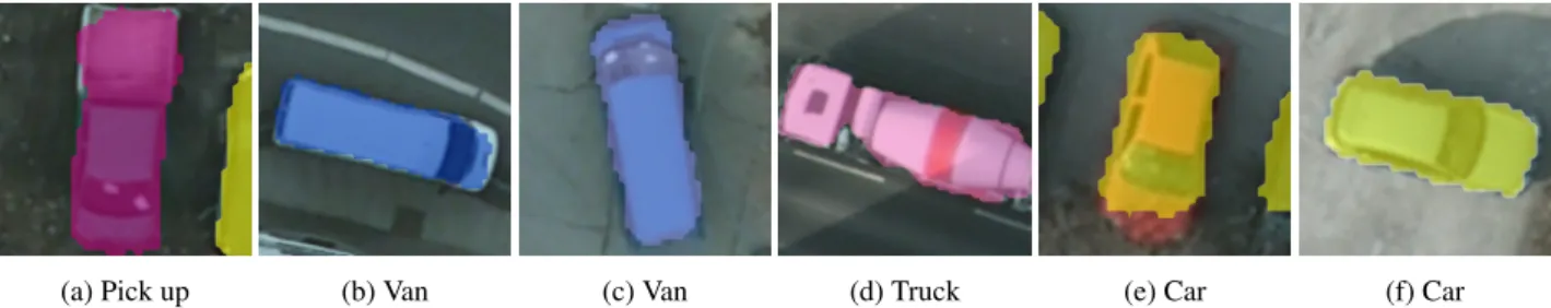
(a) Pick up (b) Van (c) Van (d) Truck (e) Car (f) Car
Figure 4. Successful segmentation and classification of vehicles in the Potsdam dataset
Table 2. Vehicle counts in testing tiles of ISPRS Potsdam
Tile # 2_11 7_12 3_11 5_12 7_10 Cars in ground truth 110 351 168 428 253
Predicted cars 115 342 182 435 257
This is supported by qualitative inspection of the semantic maps on car-heavy areas, such as the one presented in Figure 5.
The mean Intersection over Union (IoU) reaches 75.6%. How-ever, there is a high variance in the IoU depending on the specific surroundings of each car. Indeed, because of occlusions due to trees, the ground truth sometimes is labelled as tree even if the car is visible in the RGB image. This causes SegNet to misclas-sify (according to the ground truth) most of the pixels, resulting in a low IoU despite the visual quality of the segmentation. This phenomenon is illustrated by Figure 2. However, as SegNet man-ages to still infer the car’s contours, this should not impede too severely later vehicle extraction and classification.
Counting cars We extract the vehicle mask from the semantic map of Potsdam generated by SegNet. Each connected compo-nent is expected to be a vehicle instance. We count the number of predicted instances in each tile of the testing set. Detailed results are reported in Table 2 and show that our model can be used to estimate precisely the number of vehicles in the original tile with an average relative error of less than 4%.
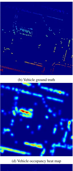
We also show that we can use this information to generate heat maps of the vehicle repartition in the tile (cf. Figure 6). Such a visualization provides an indicator of the vehicle density in the urban area, and exacerbates high traffic roads and “hot spots” cor-responding to parking lots around points of interest (e.g. hospitals or shopping malls). This can be useful for many urban planning applications, such as parking lot sizing, traffic estimation, etc. In temporal data, this could be used to monitor traffic flows, but also study the impact of the road blocks, jams, etc.
Classification Using our AlexNet-based CNN classifier, we are able to classify the candidate vehicle instances generated by Seg-Net on the Potsdam dataset. We compare the predicted results to our enhanced vehicle ground truth. On our testing set, we clas-sify correctly 75.0% of the instances. We are able to improve even further this result by switching to the VGG-16 based clas-sifier which brings accuracy to 77.3% (cf. Table 3 for detailed results). It should be noted that the dataset is predominantly comprised of cars, and that trucks and pick ups are less repre-sented, which decreases their influence on the global accuracy score. Figure 4 illustrates some vehicle instances where our deep network-based segmentation and classification pipeline was suc-cessful, while Figure 3 shows some examples of correct segmen-tation but subsequent misclassification.
The fact that the average accuracy of the models on Potsdam are lower than results reported on VEDAI suggests that our networks
Table 3. Classification results on the enhanced Potsdam vehicle ground truth
Class Car Van Truck Pick up Global AlexNet 81% 42% 50% 50% 75%
VGG 83% 55% 50% 33% 77%
suffered from overfitting. One hypothesis that we make is that VEDAI and Potsdam are images taken from two similar but sub-tly different environments. Indeed, Potsdam is a urban european city whereas VEDAI images have been shot over Utah, on a more rural american environment. Therefore, vehicle brands and dif-ferent land covers around the cars might influence the classifiers. More comprehensive regularization (e.g. dropout (Srivastava et al., 2014)) during fine-tuning and/or training on a more diverse dataset would help alleviate this phenomenon.
4. CONCLUSION
In this work, we presented a two-step framework to detect, seg-ment and classify vehicles from aerial RGB images using deep learning. More precisely, we showed that deep network designed for semantic segmentation such as SegNet are useful for scene understanding of remote sensing data and can be used to segment even small objects, such as cars and trucks. We reported results on the ISPRS Potsdam dataset showing very promising results on wheeled vehicles, achieving a F1 score of 77.3% on this specific class.
In addition, we presented a simple deep learning based method to improve further this analysis by classifying the different types of vehicle present in the scene. We trained several deep CNN on the VEDAI dataset and transferred their knowledge to the Potsdam dataset. Our best model, fine-tuned from VGG-16, was able to classify successfully more than 77% of the vehicles in our testing set.
Finally, this work meant to provide useful pointers for applying deep learning to scene understanding in Earth Observation with an object-oriented approach. We showed that not only deep net-works are the state-of-the-art for semantic mapping, but that they can also be used to extract useful information at an object level, with a direct application on vehicle detection and classification.
We showed that it is possible to enumerate and extract individual object instances from the semantic map in order to analyze the vehicle distribution in the images, leading to the localization of points of interest such as high traffic roads and parking lots. This has many applications in traffic monitoring and urban planning, such as analyzing parking lots occupancy, finding pollutants ve-hicles in unauthorized zones (combined with a classifier), etc.
(a) RGB data (b) Ground truth (c) SegNet prediction
Figure 5. SegNet results on a parking lot (extracted from the ISPRS dataset, best viewed in color)
ACKNOWLEDGEMENTS
The Potsdam data set was provided by the German Society for Photogrammetry, Remote Sensing and Geoinformation (DGPF): http://www.ifp.uni-stuttgart.de/dgpf/DKEP-Allg.html. The Vehicle Detection in Aerial Imagery (VEDAI) dataset was provided by S. Razakarivony and F. Jurie.
N. Audebert’ work is funded by ONERA-TOTAL research project Naomi.
The authors would like to thank A. Boulch and A. Chan Hon Tong for fruitful discussions on object detection and classification.
REFERENCES
Audebert, N., Le Saux, B. and Lefèvre, S., 2016. How Useful is Region-based Classification of Remote Sensing Images in a Deep Learning Framework? In: IEEE International Geosciences and Remote Sensing Symposium (IGARSS), Beijing, China.
Badrinarayanan, V., Kendall, A. and Cipolla, R., 2015. SegNet: A Deep Convolutional Encoder-Decoder Architecture for Image Segmentation. arXiv preprint arXiv:1511.00561.
Chen, X., Xiang, S., Liu, C. L. and Pan, C. H., 2014. Vehicle De-tection in Satellite Images by Hybrid Deep Convolutional Neural Networks. IEEE Geoscience and Remote Sensing Letters 11(10), pp. 1797–1801.
Cramer, M., 2010. The DGPF test on digital aerial camera evalu-ation – overview and test design. Photogrammetrie – Fernerkun-dung – Geoinformation2, pp. 73–82.
Everingham, M., Eslami, S. M. A., Gool, L. V., Williams, C. K. I., Winn, J. and Zisserman, A., 2014. The Pascal Visual Object Classes Challenge: A Retrospective. International Journal of Computer Vision111(1), pp. 98–136.
Ioffe, S. and Szegedy, C., 2015. Batch Normalization: Accel-erating Deep Network Training by Reducing Internal Covariate Shift. In: Proceedings of The 32nd International Conference on Machine Learning, pp. 448–456.
Krizhevsky, A., Sutskever, I. and Hinton, G. E., 2012. ImageNet Classification with Deep Convolutional Neural Networks. In: F. Pereira, C. J. C. Burges, L. Bottou and K. Q. Weinberger (eds), Advances in Neural Information Processing Systems 25, Curran Associates, Inc., pp. 1097–1105.
Lagrange, A., Le Saux, B., Beaupere, A., Boulch, A., Chan-Hon-Tong, A., Herbin, S., Randrianarivo, H. and Ferecatu, M.,
2015. Benchmarking classification of earth-observation data: From learning explicit features to convolutional networks. In: Geoscience and Remote Sensing Symposium (IGARSS), 2015 IEEE International, pp. 4173–4176.
Lecun, Y., Bottou, L., Bengio, Y. and Haffner, P., 1998. Gradient-based learning applied to document recognition. Proceedings of the IEEE86(11), pp. 2278–2324.
Liang-Chieh, C., Papandreou, G., Kokkinos, I., Murphy, K. and Yuille, A., 2015. Semantic Image Segmentation with Deep Con-volutional Nets and Fully Connected CRFs. In: Proceedings of the International Conference on Learning Representations.
Lin, T.-Y., Maire, M., Belongie, S., Hays, J., Perona, P., Ra-manan, D., Dollár, P. and Zitnick, C. L., 2014. Microsoft COCO: Common Objects in Context. In: D. Fleet, T. Pajdla, B. Schiele and T. Tuytelaars (eds), Computer Vision – ECCV 2014, Lecture Notes in Computer Science, Springer International Publishing, pp. 740–755. DOI: 10.1007/978-3-319-10602-1_48.
Long, J., Shelhamer, E. and Darrell, T., 2015. Fully Convolu-tional Networks for Semantic Segmentation. In: Proceedings of the IEEE Conference on Computer Vision and Pattern Recogni-tion, pp. 3431–3440.
Marmanis, D., Wegner, J. D., Galliani, S., Schindler, K., Datcu, M. and Stilla, U., 2016. Semantic Segmentation of Aerial Images with an Ensemble of CNNs. ISPRS Annals of Photogramme-try, Remote Sensing and Spatial Information Sciences3, pp. 473– 480.
Nogueira, K., Penatti, O. A. B. and Dos Santos, J. A., 2016. Towards Better Exploiting Convolutional Neural Networks for Remote Sensing Scene Classification. arXiv:1602.01517 [cs]. arXiv: 1602.01517.
Paisitkriangkrai, S., Sherrah, J., Janney, P. and Hengel, A. V.-D., 2015. Effective semantic pixel labelling with convolutional networks and Conditional Random Fields. In: Proceedings of the IEEE Conference on Computer Vision and Pattern Recognition Workshops, pp. 36–43.
Penatti, O., Nogueira, K. and Dos Santos, J., 2015. Do deep features generalize from everyday objects to remote sensing and aerial scenes domains? In: Proceedings of the IEEE Conference on Computer Vision and Pattern Recognition Workshops, pp. 44– 51.
Razakarivony, S. and Jurie, F., 2016. Vehicle Detection in Aerial Imagery: A small target detection benchmark. Journal of Visual Communication and Image Representation34, pp. 187–203.
(a) RGB data (b) Vehicle ground truth
(c) Predicted vehicles (d) Vehicle occupancy heat map
(e) RGB data (f) Vehicle ground truth
(g) Predicted vehicles (h) Vehicle occupancy heat map
Rottensteiner, F., Sohn, G., Jung, J., Gerke, M., Baillard, C., Ben-itez, S. and Breitkopf, U., 2012. The ISPRS benchmark on urban object classification and 3d building reconstruction. ISPRS Ann. Photogramm. Remote Sens. Spat. Inf. Sci1, pp. 3.
Russakovsky, O., Deng, J., Su, H., Krause, J., Satheesh, S., Ma, S., Huang, Z., Karpathy, A., Khosla, A., Bernstein, M., Berg, A. C. and Fei-Fei, L., 2015. ImageNet Large Scale Vi-sual Recognition Challenge. International Journal of Computer Vision115(3), pp. 211–252.
Simonyan, K. and Zisserman, A., 2014. Very Deep Convolutional Networks for Large-Scale Image Recognition. arXiv:1409.1556 [cs]. arXiv: 1409.1556.
Srivastava, N., Hinton, G., Krizhevsky, A., Sutskever, I. and Salakhutdinov, R., 2014. Dropout: A simple way to prevent neural networks from overfitting. J. Mach. Learn. Res. 15(1), pp. 1929–1958.