Publisher’s version / Version de l'éditeur:
Vous avez des questions? Nous pouvons vous aider. Pour communiquer directement avec un auteur, consultez la première page de la revue dans laquelle son article a été publié afin de trouver ses coordonnées. Si vous n’arrivez Questions? Contact the NRC Publications Archive team at
[email protected]. If you wish to email the authors directly, please see the first page of the publication for their contact information.
https://publications-cnrc.canada.ca/fra/droits
L’accès à ce site Web et l’utilisation de son contenu sont assujettis aux conditions présentées dans le site LISEZ CES CONDITIONS ATTENTIVEMENT AVANT D’UTILISER CE SITE WEB.
10th Conference on Building Science and Technology Proceedings, 2, pp. 32-41,
2005-05-01
READ THESE TERMS AND CONDITIONS CAREFULLY BEFORE USING THIS WEBSITE.
https://nrc-publications.canada.ca/eng/copyright
NRC Publications Archive Record / Notice des Archives des publications du CNRC : https://nrc-publications.canada.ca/eng/view/object/?id=fdc5cb7e-053c-44d8-8934-a6773b131aff https://publications-cnrc.canada.ca/fra/voir/objet/?id=fdc5cb7e-053c-44d8-8934-a6773b131aff
NRC Publications Archive
Archives des publications du CNRC
This publication could be one of several versions: author’s original, accepted manuscript or the publisher’s version. / La version de cette publication peut être l’une des suivantes : la version prépublication de l’auteur, la version acceptée du manuscrit ou la version de l’éditeur.
Access and use of this website and the material on it are subject to the Terms and Conditions set forth at
Hygrothermal performance of building envelopes: uses for 2D and 1D
simulation
Hygrothermal performance of building envelopes:
uses for 2D and 1D simulation
Dalgliesh, A.; Cornick, S.; Maref, W.;
Mukhopadhyaya, P.
NRCC-48156
A version of this document is published in / Une version de ce document se trouve dans :
10
thConference on Building Science and Technology Proceedings,
Ottawa, Ont., May 12-13, 2005, v. 2, pp. 32-41
Hygrothermal Performance of Building Envelopes:
Uses for 2D and 1D simulation
Alan Dalgliesh1, Steve Cornick2, Wahid Maref 2and Phalguni Mukhopadhyaya2
ABSTRACT
A building’s durability depends on controlling heat and moisture within its envelope. Moisture diffuses through porous materials that may suffer mould growth and decay (if wood-based) when left moist and warm for too long. Designers try to keep vulnerable components dry, but materials can start to deteriorate before reaching the dew point temperature. Researchers use two-dimensional hygrothermal modeling to calculate time-varying moisture content and temperature at points on a plane through the building envelope thickness.
One-dimensional versions of several research programs have been written to assist designers and other building envelope specialists in their work. This paper compares moisture and temperature histories in two building envelopes exposed to a variety of climatic conditions over three years, as calculated by 2D and 1D versions of one such computer program. The 2D calculations come from reports on a methodology for moisture management of wood-frame walls, published in 2003 by a consortium of industry and research partners. Results for a face-sealed stucco wall with rain entry by diffusion only (no seal deficiencies) showed reasonable agreement between 2D and 1D, whereas those for a brick wall with a ventilated air space diverged considerably. With due respect for limitations, 1D simulation can give a first
indication of the differences in performance of a wall exposed to different climates, or between different wall assemblies. In some cases the user should consider following up with 2D simulation or field monitoring.
INTRODUCTION
Acceptable hygrothermal performance of building envelopes cannot always be taken for granted. In the mid 1990's, residential designs and construction techniques with adequate track records in relatively dry climates began to fail prematurely in great numbers in wet coastal climates. Investigators reported that rain leaks at through-wall penetrations caused 90% of the damage found in their study of 37 condos on the lower mainland of coastal BC. Three rain management strategies (face seal, weather barrier with drainage plane, rain screen, each of which exhibited failures) had been used, in a climate with 5 times the rain, 4 times the wind-driven rain index, and only 1/3 the hours of sunshine of most inland communities in Canada. [1] Designers, building code officials and inspectors, developers, contractors and materials suppliers, even research institutions and lending agencies, all came under fire over the heavy losses suffered by owners and tenants in the Vancouver area. Mould and wood rot were common features of the damage resulting from extended periods of wetness inside walls.
Designers sometimes use steady-state calculations to predict dew point temperatures at critical points through the thickness of the wall, on the assumption that condensation would signal the onset of mould or wood rot. It now appears that such organisms will germinate and grow at relative humidities (RH) over 80 percent for temperatures (T) over 5 °C. [2] To predict time-varying RH and T throughout a wall section, researchers use hygrothermal modeling programs that require input files of material properties, hourly weather records, and considerable expertise to operate. [3, 4, 5] In many investigations two-dimensional (2D) grids are required as well. “User-friendly” 1D versions of research programs are now available for practitioners to become familiar with the hygrothermal performance of building envelopes. [6, 7] Material properties and weather files are provided, which simplifies the preparation of a simulation run. The simulation takes only a fraction of the time needed for a 2D run, and output quantities such as RH and T can be displayed graphically for easy comparisons of performance between different wall assemblies, or for different climates.
1
Corresponding author,
consultant, 237 Valley Ridge Green NW, Calgary AB T3B 5L6, phone 403-286-2177[email protected]
2Research Officers, Institute for Research in Construction, National Research Council of Canada, 1200 Montreal Road, Ottawa, ON, K1A 0R6
A practitioner will find such a program easier to use than a full-blown research program (1D or 2D), but still has to acquire a certain level of expertise before applying the results to practical problems, and must learn which problems can be handled by a 1D simulation. In 2003, a research consortium published a study of moisture management for building envelopes in a range of North American climates. [8] The authors of this paper selected some of the consortium’s 2D simulations and redid them, using a 1D version of the same program. Our purpose was to find out the extent to which 1D simulation might be considered useful for generating insights consistent with the original findings, but in addition, we would like to comment on some of the uncertainties facing users of both 1D and 2D programs.
MOISTURE MANAGEMENT – FINDINGS OF A RESEARCH CONSORTIUM:
The consortium worked out a method for predicting the moisture management performance of walls as a function of climate severity, in which hygrothermal modeling played a central role. A 2D program was used to solve the equations of conservation of mass and energy governing the flow of heat, air and moisture, to track temperature and moisture content in four generic building envelope assemblies. Two of the four wall assemblies are shown in Figure 1. The consortium's final report [9] gives designers and other non-researchers insight on what moisture-handling performance to expect from a few different wall designs exposed to a range of North American climates, but cautions readers to consult the research team before applying the information to building designs. Interested readers should consult the report for a full description; the purpose here is limited to identifying those 2D simulation cases suitable for comparison with 1D simulation.
Modeling rain leakage – not feasible for 1D simulation:
The findings of the B.C. condo study made leakage paths a major factor in the research project. Full-scale walls with deliberately created paths were exposed (in lab tests) to water sprays and air pressure differences simulating driving rain. Water entering the stud space was expressed as a function of spray rate (amount of rain hitting the wall/hour) and air pressure (average wind pressure during the hour). The fitted relations found for each wall and deficiency type were then used to calculate quantities of water that were injected, as point sources, into the stud spaces for most of the hundreds of 2D simulations.
Moisture from point sources can diffuse up or down in a 2D simulation as well as horizontally, which is the only option for 1D. With the possible exception of a vertical array of uniform point sources, the authors believe that simulation of rain leakage is not feasible for 1D. This is the first major difference in capability between 2D and 1D programs.
FIGURE 1
SELECTION OF FOURTEEN 2D CASES FOR COMPARISON TO 1D:
Several different configurations of material properties were simulated for each of the four wall systems. One set of material properties was selected as the reference wall, and with no injections of leakage moisture, functioned as a base case. In the base cases, liquid and vapour entered by diffusion processes only, making them candidates for 1D simulation. Even without leakage paths, rain striking the wall played a major role in the ingress of moisture for the base cases. Of the four generic wall assemblies, the most suitable was the stucco wall, for two reasons: 1) it contained no ventilated air space, and 2) in the early stages of the parametric study, histories of moisture content and temperature averaged over vertical grid points for the bottom 600 mm of the interior face of the OSB sheathing were available. Unfortunately for our investigation, however, the region of interest was later switched to the grid points on 50 mm of the top of the bottom plate, which is spruce and not OSB.
The brick wall (results available for the spruce plate only) was selected to show the greatest differences between 2D and 1D, thus rounding out the study to cover 14 base case simulations: two wall assemblies exposed to seven climates.
Weather records and material properties:
1D hygIRC includes a database containing weather files, with the same records used in the 2D simulations for the consortium (see Table 1). In 2D, a preliminary year of conditioning with the so-called “wet” year was followed by a repetition of the wet year and the average year. The latter two years were used to examine RH and T, and those 2D results will be compared to 1D simulations using the same combinations of years of weather record.
TABLE 1
Weather Records for 2D and 1D Simulations
City wet year average year City wet year average year
Phoenix AZ 1978, East 1979, East Winnipeg MB 1968, North 1978, North Fresno CA 1982, East 1980, East Ottawa ON 1969, East 1959, East San Diego CA 1983, South 1982, South Seattle WA 1990, South 1984, South
Wilmington NC 1984, North 1988, North East
The algorithm recommended by Straube [10] is used to convert hourly rainfall on the ground (Rh) to rain hitting the wall (Rv). For current developments in this area, see Blocken and Carmeliet’s review of wind-driven research and its implications for hygrothermal modeling [11] :
Rv = RAF•DRF•cos(Ԧ)•Vz• Rh, where
x Rain Admittance Factor RAF = 0.4 for the mid-height of a low building wall (~2m);
x Driving Rain Factor DRF = 1/Vt, the terminal velocity of raindrops, a function of their diameter; x Ԧ is the angle between the normal to the wall and the wind direction;
x Vz = V•(1.8/10)0.22, in which V is the weather file wind speed at a height of 10 m in open terrain.
The material properties in the 1D program’s database does not have precisely the same properties for some of the materials used in the consortium simulations, so their specifications were imported and used to eliminate potential sources of disagreement. The arrangements of materials for the two wall types, stucco and brick, are shown in Figure 1.
Number of nodes, initial and boundary conditions:
Moisture content and temperature are computed at several nodes in both the 1D and 2D programs with similar numbers and spacing per layer in the horizontal direction (e.g. 10 nodes in the OSB). Initial temperature and relative humidity were constant across all layers, but had little influence as the whole first year of simulation was used to acclimatize the assembly for calculations during the second and third years. Boundary conditions, however, were found to be rather influential, and those of the 2D simulations differed from the 1D program’s default values (for which ASHRAE was a likely source [12]). The 1D simulations reported in this paper were run using the same boundary conditions as the 2D simulations:
2D simulation 1D default values x heat transfer coefficients, exterior and interior 10 w/m²•K 30 exterior, 8 interior x moisture transfer coefficients, exterior and interior 7.4 x 10⁻⁸ kg/m²•s•Pa 21 exterior, 5.9 interior x absorptivity and emissivity (exterior) 0.8 and 0.9 0.5 and 0.9
Relative Humidity and Temperature Comparisons – Stucco wall:
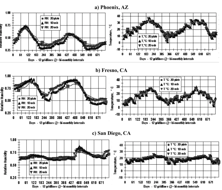
Figure 2 displays five different climate types: 1) Phoenix, hot and dry; 2) Fresno and San Diego, warm and dry; 3) Winnipeg, cold and dry; 4) Ottawa, cold and wet; 5) Seattle and Wilmington, mild and wet. For ease of comparisons, the scales are the same for all graphs of RH, and the scales for graphs of Temperature run from -10 to 45 C except those for Winnipeg and Ottawa, which had to be shifted down by 20 C. Two year averages of RH for the 1D OSB node next to the insulation came within 4 percent of the 2D OSB “region of interest” for all seven climates (see statistics in Table 2).
The third curve in each graph, giving 2D results for the spruce plate (under the generally dryer insulation), might be expected to indicate lower moisture contents than the other two, and in fact the average RH values are lower by 9 percent for Seattle, 14 percent for Ottawa, and 19 percent for Winnipeg. What is more surprising is that the values for Fresno, San Diego, and Wilmington are all within 3 percent of the OSB values, and that for Phoenix is actually 8 percent higher.
FIGURE 2
: left) RH Vs. time and right) Temperature Vs. time for the Stucco wall
a) Phoenix, AZ
b) Fresno, CA
d) Winnipeg, MB
e) Ottawa, ON
f) Seattle, WA
Relative Humidity and Temperature Comparisons – Brick wall:
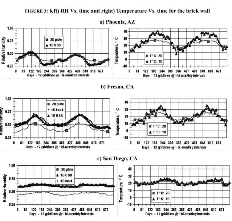
The scales for all graphs are the same as those in Figure 2. RH and T data available from the 2D simulation of the brick wall referred only to the bottom plate. It seemed likely that the plate RH and T might correspond more closely to the RH and T calculated for a node point in the glass fibre insulation layer, rather than to the right-most node of the OSB. This turned out to be the case for only three climates: Ottawa, Seattle, and Wilmington, as shown by the 1D result for node 33, second from the left in the insulation (with diamond markers). Fresno and San Diego appeared to be candidates for a better fit with the insulation, but there was very little difference between the two 1D simulations, and for whatever reason, the 1D OSB results matched the 2D plate results fairly well for Phoenix and Winnipeg, so no insulation results are shown for them. The 2D simulation included heat, air and moisture exchanges with the exterior through venting slots into the air space. The ventilation gaps can just be seen at the top and bottom interior edges of the brick in the right-hand wall of Figure 1. The air space in the 1D simulation could not model such exchanges, a second major difference in capability between 2D and 1D.
FIGURE 3
: left) RH Vs. time and right) Temperature Vs. time for the brick wall
a) Phoenix, AZ
b) Fresno, CA
d) Winnipeg, MB
e)
Ottawa, ON
f)
Seattle, WA
DISCUSSION OF 1D TO 2D COMPARISONS OF RH AND T:
General observations:
Top and bottom plates are the most obvious non-uniform features in the vertical direction of the walls. For the stucco wall, 2D calculations for nodes on horizontal slices midway up the wall were expected to agree quite well with 1D, except perhaps for gravitational effects. Early in the 2D simulations, RH and T results were compiled as averages of the vertical nodes in the bottom 600 mm (1/4 if the wall height), at the interior surface of the OSB. These results, taken at 10-day intervals for a total of 73 values in the last two years of the simulation, compared surprisingly well to the 1D simulations; in fact, for each of the seven cities, 1D and 2D average RH values are virtually identical (Table 2). Concerning 1D to 2D comparisons of T, we expected them to be good (better than for moisture content), but noticed greater seasonal swings for Winnipeg, and in the case of the brick wall, all cities except San Diego, Seattle, and Wilmington. We don’t have an explanation for those discrepancies.
Two additional problems were expected for the brick wall. First, the only results available for comparison referred to the bottom plate, an element that could not be modeled except in 2D. Second, the ventilated air space of the brick wall was expected to introduce heat, air, and moisture transfers between the space and the exterior that could not be represented in 1D either. All in all, the prospects for the 7 brick wall simulations didn’t seem promising. Although certainly less close and less consistent than the agreements found for the stucco wall, the 1D simulations for the brick wall did share a fair number of the trends and features with the 2D simulations.
Our first attempts were discouraging because we failed to ensure that a) algorithms internal to the 1D program would produce driving rain appropriate to the 1.8 m height used in the 2D simulation, and b) heat and mass transfer coefficients at the boundaries in the 1D program agreed with those used in the 2D simulation. At a rough guess, these two errors each added about 10 or 15 percent to the moisture contents calculated, so it was a great relief when these errors were rectified.
Lowering the moisture transfer coefficient for the air layer at the exterior boundary from 21E-8 kg/m2•s•Pa to 7.4E-8kg/m2•s•Pa significantly reduces the amount of rainwater that finds its way into the sheathing. Putting moisture sources near the bottom plate to represent leakage for the 2D simulations had the opposite effect. The fact that one can lower or raise the ingress of moisture due to rain by manipulating conditions at the exterior boundary or within the wall reminds us that even if agreement is found between measurements from a real wall and a particular simulation (or for that matter, between two different simulations), the reasons for agreement may be different than we think, and quite possibly not legitimate. The sensitivity of results to boundary conditions underscores the need to justify them along with all other input conditions, both for 2D and 1D simulation.
Many researchers regard RH and T values as relative, not absolute indications of performance, and with that proviso, the RH and T comparisons suggest that 1D and 2D users will generally rank climate severity, or alternatively the performance of different walls in a given climate, in the same order. The comparisons made in this study suggest that 1D simulation, while showing similar trends, may give higher numerical values of RH, apparently through higher moisture levels rather than lower temperatures. This should not be a problem when considering relative differences, but may be of concern for more sophisticated uses involving damage functions to predict, not just the onset, but also the progressive growth of moulds or decay fungi. [2]
Given its relative speed, economy, and ease of operation, 1D simulation might usefully serve as a precursor to commissioning of 2D simulation when circumstances seem to call for hygrothermal modeling. But even if 1D and 2D simulations lead to similar recommendations for the building envelope, there is no guarantee that the simulations are close enough to the real situation to be useful. As one example, although rain leakage will be a major concern in many practical investigations, researchers are only now making stabs at allowing for its effect. Even in 2D, the leakage paths are not simulated; supplementary investigations or assumptions are used to dictate when, where, and how much moisture is injected inside the wall. In other words, benchmarking against observations in the field is required to close the loop between simulations and practical problems.
Elementary statistical measures:
Table 2 brings together minimum, maximum, and average values computed over the two-year simulation for each of the seven climates and two wall assemblies. Although magnitudes differ, directions of changes in RH from city to city, or from stucco to brick are nearly always the same for 1D and 2D results. This is the justification for stating that 1D and 2D simulations were found to share the same trends in performance prediction.
TABLE 2
Statistics of 1D and 2D RH Calculations for Stucco and Brick Walls in Seven Cities
Phoenix Fresno San Diego Winnipeg Ottawa Seattle Wilmington Statistic, Wall Type
1D 2D 1D 2D 1D 2D 1D 2D 1D 2D 1D 2D 1D 2D Stucco .278 .322 .432 .499 .606 .622 .686 .700 .732 .770 .829 .879 .785 .843 Minimum RH in two years Brick .271 .342 .438 .352 .594 .420 .638 .573 .335 .392 .408 .430 .478 .431 Stucco .741 .689 .946 .909 .869 .872 .866 .876 .902 .891 .960 .937 .970 .966 Maximum RH in two years Brick .535 .480 .692 .547 .643 .493 .827 .696 .763 .609 .854 .614 .867 .574 Stucco .435 .454 .708 .731 .671 .683 .771 .769 .818 .834 .910 .910 .933 .937 Average RH over
two years Brick .385 .394 .548 .433 .618 .459 .699 .647 .526 .487 .619 .514 .692 .494
Stucco -4% -3% -2% 0% -2% 0% 0%
1D - 2D 0.01•2D
Ave. RH Brick -2% 27% 35% 8% 8% 20% 40%
SUMMARY AND CONCLUDING REMARKS:
1D and 2D RH and T results for the stucco wall show similar trends of performance as a function of climate severity. Histories of temperature were in fairly good agreement for all 14 cases examined, but the 1D calculations of relative humidity were significantly higher than the 2D calculations in 4 of the 7 cases involving the brick wall. One is tempted to attribute this conservative result for 1D to its inability to compensate effectively for convective exchange of moisture and heat across vented air spaces. Non-uniformity in the vertical direction (top and bottom plates) appeared to have less influence than anticipated, since 1D and 2D were in good agreement for the stucco wall in all 7 climates. It would be interesting to run 2D simulations of the base case (no moisture sources in the wall) with the spruce plates removed, to investigate this apparent insensitivity further.
Neither 1D nor 2D simulations, even if they chance to agree, will be persuasive for building envelope specialists if the simulation predictions appear to run counter to their own practical experience. Field monitoring designed to test the reliability of hygrothermal modeling seems to be the most direct way to resolve such differences. Another important area for improvement is the characterization of building material properties, including their statistical scatter. Benchmarking based on laboratory tests allow a much higher standard of agreement, but for applications to real-world problems, it appears that to expect differences of no more than 20 percent in, say, moisture content estimates might be considered optimistic.
When doing simulations involving weather records, one must be quite clear about the method used to convert rainfall and wind effect into moisture on the wall, where it can be absorbed through porous cladding or be moved by air pressure and gravity through leakage paths. The algorithm used by the 1D program applies to low buildings; if modified for cladding near the top of a 10-storey building, moisture intake from rain can be expected to increase by upwards of 15 percent. Complex phenomena are involved in the deposition of rainwater on walls, which affect 2D just as much as 1D simulation, but the good news is that coordinated research efforts [11] are starting to bridge this particular gap between simulation and natural events.
Another work in progress concerns the choice of representative weather records, a major source of variability in results. Opinion seems divided on whether to use rainfall, temperature, or some combination of the two as the main criterion. Different choices might be appropriate, depending on the damage mechanism at work (freeze-thaw or wetting-drying cycles for example). Until greater confidence in exterior boundary conditions is warranted, one should be prepared for substantial discrepancies between simulation results and field performance (added to the 20 percent mentioned already).
Moisture management requires a clear understanding of the moisture loading on the building envelope. Hygrothermal models are continually improving, and allow researchers and practitioners alike to make predictions based on the best information available on material properties and climatic conditions. Though water and air movement through leaks are of major practical importance, leakage paths are not currently amenable to simulation even by 2D programs. When applicability is questionable for either 1D or 2D simulation, field monitoring should be given serious consideration.
1D simulation’s most attractive features are ease of use, economy and above all, short time frames for investigating problems that would otherwise never be given such close attention. Although the corresponding author found the learning curve steeper than expected, the effort was more than repaid by these advantages.
REFERENCES
[1] Canada Mortgage and Housing Corporation. 1996. Survey of Building Envelope Failures in the Coastal Climate of British Columbia. Submitted by Morrison Hershfield Limited, Suite 247, 4299 Canada Way, Burnaby, B.C. V5G 1H3 [2] Sedlbauer, K. 2002. Prediction of Mould Growth by Hygrothermal Calculation. Journal of Thermal Envelope and
Building Science, Vol. 25, No. 4, 321-336
[3] Nofal, Mostafa; Straver, Michelle and Kumaran, Kumar. 2001. Comparison of four hygrothermal models in terms of long-term performance assessment of wood-frame constructions. Proceedings of the Eighth Conference on Building Science and Technology, February 2001 pp. 118-138
[4] Karagiozis, Achilles and Desjarlais, André O. 2003. What Influences the Hygrothermal Performance of Stucco Walls in Seattle. Proceedings of the Ninth Conference on Building Science and Technology, February 2003 pp. 31-44
[5] Häupl, Peter. 2003. Quantification of the Hygrothermic Behaviour of Building Envelopes. Proceedings of the Ninth Conference on Building Science and Technology, February 2003 pp. 551-567
[6] Karagiozis, Achilles; Künzel, Hartwig and Holm, Andreas. 2001. WUFI/ORNL/IBP Hygrothermal Model. Proceedings of the Eighth Conference on Building Science and Technology, February 2001 pp. 158-183
[7] Cornick, Steve; Maref, Wahid; Abdulghani, Khaled and David van Reenen. 2003. 1-D hygIRC: A Simulation Tool for Modeling Heat, Air and Moisture Movement in Exterior Walls. Building Science Insight 2003 Seminar Series, Effective Moisture Control for Light-Frame Walls of Low-Rise Buildings 10 pages
[8] Kumaran, M.K.; Mukhopadhyaya, P.; Cornick, S.M.; Lacasse, M.A.; Rousseau, M.; Maref, W.; Nofal, M.; Quirt, J.D. and Dalgliesh, W.A. 2003. An Integrated Methodology to Develop Moisture Management Strategies for Exterior Wall Systems. Proceedings of the Ninth Conference on Building Science and Technology, February 2003 pp.45-62
[9] Beaulieu, P. et al. 2002. Hygrothermal Response of Exterior Wall Systems to Climate Loading: Methodology and Interpretation of Results for Stucco, EIFS, Masonry and Siding-clad Wood-frame Walls. Research report 118, Institute for Research in Construction , National Research Council Canada, Ottawa Canada K1A 0R6.
[10] Straube, J.F., 1998. Moisture Control and Enclosure Wall Systems. Ph.D. Thesis, Civil Engineering Department, University of Waterloo Chapter 5, “Rain, Driving Rain, and Enclosure Walls”
.
[11] Blocken, Bert and Jan Carmeliet, 2004
.
A review of wind-driven rain research in building science. Journal of Wind Engineering and Industrial Aerodynamics 92 (2004) 1079-1130.[12] American Society of Heating, Refrigerating and Air Conditioning, 1989