Analytic calculations of MHD equilibria and of MHD stability boundaries in fusion plasmas

Analytic calculations of MHD equilibria and of MHD

stability boundaries in fusion plasmas

by

2

Antoine Julien Cerfon

B.S. Mathematics and Physics (2003), M.S. Nuclear Science and Engineering (2005) Ecole Nationale Superieure des Mines de Paris

Submitted to the Department of Nuclear Science and Engineering in partial fulfillment of the requirements for the degree of

Doctor of Philosophy in Applied Plasma Physics at the

MASSACHUSETTS INSTITUTE OF TECHNOLOGY September 2010

@ Massachusetts Institute of Technology 2010. All rights reserved.

A u th o r ... .. ... ... Department of Nuclear Science and Engineering

August 24, 2010

Certified by...

(....Jeffrey P. Freidberg

KEPCO Professor of Nuclear Science and Engineering Department

A Thesis Supervisor

Certified by ...

V

Senior Research Scientist, Plasma Science and Fusion Center Thesis Reader

Accepted by...

LI Mujid S. Kazimi TEPCO Professor of Nuclear Science and Engineering Department

Analytic calculations of MHD equilibria and of MHD

stability boundaries in fusion plasmas

by

Antoine Julien Cerfon

Submitted to the Department of Nuclear Science and Engineering on August 25, 2010 in partial fulfillment of the requirements for the Degree of

Doctor of Philosophy in Applied Plasma Physics

Abstract

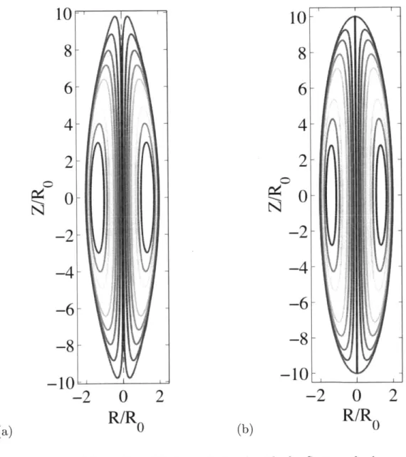
In this work, two separate aspects of ideal MHD theory are considered. In the first part, analytic solutions to the Grad-Shafranov equation (GSE) are presented, for two families of source functions: functions which are linear in the flux function T , and functions which are quadratic in T. The solutions are both simple and very versatile, since they describe equilibria in standard tokamaks, spherical tokamaks, spheromaks, and field reversed configurations. They allow arbitrary aspect ratio, elongation, and triangularity as well as a plasma surface that can be smooth or possess a double or single null divertor X-point. The solutions can also be used to evaluate the equilibrium beta limit in a tokamak and spherical tokamak in which a separatrix moves onto the inner surface of the plasma.

In the second part, the reliability of the ideal MHD energy principle in fusion grade plasmas is assessed. Six models are introduced, which are constructed to better describe plasma collisonality regimes for which the approximations of ideal MHD are not justified. General 3-D quadratic energy relations are derived for each of these six models, and compared with the ideal MHD energy principle. Stability comparison theorems are presented. The main conclusion can be summarized in two points. (1) In systems with ergodic magnetic field lines, ideal MHD accurately predicts marginal stability, even in fusion grade plasmas. (2) In closed field line geometries, however, the ideal MHD predictions must be modified. Indeed, it is found that in collisionless plasmas, the marginal stability condition for MHD modes is inherently incompressible for ion distribution functions that depend only on total energy. The absence of compressibility stabilization is then due to wave particle resonances. An illustration of the vanishing of plasma compressibility stabilization in closed line systems is given by studying the particular case of the hard-core Z-pinch.

Thesis Supervisor: Jeffrey P. Freidberg

Acknowledgments

I have long known that no matter where you are, you always find someone who is smarter than you. I just never thought that at MIT, this would be true in each and every office, and each and every classroom. It is quite a luxury to be going to work every day knowing that one will be challenged, and looking forward to all the new things one will learn. I wish I could thank all the people I met in labs or classrooms during my time here.

My first thanks go to all the fantastic people I met and worked with at PSFC. To Jeffrey Freidberg, who gave me the opportunity to join the theory group, and who introduced me and guided me through really fun projects; my answer to the question " _{Are you happy or sad?" is unequivocal. To Peter Catto, with whom I}

never managed to go to an Irish music concert, but from whom I learned so much about transport, and who always had very interesting comments and suggestions to help improve this work. To Rick Temkin, for letting me join PSFC in the first place, and giving us so many useful tips about the art of scientific presentation (I still need practice, though...). To Felix and his encyclopedic knowledge. To Grisha, for teaching me the jumping relaxation techniques. To Matt, for being so thorough, and never letting any argument convince him too easily. To Arturo, and his always dangerous visits in the office. To Antonio, for our shared passion for soccer, err football. To Dave, for teaching me about hockey. To Haru, for coming so often to my concerts. To Abhay, Jay, John, Paul, Darin and Ted for the interesting conversations at lunch time.

More personally, Miranda, thank you so much for embarking with me on this beautifully crazy (and crazily beautiful) adventure, and for sharing my belief that we would make it.

Brice, Thom, Steve,

j'espere

Edith, je te remercie du fond du coeur pour la curiosit6 que tu m'as g6netiquement l6gu6e, puis consciemment transmise.

Contents

1. Introduction...

11

2. Static MHD equilibria and analytic solutions to the Grad-Shafranov equation ... 25

2.1 Confined plasma equilibrium and Grad-Shafranov equation... 27

2.1.1 Equilibrium equations in fusion plasmas ... 27

2.1.2 Equilibrium in toroidally axisymmetric plasmas: the Grad-Shafranov eq u a tio n ... 3 2 2.2 Analytic solutions of the Grad-Shafranov equation with Solov'ev profiles... 38

2.2.1 Analytic solutions of the Grad-Shafranov equation... 38

2.2.2 The Grad-Shafranov equation with Solov'ev profiles ... 41

2.2.3 The boundary constraints... 46

2.2.4 The plasm a figures of m erit... 51

2 .2 .5 IT E R ... . . 5 3 2.2.6 T he spherical tokam ak ... 54

2.2.7 T he spherom ak ... 60

2.2.8 The field reversed configuration ... 61

2.2.9 Up-down asymmetric formulation ... 65

2.3 Extension: Analytic solutions of the Grad-Shafranov equation with quadratic p ro file s ... 6 9 2.3.1 Solov'ev profiles and the discontinuity of the toroidal current density... 69 2.3.2 Analytic solution of the Grad-Shafranov equation with quadratic profiles. 71

2.3.3 Up-down symmetric solutions... ₇₄

2.3.4 Up-down asymmetric solutions... 76

2 .4 S u m m ary ... . . 79

3. Are fusion plasmas compressible? A new look at MHD comparison

theorems ...

₈₅

3.1 Ideal MHD linear stability and the ideal MHD energy principle ... 87

3.1.1 Ideal M H D linear stability... ₈₇

3.1.2 Ideal MHD variational formulation ... 91

3.1.3 Ideal M H D energy principle ... 96

3.2 Ideal MHD plasma compressibility ... 99

3.3 Collisionality regimes in plasmas of fusion interest and alternate MHD models ... _{1 0 5} 3.4 Five models, one general formulation... 113

3.5 Two-Temperature MHD energy principle... 115

3.5.1 E lectron energy equation ... 116

3.5.2 Ion energy equation ... 121

3.5.3 Two-Temperature MHD static equilibrium... 122

3.5.4 Two-Temperature MHD stability and energy principle... 123

3.6 CGL - Fluid MHD energy principle ... 126

3.6.1 C G L - Fluid M H D closure ... ₁₂₆

3.6.2 CGL - Fluid MHD static equilibrium ... 128

3.6.3 CGL - Fluid MHD stability and energy principle... 129

3.7 Kinetic -Fluid M lD energy principle ... 133

3.7.1 K inetic - Fluid M H D closure... 133

3.7.2 Kinetic - Fluid MHD equilibrium... ₁₃₅

3.7.3 Kinetic - Fluid MHD energy principle ... ₁₃₆

3 .8 .1 C G L clo su re... 14 2

3.8.2 C G L static equilibrium ... 143

3.8.3 CGL stability and energy principle ... 144

3.9 Kinetic MHD energy principle ... 146

3.9.1 The Kinetic MHD closure... 146

3.9.2 Kinetic MHD static equilibrium ... 148

3.9.3 Kinetic MHD energy principle... 149

3.10 Energy relations for comparison theorems: Vlasov ions, fluid electrons ... 155

3.10.1 T he electron m odel... 157

3.10.2 The Vlasov-Fluid model ... 158

3.10.3 Vlasov-Fluid Equilibrium ... 159

3.10.4 V lasov-F luid Stability ... 161

3 .1 1 S u m m ary ... 164

4. The vanishing of MHD compressibility stabilization: illustration in the

hard-core Z-pinch

...

173

4.1 LDX and the hard-core Z-pinch... 175

4.1.1 The Levitated Dipole experiment (LDX)... 175

4.1.2 T he hard-core Z-pinch ... 181

4.2 Ideal MHD stability of the interchange mode in the hard-core Z-pinch... 184

4.3 Vlasov-Fluid stability of the interchange mode in the hard-core Z-pinch... 188

4.3.1 Previous kinetic studies of the interchange mode in Z-pinch and point d ip ole geom etries... 18 8 4.3.2 Vlasov-fluid stability analysis... 192

4.3.3 The vanishing of MHD compressibility stabilization: a numerical example ... 2 0 3 4.3.4 Local approximation vs. global eigenvalue equation... 210 4 .4 C o n clu sio n ... 2 15

5. Summ ary and Conclusions...221

Appendix A. Kinetic MHD Energy Relation...225

Appendix B. Kinetic MHD Ions, Fluid Electrons Energy Relation...240

Chapter 1

Introduction

The ideal MHD model is perhaps the simplest description of neutral plasmas

one can think of. It is defined by the following set of equations:

OP _!1.(P )--V-(pv) =0 at dv p -= JxB- Vp dt d _p = 0 (1.1) di p V x B= ptJ Vx vx B) at

In eq. (1.1), p is the mass density of the plasma, v its velocity, and p its pressure.

J is the current flowing in the plasma, and B the magnetic field. Because of its

simplicity, and its somewhat surprising ability to accurately predict the macroscopic

behavior of plasmas, ideal MHD is the model most commonly used in the early stages

of the design of a magnetic fusion experiment. This early design phase is usually

missions of ideal MHD theory for magnetic fusion applications. First, one determines

an equilibrium state consistent with the steady-state version of eq. (1.1). Then, one

analyzes the perturbations around that equilibrium state, which are either stable

waves or instabilities. Among other considerations, the desirable equilibria are those

where the plasma is confined at a high pressure, and where major instabilities,

potentially leading to the eventual loss of plasma confinement, cannot be excited.

In this thesis, we look separately at each of the two cornerstones of ideal MHD

theory. In the first part, we calculate plasma equilibria in toroidally axisymmetric

magnetic configurations with analytic solutions of the ideal MHD equilibrium

equations. In the second part, we evaluate the validity of the set of equations (1.1)

and the robustness of the ideal MHD linear stability predictions in fusion grade

plasmas.

Part 1: Static MHD equilibria and analytic solutions to the Grad-Shafranov equation

The equilibria of most plasmas of fusion interest are well described by the

steady-state, zero flow version of eq. (1.1):

JxB = Vp

VB=0 (1.2)

Now, with the notable exception of the stellarator, all the plasma confinement

concepts which show promise as future fusion reactors have toroidal axisymmetry.

For toroidally axisymmetric configuration, the set of seven equations for seven

unknowns given in (1.2) reduces to a single two-dimensional, nonlinear, elliptic

partial differential equation, whose solution contains all the information necessary to

fully determine the nature of the equilibrium. This equation is usually known as the

Grad-Shafranov equation (GS equation), and can be written as follows

R 1 Ojf _R- 02qf _{=-po2 --} R ₊ dp -dF(13_F(1.3) OR R OR) OZ2 0dqW dxF

In Eq. (1.3), (R,<4,Z) is the usual coordinate system associated with the toroidal

symmetry, 27r (R, Z) is the poloidal flux, which is the unknown, p

(x)

the toroidal field coils.

In general, the GS equation has to be solved numerically. Several excellent

accurate and fast numerical Grad-Shafranov solvers are available nowadays.

Nevertheless, analytic solutions are always desirable from a theoretical point of view.

They usually give more insights into the properties of a given equilibrium than

geometric parameters (aspect ratio, elongation, triangularity). They can also be the basis of analytic stability and transport calculations. Finally, they can be used to test

the numerical solvers.

In several confinement concepts of fusion interest, such as the tokamak and the stellarator for instance, the inverse aspect ratio is a small number which can be used as an expansion parameter in eq. (1.3). Analytic solutions are obtained by

expanding (1.3) order by order, as one usually does in asymptotic calculations. This method has led to a wealth of results, and a very deep analytic understanding of static equilibrium in tokamaks.

The problem, of course, is that asymptotic expansions break down in other confinement concepts of fusion interest, such as spherical tokamaks (STs), spheromaks, or Field Reverse Configurations (FRCs), in which the inverse aspect

ratio is close to 1. For these configurations, one can therefore ask ourselves the following questions: are there specific forms for the forcing terms

dp dF

-p

R2 and F- such that analytic solutions of eq. (1.3) can only be found?

dWf d T

In Part I of this thesis, corresponding to Chapter 2, we show that the answer to this question is yes, and we propose new, improved analytic solutions to the GS equation for two families of specially chosen pressure and current profiles. The first

profiles of interest are usually known as the Solov'ev profiles, and have the following general form:

dp dF'

= K and F = K, K, K constants (1.4)

dIId 2 2

With these profiles, the GS equation takes a particularly simple form, and the

solutions are polynomials (or polynomial-like, with logarithms). We construct a

solution with more degrees of freedom than any of the solutions previously proposed

by Solov'ev and others, and associate to this solution new boundary constraints on the plasma surface, to determine all the free coefficients in our generic polynomial

solution. With our choice of boundary constraints, the same solution can be used for

the calculation of tokamak, ST, spheromak, and FRC equilibria, with or without

up-down symmetry, with or without X-points, for arbitrary plasma 3, inverse aspect

ratio E, elongation r, _{and triangularity 6. Furthermore, the calculation of any} equilibrium only involves the numerical solution of a linear algebraic system of a very

limited number of equations (7 equations for up-down symmetric equilibria, 12

otherwise). This is a trivial numerical problem.

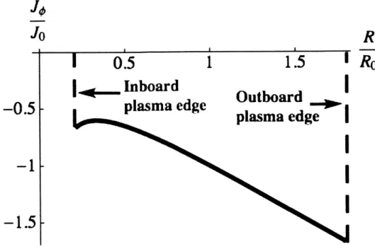
Unfortunately, the Solov'ev profiles (1.4) correspond to a somewhat unrealistic

situation from an experimental point of view, since the toroidal current density has a

jump at the plasma edge. For this reason, we demonstrate in the remainder of

Chapter 2 that the procedure we developed for the Solov'ev profiles can be applied as

successfully for more realistic profiles, given by:

In (1.5), B is the vacuum magnetic field, a represents the plasma diamagnetism (a > 0) or paramagnetism (a < 0), and p, is defined such that the pressure at the

magnetic axis is Paxis = P₀ as

The solution of the GS equation which we find for the profiles (1.5) is more

complicated than in the Solov'ev case. Instead of a polynomial expansion, we now

have an expansion in Whittaker functions. Most importantly, some of the

undetermined constants now appear nonlinearly in the solution, namely in the

argument of Whittaker functions. However, the procedure to determine the free

constants which we presented in the Solov'ev case can be applied in exactly the same

way. The only difference is that the system of algebraic equations for the boundary

constraints is now nonlinear. Solving this system is a less trivial numerical problem

than in the previous case, and convergence issues may be encountered if the chosen

geometric and plasma parameters are too extreme. Nevertheless, in most cases the

system can readily be solved by calling a built-in nonlinear solver in any scientific

computing program. We have been able to compute very plausible tokamak and ST

equilibria with this procedure, for a wide range of parameters, and with or without

Part 2: MHD comparison theorems, and the vanishing of plasma

compressibility

One of the most important criteria in the design of a magnetic fusion

experiment is the stability of the plasma to the fast macroscopic modes known as

MHD modes. These modes are known experimentally to considerably degrade the

plasma properties, and can actually cause the termination of the plasma discharge.

MHD instabilities are usually studied using the ideal MHD model, because of

the relative simplicity of this model, and of its particular mathematical properties. In

ideal MHD, the problem of linear stability in any 3D configuration can be cast in a

very convenient form known as the ideal MHD energy principle. It can be stated as

follows:

A static ideal MHD equilibrium is stable if and only if

6WMHD >0 (1.6)

for all allowable displacements (.

In eq. (1.6), ( is the plasma displacement, and 6W(*,

)

associated with the displacement (. The energy principle (1.6) can be refined, and a

e In ergodic systems (tokamaks, stellarators, STs, etc.), or closed field line

systems with modes which do not conserve the closed-line symmetry, a static ideal MHD equilibrium is linearly stable if and only if

_W

* 0 (1.7)

for all allowable displacements .

In eq. (1.7), 8W (* ,() is the potential energy associated with incompressible

displacements. In other words, ideal MHD stability, for this first family of

modes and magnetic geometries, in inherently incompressible.

* For closed field line systems (Z-pinch, Dipole, FRC, etc.), and modes which

conserve the closed-line symmetry, a static ideal MHD equilibrium is linearly stable if and only if

6W *= SW+( *,) + f p (V.- )}2 dr 0 (1.8)

for all allowable displacements .

In eq. (1.8), ( ) represents the flux-tube averaging operation. 6W , the

compressible piece of 6WMHD

(

the previous case. Since it is clear that 6W

(*,

)

stabilization. Some closed field line devices, such as the Levitated Dipole

eXperiment (LDX), rely explicitly on MHD compressibility to stabilize their

most dangerous MHD modes.

The ideal MHD model relies on the assumption that both the electrons and the

ions are collisional on the MHD time scale. In this approximation, the plasma is

isotropic, and kinetic effects are absent. In most modern magnetic confinement

experiments and in future fusion reactors, this assumption is not justified, at least for

the ions. Fusion grade plasmas behave in a fundamentally anisotropic manner, and

kinetic effects are ubiquitous. One can therefore wonder how robust the ideal MHD

stability analyses and the ideal MHD energy principle are in plasmas of fusion

interest. For example, a question of interest for closed line systems such as the LDX

is the reliability of the criterion (1.8). The factor y in 6W comes from the ideal

MHD equation of state d

/

/

that the plasma behaves as an isotropic fluid, one may have doubts about the

robustness of (1.8), and about the existence of MHD compressibility stabilization.

In Chapter 3 of this thesis, we assess the reliability of the ideal MHD energy

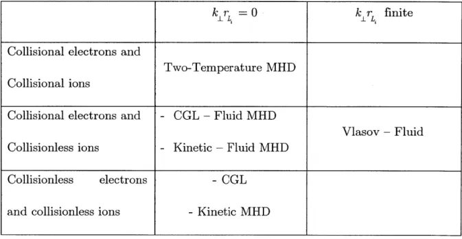
principles for both ergodic and closed line systems. We introduce six models which

extensively. They are presented in Table 1, in which they are organized according to

the collisionality regime they are associated with, and to whether or not they allow

for finite krL , where k, is the perpendicular wave number of the modes of interest,

and rL is the ion Larmor radius.

kL r = 0 k r finite

Collisional electrons and

Two-Temperature MHD Collisional ions

Collisional electrons and - CGL - Fluid MHD

Vlasov - Fluid Collisionless ions - Kinetic - Fluid MHD

Collisionless electrons - CGL

and collisionless ions - Kinetic MHD

Table 1.1 The six models which are compared to the ideal MHD model

For each of the models shown in Table 1, we derive new expressions for the

potential energy of the plasma displacement, and new quadratic energy relations,

valid in arbitrary 3-D configuration, which we compare with 6WMHD and with the

The stability boundaries predicted by ideal MHD are more conservative than

those predicted by any of the models in Table 1.1 assuming krL = _{0. In other words,}

ideal MHD linear stability implies linear stability in any of these models. The

situation is different, however, when ideal MHD is compared with the Vlasov-Fluid

(VF) model, a model which is constructed specifically to allow finite k₁ rL , and which

assumes that the equilibrium ion distribution function depends only on the total

energy (so that there is no equilibrium ion flow, as in ideal MHD). Indeed, in this

thesis we prove the following statement:

For both ergodic and closed line magnetic geometries, the condition for the marginal stability in the VF model is:

6W ₁ = 0 (1.9)

Two important consequences can be deduced from (1.9). First, note that for

ergodic systems, the condition (1.9) is identical to the condition (1.7). In other words, for ergodic systems, the ideal MHD energy principle for incompressible displacements

accurately predicts the linear stability boundaries. It is not a conservative estimate

as has been thought in the past, but corresponds to the actual stability boundary.

Second, plasma compressibility is absent from the criterion (1.9). Thus, according to the VF model, in closed line systems, the linear stability boundaries

determined with the ideal MHD model are not the most conservative. A plasma can VF unstable to an MHD mode, and yet found to be ideal MHD stable.

Physically, we find that for the equilibria under consideration in the VF

model, in which the ions are electrostatically confined, kinetic effects associated with

the drift of the particles perpendicular to the magnetic field lines are responsible for

the vanishing of plasma compressibility. Of all the models shown in Table 1, only the

VF model can treat resonant particle effects perpendicular to the field lines. In fluid

models, kinetic effects are obviously absent, and in the other kinetic models, which

assume rL = 0, particles do not drift off the flux tubes they are attached to. This

explains why the result given in (1.9) is new. Until now, there was a shared belief,

supported by a large number of studies with the CGL and Kinetic MHD models, that

ideal MHD stability boundaries were always the most conservative, both in ergodic

and closed line systems.

Our new result may be most important for closed line configurations, such as

the levitated dipole and the FRC, where MHD compressibility stabilization plays an

important role in predicted plasma performance. Therefore, in Chapter 4 we illustrate

its implications by studying the case of the hard-core Z-pinch, a closed line

configuration which is the large aspect ratio limit of the levitated dipole.

Ideal MHD stability theory shows that in a hard-core Z-pinch, the most

unstable mode is the compressible interchange mode. This mode is driven unstable by

small enough pressure gradients, the mode is stabilized by plasma compressibility. In

low 3 plasmas, the condition on the pressure gradient is

r dp '

< 2-= 10 / 3 for ideal MHD stability (1.10)

p dr

Based on our analysis in the previous section, we expect this condition to be

violated in the VF model, and the instability to persist beyond the ideal MHD

stability limit, once resonant particle effects perpendicular to the field lines are taken

into account. Therefore, we derive the eigenvalue equation for the interchange mode

in the VF model, and solve this equation numerically. The VF criterion for stability

we obtain from our numerical analysis is the following:

r dp

< 0 for Vlasov-fluid stability (1.11)

p dr

Eq. (1.11) proves the absence of plasma compressibility stabilization in the VF model, which applies to the particular class of hard-core Z-pinch equilibria in which

the ions are electrostatically confined. Thus, when ion kinetic effects perpendicular to

the field lines are included, the instability persists beyond the ideal MHD limit, and

only non-decaying pressure profiles are linearly stable. Such profiles are obviously not

desirable for magnetic fusion concepts.

When k r _{is small, the growth rate of the instability is small in the ideal}

MHD stable regime. This is expected, since the instability is only due to a few

becomes larger as k, gets larger, and may be comparable to ideal MHD growth rates

when kr ~1.

Additionally, our VF numerical studies show that to fully account for the

resonant ion effects, it is crucial to solve the full eigenvalue equation. Often, this

equation is simplified by assuming that the mode has scale lengths which are much

shorter than those of the equilibrium quantities. This is the so-called local

approximation. However, the results we obtain in this approximation are

qualitatively different from the results we obtain solving the global eigenvalue

equation, even when the approximation is justified. The reasons for this discrepancy

are two-folds: 1) The details of the profiles (pressure, magnetic field) explicitly appear

in the resonant denominators; 2) The real frequency of the mode given by the global

eigenvalue equation is different from the one obtained by solving the equation at a

given location, which modifies the resonance condition.

We conclude this thesis by discussing the experimental relevance of the VF

results, and by suggesting ways to verify the robustness of these results with models

Chapter 2

Static MHD equilibria and analytic solutions to the

Grad-Shafranov equation

We focus, in this chapter, on one aspect of ideal MHD equilibrium theory,

namely the calculation of analytic self-consistent MHD equilibria. What exactly do

we mean by analytic equilibria? We will show in the first part of this chapter that for

toroidally axisymmetric confinement concepts (i.e. almost all the magnetic

confinement machines which show promise as future fusion reactors, except for the

notable exception of the stellarator), the equation describing the equilibrium of the

plasma can be cast in the form of a two-dimensional, nonlinear, elliptic partial

differential equation called the Grad-Shafranov equation (GS equation). The solution

of the GS equation, with its associated boundary conditions, fully determines the

equilibrium. (Section 2.1). In general, the GS equation has to be solved numerically

[1]. However, for particular, somewhat idealized equilibrium pressure and current profiles, analytic solutions to the GS equation can be obtained. This is what we mean

point of view: we can use them to develop our intuition about a particular

confinement concept, to perform analytic calculations of the stability and transport

properties of that concept, or to benchmark numerical solvers of the GS equation.

Our new analytic solutions to the GS equation are presented in the second and

third parts of this chapter. We first present new analytic solutions of the GS equation

for the pressure and current profiles known as Solov'ev profiles [2], simple profiles which still retain most of the crucial physics involved in the theory of MHD equilibria

in toroidally axisymmetric devices. The attractiveness of the solutions we propose lies

in their simplicity, and versatility. Indeed, we show that by using a single,

streamlined procedure, these solutions can be used to calculate MHD equilibria of

tokamaks, spherical tokamaks (STs), spheromaks and field reversed configurations

(FRCs), and we give examples for each configuration. (Section 2.2)

The difficulty with the Solov'ev profiles is that they are partially unrealistic

experimentally, since they correspond to a situation where the pressure gradient and

the current profiles have a jump at the plasma edge. The purpose of the third part of

this chapter is to demonstrate that the procedure described in Section 2.2 can in fact

be generalized to more realistic profiles. We find analytic solutions to the GS

equation for profiles characterized by the vanishing of the pressure gradient and of

the current at the plasma surface. These analytic solutions have the same number of

degrees of freedom as the ones we propose in the Solov'ev case, so that the

With these solutions, we calculate tokamak and ST equilibria, with and without

up-down symmetry.

2.1 Confined plasma equilibrium and Grad-Shafranov equation

2.1.1 Equilibrium equations in fusion plasmas

We start with the ideal MHD momentum equation:

dv

p =_ JxB-Vp

dt (2.1)

An equilibrium is defined by the fact that all the quantities involved in eq. (2.1) are

time-independent, - = 0. In these conditions, eq. (2.1) becomes

at

pv- Vv J x B - Vp (2.2)

Furthermore, comparing the inertial term and the pressure gradient term, we have

the following scaling:

pv.-Vv _{~ ~l -}v2 _{- m2}2

Vp v T2 (2.3)

where we have assumed that the ion and electron temperatures are comparable (a

very good assumption in fusion grade plasmas), and where we have introduced the

ion Mach number Mi as the ratio of the plasma velocity to the ion thermal velocity.

In toroidally axisymmetric geometries, one usually distinguishes the poloidal velocity,

the plane perpendicular to the axis of symmetry. Consequently, one often separates

the poloidal Mach number M, and the toroidal Mach number, MT. In magnetic

fusion experiments, we typically have M, < M T (e.g. [3]), so that the ordering in

(2.3), and the question of keeping or neglecting the inertial term in eq. (2.2)

essentially depends on MT.

In the absence of external momentum input, in particular from neutral beam

injection systems, the upper bound MT < 0.15 is usually found in modern fusion

experiments (e.g. [4] for the DIII-D tokamak [5] and [6] in the Alcator C-Mod

tokamak [7]), so that the inequality M2

_<1

auxiliary torque input, through neutral beams for instance, as in the DIII-D tokamak

and the NSTX spherical tokamak (ST) [8], the plasma flows can be larger. Still, the

values typically observed are of the order MT, 0.5 ([9], [10]), so that the ordering

M, < 1 is still somewhat acceptable. It will most likely be even more acceptable in

the ITER tokamak [11], where the momentum input from the neutral beam system is

expected to be smaller, because of the large machine size, and the higher densities.

In conclusion, we can say that for almost all situations of fusion interest,

neglecting the inertial term is justified, and we can focus on static equilibria, v = 0,

for which the equilibrium momentum equation takes the form:

(2.4) J xB = Vp

which is the well-known equation expressing the balance between the magnetic force

J x B and the pressure gradient force.

The three components of Eq. (2.4) represent three equations for seven unknowns:

p, the three components of J and the three components of B. This is obviously not sufficient to fully determine the equilibrium. The remaining equations are obtained

from the low-frequency version of Maxwell's equations, consistent with the ideal

MHD ordering: V -B = 0, and V x B = ptJ. Thus, ideal MHD equilibria are

calculated from the following system of equations

V -B = 0

V x B =btpJ (2.5)

J x B Vp

and we now indeed have seven equations for seven unknown, so that the problem is

well-posed. In Section 2.1.2, we show that for toroidally axisymmetric plasmas, all the

information contained in the seven equations given by eq. (2.5) can be expressed in a

single equation for one variable: the Grad-Shafranov equation. This is our next task.

Before doing so, however, it is worth mentioning that although we derived eq.

(2.5) from the set of equations defining the ideal MHD model, and although the computation of plasma equilibria in magnetic confinement concepts is usually

considered a part of ideal MHD theory, the equilibrium described by eq. (2.5) is in

fact consistent with descriptions of the plasma which are more accurate than ideal

MHD, and valid in regimes where ideal MHD is not, in particular in regimes of fusion

interest, where the plasma ions are collisionless (cf. Chapter 3). This is shown as

follows.

First, V -B = 0 and V x B = ptJ are the equations of magnetostatics, the

steady-state version of Maxwell's equations for the magnetic field. They are obviously

exact equations when -= 0, independently from any consideration about the

1t

collisionality of the plasma.

The discussion about the momentum equation is more subtle. Taking the

exact second order moment of the electrons' and ions' Maxwell-Boltzmann equations,

and adding them, we obtain the exacti momentum equation for the whole plasma:

dv

p-+V -(H + 1) J x B- Vp (2.6)

dt

For the same reasons as the ones previously presented, we can neglect the inertial

term in eq. (2.6): - 0 in steady-state, and for flows which are subsonic. We also

dt

know that the viscosity tensors H and H, vanish identically if the ion and electron_Ze

to be more precise, we made an assumption to obtain eq. (2.6), namely that the electron inertia is negligible compared to the ion inertia, so that the plasma inertia can be identified to the ion inertia.

equilibrium distribution functions are exact Maxwell-Boltzmann distributions. The

question about the validity of eq. (2.5) in collisionality regimes of fusion interest is

then the following: what is the condition on the ion and electron collisionality for the

distribution functions to be Maxwellian in equilibrium? In particular, can we assume

that the ions are in thermal equilibrium (i.e. are well-represented by a

Maxwell-Boltzmann distribution) when we know that ions are essentially collisionless in fusion

grade plasmas?

The answer, perhaps surprisingly, is yes. The main reason is that, by

definition, equilibrium equations describe the steady-state behavior of the plasma, or,

in other words, its evolution on very long time scales. And on these long time scales,

even weak collisions eventually Maxwellianize the plasma, and drive it towards

thermal equilibrium [12]. Using an entropy production argument, it can be shown [13]

that the condition for the ion and electron distribution functions to be Maxwellian to

lowest order only relies on the fact that in magnetic confinement systems, the

particles' Larmor radius is much smaller than the typical macroscopic size of the

system. In fusion grade plasmas we therefore have H - 0, H, ~ 0 in equilibrium, and

J x B ~ Vp.

The bottom line of all this discussion is that eq. (2.5) is valid far beyond the

limits of ideal MHD, and in particular reliably represents equilibria of fusion grade

plasmas, at least when neutral beam heating and current drive systems are turned

2.1.2 Equilibrium in toroidally axisymmetric plasmas: the Grad-Shafranov equation

As announced in the previous section, we now show how the set of seven

equations for seven unknowns given in (2.5) reduces, for toroidally axisymmetric

configuration, to a single two-dimensional, nonlinear, elliptic partial differential

equation, whose solution contains all the information necessary to fully determine the

nature of the equilibrium. This was first discovered by Lnst and Schlniter, Grad and

Rubin, and Shafranov in the years 1957 to 1959 [14], [15], [16]. In this section, we

rederive this equation, now known as the Grad-Shafranov equation (GS equation),

following the presentation given in [17].

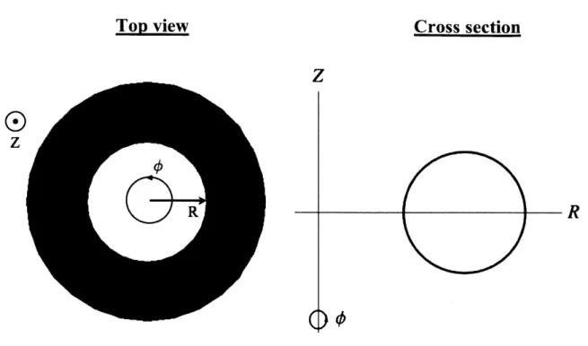
For toroidally axisymmetric geometries, the natural coordinates are the (R,#,Z)

cylindrical coordinates, where

#

with circular cross section.

We start with the first equation in (2.5): V -B - 0. Of course, because of the

toroidal axisymmetry, this equation does not give us any information about B,, the

#

Cross section

Z

0

z

R

Fig. 2.1. Geometry for toroidally axisymmetric equilibria and cylindrical coordinates

which is the field in the (R, Z) plane. Indeed, V -B = 0 implies that B can be

written as B = V x A , where A is the vector potential. And with the axisymmetry,

only A, appears in the expressions for BR and Bz

B-

-R&Z R OZ

1 a(RA)

z R OR (2.7)

As is often done in fluid dynamics, it is then very convenient to introduce a stream

function T , defined by T = RA, , to write

1

B =- Be

+

where e. is the unit vector in the

#

The physical interpretation of the stream function T is straightforward: it is the

poloidal flux TP normalized by dividing by a factor 27. This is shown as follows.

The poloidal flux is defined by T, = f B, -dS, where dS is an infinitesimal surface

element. If we choose to calculate the poloidal flux through the area of a washer

shaped surface in the plane Z = 0, extending from the magnetic axis, located at

R = Ra, to an arbitrary T contour, at R = Rb, we find:

2 Rb 2r

1

a

As we can see from eq. (2.7), P is defined to within an arbitrary integration

constant. Choosing this arbitrary constant so that (R,0) 02, eq. (2.9) becomes:

T, = 27w (2.10)

which proves our statement.

The next step in the derivation of the GS equation is to use the low-frequency

version of Ampere's law, V x B= pJ, to obtain an expression of J in terms of the

stream function IV. Ampere's law is formally identical to the equation linking the

magnetic field and the vector potential, so that we immediately obtain, for the

poloidal current,

2 _{Note that we will choose the arbitrary constant in a different way in Section 2.2,} where it will be more convenient to choose it such that T = 0 on the plasma surface

poJp = - V (RB,) x e,

The toroidal current is

BR B tiJaz OR

1

'rl04''

where, as usually done in MHD equilibrium theory, we have introduced the elliptic

operator A- _{, given by} A*X = R2V. ] R 2, (2.13) R I1 OX' 2X R -- - +_ OR R OR, OZ2

We are now ready for the last three steps in the derivation of the GS equation, which

consists in projecting the momentum equation J x B = Vp onto the three vectors B,

J, and VTI.

0 Projection onto B

It is clear that the left-hand side of the momentum equation is orthogonal to B.

Because of the axisymmetry, Vp has only R and Z components, so that the

result of the projection is

e,).Vp = 0 e, -VWxVp = 0 (2.14)

Now, VT x Vp only has a

#

VT x Vp = 0Op = p

(WV)

(VW

x

p depends on T only, it is a surface quantity. Projection onto J

From the formal equivalence of the role played by B and J in the momentum

equation, it is clear that the projection onto J leads to the following equation:

.Vp=

* e, -V(RB )xVW = 0

In the second line of eq. (2.16), we used the fact that p = p(A) . We now are in the same situation as in eq. (2.14), and in the same way, we conclude that

RB, = F

(T)

The quantity RB, depends on I' only, and is a surface quantity like p. As with

T , there is a physical interpretation for the quantity F: it is the net poloidal

current flowing in the plasma and the toroidal field coils normalized by dividing

by a factor -27r. To prove this, we calculate the flux of the poloidal current

density through a disk-shaped surface lying in the Z = 0 plane, extending from

R = 0 to an arbitrary 4 contour at R = R6. We find:

27r

I, = f J, -dS -J d# dRRJz

0 0

(R,

Z

which proves our point. In (2.18), the

0 0

sign comes from the fact that the element

of surface dS is oriented in the

+Z

0 Projection onto VP 1 _R (2.16) 27r =-wFOF =.0) =f d#f dR = - -27rF(T) (2.18)

We are now ready to calculate J x B = (J e + J x (Be, + B).

product between the two toroidal components obviously vanishes. Furthermore,

J x B = 0 since VT x e, -e, = 0 , and VT x e -VT = 0. Therefore, the only contributions come from the cross terms between poloidal and toroidal

components.

calculate that

Using the so-called "BAC-CAB" vector identity, it is easily to

J J 0e 0x B =LL VT -R 1 J xBe =- F p 40 1 1 _A*qfVq (2.19) dFV

_Vi

For toroidally axisymmetric geometries, the momentum equation can therefore be

written as 1 A* - AIVp pu0R2 1_ dF -oRV2 d (2.20) dp d T

We see here that the only non trivial information in the equilibrium force balance

equation is contained in the VT component, as expected. Eq. (2.20) is usually

written in the form

A*ip = --poR2

-P- F F (2.21)

This second-order, nonlinear, elliptic partial differential equation is the Grad

Shafranov equation (GS equation). Once the two free functions p and F are chosen, The cross

and the boundary conditions fixed, the GS equation can be solved, and the solution

T fully determines the nature of the equilibrium. In the next two sections (Sections

2.2 and 2.3), we focus on particular profiles for p and F, profiles for which we will

be able to find analytic solutions to the GS equation.

2.2 Analytic solutions of the Grad-Shafranov equation with

Solov'ev profiles

2.2.1 Analytic solutions of the Grad-Shafranov equation

In general, the GS equation has to be solved numerically, and since the late

1950s and the first derivation of the equation, several excellent accurate and fast

numerical Grad-Shafranov solvers have been proposed (see for instance [18] and

references therein). Nevertheless, analytic solutions are always desirable from a

theoretical point of view. They usually give more insights into the properties of a

given equilibrium than numerical solvers do, for instance when used to derive scalings

with the different geometric parameters (aspect ratio, elongation, triangularity). They

can also be the basis of analytic stability and transport calculations. Finally, they can

be used to test the numerical solvers.

In several confinement concepts of fusion interest, such as the tokamak and

the stellarator for instance, the inverse aspect ratio is a small number which can be

used as an expansion parameter in eq. (2.21). Analytic solutions are obtained by

3 _{A significant portion of Section 2.2 can be found in A.J. Cerfon and J.P. Freidberg,} Phys. Plasmas 17, 032502 (2010).

expanding (2.21) order by order, as one usually does in asymptotic calculations. This

method has led to a wealth of results, and a very deep analytic understanding of

static equilibrium in tokamaks (See for instance [17] and [19]).

The problem, of course, is that asymptotic expansions break down in other

confinement concepts of fusion interest, such as spherical tokamaks (STs),

spheromaks, or Field Reverse Configurations (FRCs), in which the inverse aspect

ratio is close to 1. In this case, of course, analytic solutions can only be found for

specific, cleverly chosen profiles for the functions p and F. In 1968, Solov'ev [2]

proposed simple pressure and poloidal current profiles which convert the GS equation

into a linear, inhomogeneous partial differential equation, much simpler to solve

analytically. Despite their simplicity, and the fact that the current density is finite,

not zero, at the plasma edge, these profiles still retain much of the crucial physics

that describes each configuration of interest, and have, therefore, been extensively

studied, particularly for spherical tokamaks [17], [20], [21], [22]. The analytic solutions

of the GS equation investigated in these papers have been used in the study of

plasma shaping effects on equilibrium [23] and transport [24], [25] properties.

A general property of these analytic solutions is that they contain only a very few terms, thereby making them attractive from a theoretical analysis point of view.

One down side is that while the solutions exactly satisfy the GS equation, one is not

free to specify a desired shape for the plasma surface on which to impose boundary

optimizing over the small number of terms kept in the solution. Specifically, this

mini-optimization results in limits on the class of equilibria that can be accurately

described. For instance, reference [17] focuses solely on low-0 equilibria, where the

toroidal field is a vacuum field. It thus cannot describe the equilibrium

3

#

triangularities. It is ill behaved for moderate to large triangularities. In references [21]

and [22], the solutions allow for an inboard separatrix for a wider range of

triangularities, but appear to be over constrained in that the shape of the plasma

(elongation and triangularity) depends on the choice of the location of the poloidal

field null. Often trial and error is required to choose certain free coefficients that

appear in the optimization in order to obtain an equilibrium with certain desired

qualitative properties. Rarely, if ever, are non-tokamak configurations considered.

The goal of this section and of this chapter as a whole is to present a new,

extended analytic solution to the GS equation with Solov'ev profiles which possesses

sufficient freedom to describe a variety of magnetic configurations: the standard

tokamak, the spherical tokamak, the spheromak, and the field reversed configuration.

This new solution possesses a finite number of terms but includes several additional

terms not contained in previous analyses. Our solution is valid for arbitrary aspect

ratio, elongation, and triangularity. It is also allows a wide range of 3: (1)

#

that could have the value zero, and (3) high 3 equilibria where a separatrix moves

onto the inner plasma surface. Lastly, the solution allows the plasma surface to be

either smooth or to possess a double or single null divertor X-point. Most

importantly, no trial and error hunting is required. A simple, direct, non-iterative,

one-pass methodology always yields the desired equilibrium solution.

In the remainder of this section, we describe how to derive the new extended

solution (section 2.2.2), explain the procedure we use to systematically calculate the

free coefficients in our solution (section 2.2.3), and use the solution to calculate

equilibria and figures of merit in all the geometries of interest and for all the beta

regimes mentioned previously (section 2.2.4 to section 2.2.9).

2.2.2 The Grad-Shafranov equation with Solov'ev profiles

The GS equation (eq. (2.21)) can be put in a non-dimensional form through

the normalization R = Rox , Z = Roy, and I = Too, where Ro is the major radius of

the plasma, and Weis an arbitrary constant:

8 0p 2p R14 dp Res dF

x+ -o R _F (2.22)

Ox x

Ox,

00

The choices for p and F corresponding to the Solov'ev profiles are given by

[2]

R dp

"P q12 _dop

2 0 (2.23)

R2 dF

where A and C are constants. Since To is an arbitrary constant, one can, without

loss in generality, choose it such that A

+

rescaling To' -- (A + C)T'. Under these conditions, the GS equation with Solov'ev

profiles can be written in the following dimensionless form

a

x 1±

+

Dx z\ Dz y2

The choice of A defines the

= (1 - A)x 2

+ A

#

consideration. In the following sections, we will calculate equilibria in various

magnetic geometries for particular values of A corresponding to a range of 3 values.

The solution to eq. (2.24) is of the form

_(x,y)

is the particular solution and @b is the homogeneous solution. The particular

solution can be written as

4

8 A -X2 Inx- -4

2 8

(2.25)

The homogeneous solution satisfies

z- - VH + H

aX X (9X ,

y2

4 The special case A + C = 0 cannot occur for physical equilibria since it corresponds to a situation beyond the equilibrium limit where the separatrix moves onto the inner

plasma surface.

(2.24)

A general arbitrary degree polynomial-like solution to this equation for plasmas with up-down symmetry has been derived by Zheng et. al. in [20]. We

present here the details of this derivation.

Given the form of eq. (2.26), and the fact that we look for solutions which are

even in the variable y (up-down symmetry), we assume that there exists a general

solution of the form of the expansion

n/2

OH (XIY)

>Z

n=0,2,... k=0

where, the expansion can stop at any desired n, and where G is a function which is

not yet determined, but which we expect to have a similar form as the particular

solution @,, namely either a power of x, or a power of x multiplying ln x. Now, if

(2.27) is a solution, it obviously has to satisfy the equation (2.26). Inserting (2.27) into (2.26), and identifying the terms where y has the same exponents for a given n,

we obtain the following recurrence relations on the index k, for a given n:

,_ 1 1B0G(n, 0,x)=0

(2.28)

Xn-2k.1)n-2k+2 G(n,k -1,x) k - 0

As can be seen by focusing for instance on the case k = 0, there are two types

of solutions to eq. (2.28) (In the case k =0, they are G1(n, 0, x) =1 and

G2(n,0,x)= x2). Thus, we write

G(n, k, x) c1G

(n,

(n,

where the cni and c2 are free constants. With a proof by induction, it is then easy to

show that if G1 and G2 take the following general forms:

G1(n,0,x) = 1

G1(I,k> 0,z)

(-1)k

(n - 2k) ! 22 k!(k - 1)! k

j

G2(n,k, z) =

(-

(n - 2k ! 22'k! !(k + 1)!

they satisfy the recurrence relation (2.28), so that the solution assumed in (2.27) does

indeed solve the differential equation (2.26).

The solutions given by the form in GI are what we call the polynomial-like

solutions (since they involve ln x), while the solutions obtained from G2 are

obviously the polynomial solutions. Eq. (2.30) is extremely convenient, since we can

use it to calculate solutions to the GS equation with Solov'ev profiles in the form of

polynomials (and polynomial-like terms) of arbitrary degree. For our purposes we

need only a finite number of terms in the possible infinite sum of polynomials and

polynomial-like terms. We truncate the series such that the highest degree

R 4 and Z4. The full solution for up-down symmetric V) including the most general

polynomial and polynomial-like solution for 'bH satisfying eq. (2.26) and consistent

with our truncation criterion is given by

4

'

1

(X,

+

+]cii

9)

8y6 _{- 140y}4_x2

₊

₊

Equation (2.31) is the desired exact solution to the G-S equation

describes all the configurations of interest that possess up-down symmetry. (2.31)

that

The

unknown constants c are determined from as yet unspecified boundary constraints

on 0. We note that the formulation can be extended to configurations which are

up-down asymmetric. This formulation is described in Section 2.2.9. However, for

simplicity the immediate discussion and examples are focused on the up-down

symmetric case. Thus, our next task is to determine the unknown c appearing in eq.

2.2.3 The boundary constraints

Assume for the moment that the constant A is specified (we show shortly how

to choose A for various configurations). There are then seven unknown c to be

determined. Note that, as stated, with a finite number of free constants it is not

possible to specify the entire continuous shape of the desired plasma boundary. This

would require an infinite number of free constants. We can only match seven

properties of the surface since that is the number of free constants available.

Consider first the case where the plasma surface is smooth. A good choice for

these properties is to match the function and its first and second derivative at three

test points: the inner equatorial point, the outer equatorial point, and the high point

(see Fig. 2.2 for the geometry). While this might appear to require nine free constants (i.e. three conditions at each of the three points), two are redundant because of the

up-down symmetry.

Although it is intuitively clear how to specify the function and its first

derivative at each test point, the choice for the second derivative is less obvious. To

specify the second derivatives we make use of a well-known analytic model for a

smooth, elongated, "D" shaped cross section, which accurately describes all the

configurations of interest [26]. The boundary of this cross-section is given by the

parametric equations

X = 1+ Ecos(T+ asinT) _(2.32)

where T is a parameter covering the range 0< T

<

/

inverse aspect ratio, K is the elongation, and sin a = 6 is the triangularity. These

three parameters have been geometrically defined in Fig. 2.2. For convex plasma

surfaces the triangularity is limited to the range 6 <sin(1) ~ 0.841. The idea is

simple: we match the curvature of the plasma surface determined by our solution

with the curvature of the model surface (2.32) at each test point. We now show how

this is done in practice.

R/R0

Fig. 2.2. Geometry of the problem and definition of the normalized geometric

parameters E, tK, and 6 High point Outer equatorial point Inner equatorial point