Cascade performance with accelerated or decelerated axial velocity

kk, "'A',

ACCELERATED OR DECELERATED AXIAL VELOCITY

by SHIGEO KUBOTA

Under the sponsorship of:

General Electric Company

Allison Division of General Motors Corporation

Westinghouse Electric Corporation

Gas Turbine Laboratory

Report Number 56 September

1959

ABSTRACT

ACKNOWLEDGEMENTS

1. INTRODUCTION

2. FLAT PLATE CASCADE 3

3. CASCADE COMPOSED OF ARBITRARILY SHAPED BLADES 18

4. CORRECTION FOR SECONDARY FLOW 24

5. NUMERICAL EXAMPLES 25

6. CONCLUSIONS 26

A theoretical method to estimate the effect of axial velocity change through a cascade was investigated. The change of axial velocity was reproduced by distributing sinks and sources within the blade

pas-sages, and the conclusions are set forth in some simple formulae. Some graphs for the numerical evaluation of the performance of NACA 65 eries cascades were prepared, and several examples were compared with experi-mental data.

This report is the realt of an investigation, which was per-formed during my stay at the Gas Turbine Laboratory for several months. During this period, I was treated quite the same as the other staff mem-bers and spent a most profitable and pleasant time. I should like to thank all the members of the Gas Turbine Laboratory, particularly Pro-fessors E. S. Taylor and Y. Senoo who always gave me the most useful ad-vice and encouragement. Professor S. Otsuka of Nagoya University, Japan, sent me a useful report and valuable Advice for which I am most thankful. I must express many thanks to Mr. J. Brown who assisted me most effectively in the preparation of the manuscript. The skillful typewrit-ing is due to the efforts of Vrs. N. Appleton.

My stay at this laboratory would not have been possible without the financial support of my company, Kawasaki Dockyard Co., Kobe, Japan;

The study of cascade performance, as a result of a changing axial velocity within the blade passages, is important in the design of axial flow turbomachinery. In most of the multi-stage axial flow compressors and turbines, the magnitude of axial velocity varies considerably from the first to the last stage, because of the design requirements. Small

axial velocity changes accumulate from each stage. Therefore, it is somewhat inexact to use the experimental data of cascade tests which are obtained under the condition of constant axial velocity, without any cor-rection.

There is another reason why this problem is important. In the usual cascade wind tunnel test, owing to the development of a boundary layer on the surface of the side wall of the cascade, the axial velocity in-creases at the midspan through the cascade. In order to keep the axial velocity constant, the boundary layer must be sucked off in some way, making the experimental technique more time consuming. Therefore, if the experimental data without any boundary layer remov&l can be cor-rected to the case of constant axial velocity, there is a certain pos-sibility of reducing the difficulty of cascade testing very much.

N. Ztholz (1), S. Katzoff (2) and W. R. Hawthorne (3) wanted to solve this problem and devised some equations to correct such an effect. How-ever, since their treatment was based on a simple one-dimensional con-sideration, it seems to be insufficient to explain such a pomplicated

phenomenon. J. R. Erwin and J. C. Emery (4) proposed three empirical methods to cozrect the turning angle but, as the authors themselves said

they didn't cover any of the experimental evidence. Later, T. Kawasaki (5) carried out a method based on the two-dimensional treatment. In his method, he put a concentrated source at the middle point of the blade passage cor-responding to the increment of the axial velocity. However, there is some

doubt whether or not it is proper to express the effect of the axial ve-locity increment by such a concentrated singularity. The method here de-veloped is based on the idea that sources are distributed in the whole

doain of the blade passage, corresponding to the increase or decrease of the axial velocity. This assumption seems to be a more accurate

expres-sion of the phenomenon.

Generally speaking, there are many factors which would be related to the change of axial velocity. They are; hub ratios at the inlet and exit of the stages, accumulation of boundary layer thickness through stages, ef-fect of compressibility, effect of secondary flow and leakage or extraction at any stage. In most cases, one might consider that all of these effects appear separately. The method here described can cover all of the effects mentioned above, except the effect of compressibility and secondary flow.

The correction regarding these two factors must be taken into account in a proper way, if it is necessary.

2. FLAT PLATE CASCADES

First consider a most simplified cascade, that is, the cascade com-posed of flat plates. In this theoretical consideration the following basic assumptions are presupposed; flow is steady, two-dimensional, non-viscous and incompressible.

d

_____

0j

C

x010

- 1j

~

I

1 -

---The cascade to be considered is composed of flat plates, whose chord length is c, spacing is s, stagger angle is ' . At the inlet of the

cascade flow is quite uniform, and its direction is changed by the cas-cade, flowing off to the right. In the cascade, from 0 C3i to

C , the axial velocity of the flow is accelerated (or in-versely, decelerated) from val to va2.

In such a case our problem is to determine the performance of the

cascade. That is, given the values of mean velocity direction measured from the chord line a, the magnitude v, and the changing condition of axial

j

% q

ef

;7--,

velocity within the blade passage

A

(Q),

calculate the value of the circulation around a blade

r

as a function of

1

=.S/c

,'(V

and . In this paper, variations of axial velocity were treated

as a function of t only, and independent of

7

.

To solve this problem, we divide the flow into three elementary parts: (i) Flow around the given cascade with a given mean velocity

vector, without any change of axial velocity.

(ii) Flow consisting of a source and sink distribution only, corresponding to the given axial velocity change (the boundary condition is not satisfied).

(iii) Flow to cancel the normal velocities on the blade sur-face which were induced by the flow (ii), and an

ad-ditional circulation to satisfy the Kutta-Joukowski's condition at trailing edge₉

By superimposing the three elementary flows above, we can obtain the flow which satisfies all the prescribed conditions.

2 - 1. Flow (i)

The solution of Flow (i) is already well known, and in this paper the conclusive equation only shall be given,

4

KS---where,

)(

is a parameter depending upon the values of the blade pitch-chord ratio

7\

, and the stagger angle I . Although the functional

relation )C =

f

(A, -) is rather complicated, we can easily find it in the numerical tables (6).

2 - 2. Flow (ii) '- ,~ %

CCa

a I '

O

*1 2 2 -7

Next the relation between the source or sink distribution and the varia-tion of axial velocity must be examined. Consider the source distribution

spread over the belt-wise domain from E C.4 to : C4S

The strength of source per unit area is expressed by , and it is a

func-tion of 5 only.

Velocity induced at an arbitrary point ( e ,j ) by this source distribution can be easily calculated by the law of Biot Savart, and is written as follows,

.

SS

7o

Z

Coos

where

(

)

(1_10)t

Equation (2) can be integrated at once, and the result is as follows:

&W(

I)m5 V145---f.

_'s'l

The second term on the right hand side of the above equation is one half of the fluid volume welled out sper unit length of - direction) and therefore, it is identically equal to (lk -

1, ).

So we have,

ur(Inds'

₍₃₎

2

or, in differential form

Equations () and (4) show the conclusive relation between the source

dis-tribution and the axial velocity change. Whatever the change of axial ve-locity in - direction may be we can now find the corresponding source

distribution which satisfies the given axial velocity change, so long as the derivatives of t

l

with respect to have finite valJtes.

2 - 5. Flow

(iii)

Flow (i), of course, satisfies the boundary condition on the blade surface; however, Flow (ii) does not satisfy the boundary condition alone.

Therefore, in order to cancel the normal velocity on the blade surface,

The acceleration

A

() _{of the axial velocity between the blade} passages causes a normal velocity component on the blade surface, as fol-lows:

So, to cancel this normal velocity the following normal velocity shall be added on the blade surface

This means that the flow wells out on the upper _{(or lower) surface and} sucks the same magnitude into the opposite surface. As a whole, the flow field can be considered as consisting of a doublet distribution as is sche-matically shown in the Figure. As can be seen easily from this figure, there occurs a flow from the upper surface to the lower surface surround-ing the trailsurround-ing edge T. This induces infinite velocity at T, and is in-consistent _{with the hypothesis of Kutta-Joukowski, so there occurs another}

circulation

4

r

_{around the blade to cancel the infinite velocity at T.}

ar

is nothing more than the change of circulation caused by axial

ve-locity change, and what we want is to be able to calculate the value of

A7

_{Pas a fUnction Qf the prescribed conditions.}

Now we shall ctmljder the present problem on the transformed

im-aginary plane of the complex number

S=re

The mapping function of flat plate cascade is already well known, and is written in the following equation.

S - I + K '+K

S. ---

+ er o

J

-)

where z =x + iy, _{,+ -4}

By Eq. (6), the outer domain of

cascade as shown on Page

7

can be transformed conformally to the

outer domain of unit circle in

0

K) - plane. An illustration of

the singular point s on the

5

-plane is given in the Figure to the left. Substituting { we get the following relation between the blade surface and the unit

circle:

7 "

I

-+

K I.

Y

s

C~?ai~A

2KU~e

~J-(7)

,

n,

-The argument '9 , which corresponds to the trailing edge of the blade is calculated by the next equation.

After the preparatory description g;ven above, the characteristics of Flow (iii) must be analyzed in detail. By the law of continuity, the normal velocity component C(9) on the unit circle is expressed as a

as follows:

Substituting Eq. (5) _{into the above equation, we get,}

()

-

S.k

i

sA&(

X

)

d 1

dr/d&

can be obtained by differentiating

Eq.

(7)

with respect to

Q, and the result is:

(G)

=

Sld &ro

(X) 2SK ( i+&)C*3

&

-)S

(CO

Ir

I - 2 K XC-0 2

J+

>*

By the above equation the distribution of sources (or sinks) on the unit

circle, corresponding to the normal velocity on a blade, can be calculated

as a function of the argument

9.

On

the other

hand,

let

us

consider the flow

around

the

unit

circle,

which wells the fluid Volume Q outside of the WUit circle at an arbitrary

point

e

.

_{The complex velocity potential of this flow can be}

expressed as follows:

Ir

4-I

47r(

d

Hence the velocity of induced flow u at a point xoon the surface of the

blade due to a source of str4ngth

Q

placed at a point x is given by the

following equation, assuming X and

xcorrespond to

and

e

~ respectively.

4 (I

F

)

\

Replacing Q of Eq. (10) by

9'(G)

of Eq. (9), integrating over the unit circle and using the condition

ZqCX) n,

the induced'Velocity at the point xo is given by the following relation,

s-

{

2 aGtO4a + K'-4 o

e,-In the neighborhood of the trailing edge i.e.

&

T where

E

is a very small angle,

.I+2K

where,

K

.

.K*S, 2(+

K1-

- 2 4 InnCo

the , - plane, the c-mplex velocity potential of the flow due to the

cir-culation of strength

d

r

around each blade is given by the follQwing relation.

Hence the velocity

Uap

at the point xo due to this flow becomes

4<S0

w)cosi1#~6oe

-(

Ie)M

cr9

and in the neighborhood of the trailing edge beccmes,

itap ( 84 (Ar

0

-

--- -

15

4S K c N/

The circulation is determined from the above-mentioned condition i.e.

and hence,

S T

2

" .+ (

Eq. (16) is the conclusive equation, which gives the value to correct the circulation around the blade due to the prescribed axial velocity change.

2 - 4. Analogy with Thin Aerofoil Theory

The above mentioned theoretical considerations are quite similar in mathematical procedure to those of "thin aerofoil theory" (7), developed by Hirose and Hudimoto about ten years ago. In their work, they expressed the effect of the shape of camber lines by doublets distributed on the chord line. Their result was the following formula:

GTl2T

In this equation, denotes the circulation around a blade, and y is the

ordinate of a given camber line, while the other symbolo are the same as they appear eldewhere in this paper. From Eq. (17), the effect of only the camber line is obtained by setting a = 00. Therefore, in this case,

OT

-t2r

-

2

( - d Y C+ co(&T-G

Comparing Eqs. (16) and (17), it can be seen that the following analogy

exists between the flow changing axial velocity through a flat plate cas-cade and the flow through a cambered. cascas-cade.

Therefore, if the changing state of axial velocity through a flat plate

cascade is given by the formula,

at

-- V qI-A)

then, the camber lines of a corresponding cascade in a constant axial ve-locity field with a zero attack angle, can be calculated by the following

equation. V

C

nei

h+U

~C

From the above considerations, it can now be proved, that the flow around a cascade, which has a changing axial velocity, has a direct, close

correla-tion with the flow through a slightly cambered wing lattice. This conclu-sion is also seen intuitively, since the change of axial velocity between blade passages means the deformation of blade shape itself. Here, the

most important matter to be recognized is the limitation of the above

anal-ogy.

Although Eqs. (16) and (17) have quite the same form, their meanings are substanially different. Eq. (16) is the exact solution of the flow through a flat plate cascade with an axial velocity change, however, Eq.

(17), unlike Eq. (16), is an approximate solution and is applicable only for a very slightly cambered wing lattice. Because of this it is not quite correct to use Eq. 17 for the case of a finite, cambered blade.

Therefore, the analogy given by Eq. (18) is correct only for the small

cambered profile, or inversely only for a small rate of axial velocity change. On the other hand, if the change rate of axial velocity becomes large, Eq. (16) gives the exact solution of cascade performance.

Therefore, speaking purely mathematically, the treatment of Hirose and Hudimoto, gave not only the approximate solution through cascades of

slightly cambered blade profile with constant axial velocity, but also offered, ten years ago, the exact solution of changing axial velocity

through flat plate cascades. Unfortunately, they were not aware of such

a physical meaning at that time.

2 - 5. Linear Axial Velocity Change

In the case of a linear axial velocity change in the x - direction, Eq. (19-A) can be expressed as follows:

Ct

where,

'V

is the axial velocity at the inlet, a2 is the axial ve-locity at the exit of the cascade. By the above analogy, this corresponds

to a cascade composed of 'parabolic cambered blades with constant axial

ve-locity and zero angle of attack. The corresponding cambered profile is expressed by the following equation.

C

2C

Hence, the relation between the rate of change of axial velocity and the magnitude of camber f/c of a corresponding parabolic camber line can be written as follows.

Now substituting Eq. (20) into (16), we obtain,

I

!,/1lr

#-em0(&T-G)

C,

Substituting Eq. (7) into the above equation, we get finally,

AT

.

-_

'z"~

s'~

m'

---2

2

2)

Hudimoto, their mathematical procedures are somewhat interesting, so they shall be reproduced:

We put 0' z PC Cos X& .._4 IOC

and expand

y

( ) in a Fourier Series such as:

)

Z

Cn c

Gs

+

Z

ci.rA'

then,

z1rK'

when

n

6s)

even,

C

,

W/7(n

n iS Ocdd hence,

C

1

Pv+ zrt 1 _{4n +} 2~+2 (M - a

0,

'#'2, -and

T

IP)+C

ar

d

..

+

OT

i-4IoTL

/

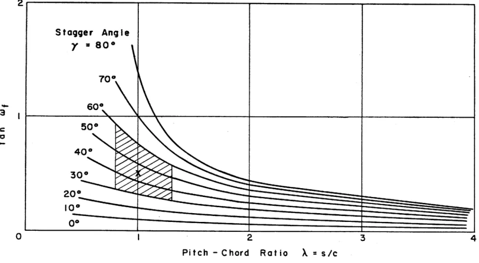
t~2oK~vl

Fig. I shows the result of a numerical calculation of the above equation, which gives the correction Values for the circulation due to the change of

axial velocity as a function of pitch-chord ratio )\ and stagger angle . Now, from the following figure, a concrete method can be suggested:

for correcting the velocity tri-angles in the case of accelerated or decelerated axial velocity to that of constant axial velocity. The practical drawing method is as seen at the left. Suppose the prescribed velocity triangle

_____ is as shown by arrows (solid lines)

of the Figure. First, we draw the mean axial velocity line m - m.

Second, from the tops of both arrows, draw two parallel straight lines L - L and L' - L', which Are inclined to the axial direction by an angle .

(A~I

has the following physical meaning.

The values of

Wf

can easily be found in Fig. 1, if the values of pitch-chord ratio

?\

and stagger angle i are known. Then, the two points of in-tersection of the lines m - m and L - L, m - m and L' - L' correspond re-spectively to the velocity vectors at the inlet and exit of the cascade with a constant axial velocity. In Fig. 1, the most useful domain for

practical purposes is shown by the shaded area. In this domain, tan

Wf

seems to vary from 0.3 to 0.9, and for the most practical purposes it will

be enough to put tan

Wf

= 0.5 for the usual xial flow compressor design.

2 -

6.

Correction of the Turning Angle

In the procedures of the foregoing considerations, the mean of the inlet and exit velocity vectors is taken as the standard velocity, for the

to get is the turning angle through the cascade keeping the inlet velocity vector constant. Therefore, it would be necessary to refer to the method of turning angle correction in order to keep the inlet velocity vector

con-stant.

It has already been proven elsewhere

(8)

that the following general relationship holds for all kinds of cascades.

Where, Pl is the inlet velocity direction measured. from the axis, 32 is the saae one at exit, and

Q

,

(1

are the constants peculiar to the prescribed cascade profiles and their physical arrangements. Q0 and

17/ are expressed by the following eqUations, if the conformal mapping of their boundaries into the unit circle is possible (9).

Now, let the values of Pl', 2 which are obtained by the drawing procedure and shown in the foregoing paragraph to be 10 and

P20

respectively, and expand both sides of Eq. (24) in a Taylor Series, that is;

approximating relation

Putting,

we obtain this relation:

,)

C'

(2-6)

The above equation is valid for all kinds of profiles, and in the case of a flat plate cascade, we can deduce Eq. (26) from Eq. (1) and (8). Using the above result, we can obtain the correction values d 12 of the exit angle 32, which correspond to the required change d 1 of the inlet angle 3. Fig. 2 shows the values of e for flat plate cascades as a function of pitch-chord ratio X and stagger angle 1 . It can be seen from this figure, that in the vicinity of a pitcU- chord ratio .

= 1, all of the

values of

TJ

are very near 0.05. This means, for normal values of turn-ing angle, the correction value O 2 of the exit angle is nearly 0.10 per

2

degree of inlet angle adjustment. Therefore, in most cases, it does not seem necessary to correct the exit angle. However, in the case of pitch-chord ratio larger than 1.2 and large stagger angle such as = 60*, the values of exit angle correction might exceed 0.5* or more per degree of inlet angle adjustment. In such cases, correction of exit angle should

A\h

A

/

the first approximation as sufficiant

To approach the more practical

solution, let's consider the flow

through cascades composed of ar-bitrarily shaped blades. There are several methods to solve such a problem involving a small per-turbation based on the solution of flat plate cascades. In this paper, one of the simplest

approxi-mation theories similar to the

Hudimoto method (6) shall be a-dopted. Since we requipe very

small quantities in the final

result, we shall consider only for our purposes.

3 - 1. General Equations

Consider a cascade composed of an arbitrary blade shape such as the figure above. The whole blade shape is supposed to be prescribed by the following equation

Now let's consider the source distribution corresponding to the axial

velocity change from v to v . Restricting our problem to the case of

uniformly distributed sources, the strength of source per unit area

9

one passage between two adjacent blades is,

6z=

C

S(

c

s

T",O-

A)

and this must coincide with the change of axial velocity before and after

the cascade, therefore,

O/'- 2 -

'1/3a I S -= 1( S C cis -Ir

-

A)

hence, ('- /)

(

c

s COVs

-

A

Finally, using Eq. (4), the apparent change of axial velocity is given by the following equation.

-

-

(29)

where

c s

cs

-e

B is the "blocking ratio" of the passage by the blade, and in the usual

case of the axial flow compressor cascade, it has always small value

around 0.1.

Then, the local apparent axial velocity change A&6 at any point P on the blade surface, brings a normal velocity component

4V9I

to the blade surface at this point.

The relation between

A'4,

and jML is as follows,

All? e Sl (6+'

lop

Ai

----

(3 0)

where,

_d

_i

and

5'

is given numerically, since the blade shape is prescribed by Eq. (27). Assuming &(<I , so that X

O 4 , V becomes

as follows.

In the above equation, the second term on the right hand side is the same as Eq. (5). Therefore, all we have to do, is to solve for the first term

only, and superimpose it onto the solution of a flat plate cascade. Now,

considering the first term only, the radial velocity distribution around the unit circle becomes,

de dy

-d(+)

d &

CI-0

_

CP

On the other hand, let's consider the flow which cancels the normal ve-locity around the unit circle. First, to satisfy the boundary condition, a quantity of fluid

J,

must be sucked into the unit circle. Further-more, considering that the quantity of fluidq-A must be sucked into

the blade from an infinite distance in both directions perpendicular to

the cascade axis, the following complex velocity potential function is given.

where I

' -7

Using Eq. (28) the above equation can be rewritten in the following form.

Chere-

AB

__

4rI-a

Is K

From the above equation, the radial velocity v and the tangential velocity

r

V0 Onl the unit circle become:

_

c

VCI

AB

I-8

n -

,-8

-vi

K C2M

S

2-C(WIM

_c

n

_{( E, Cos n}

_0,

_F.S#,n"6'9)

_-

_--

_{- (34-IA)}

4o (

'V =-C

'S

Z n

E

n

3M6

Therefore, setting Eq. _{(32) and Eq. (34-A) equal, we can determine the} values of the Fourier Series

Ers

and

d

9rgOt

Fr

as follows.

.

e

C, s

AS

-A

-

-1-8

132-r

K

C4

2

G

Now, we can calculate the tangential velocity on the unit circle using

Eq. (34-B) and the determined values of

En

and F,,

At the trailing edge,

00

C

M

-

)

ne-

-

(36)

However, the tangential velocity at the trailing edge, due to the

com-plex velocity potential given by Eq.

(36) and

(37),

'p

-41r

27r

K

can be determined as follows.

Zlr

('~$~L-

'v~,)

S

K

~i

(3~&)

(13)

is;

From Eqs.

?rO Cos

n

')- - - -(34-

8)

(I

W

o

0=

0

VzO S

Now we can calculate the value of the circulation, which corresponds to the first term of Eq. (3l). Therefore, superimposing this onto the solu-tion of the flat plate cascade, we can calculate the correcsolu-tion value for the circulation in the case of an-arbitrarily prescribed blade profile.

3 - 2. Calculation for NACA 65 - Series Compressor Cascades

Since the calculation for each case is a rather laborious one, for

convenience it is preferable to make some numerical graphs for certain blade profile series. In this paper, numerical graphs for the rapid characteristic estimation of NACA 65 - Series Compressor Cascades were prepared. NACA

65

- Series blade profiles consist of a camber line and

thickness distribution, and both values change proportionally to some

"designation" with the distribution remaining constant. The designation

for camber line is CCO , which expresses the lift coefficient in

the case of an isolated wing. The designation for thickness is the "value

of the maximum thickness", and in this paper, let us designate it 4empo-rarily t.

Now, as it can be seen from the above description, taking the chord line as the abscissa x, the ordinate y on the blade surface can be ex-pressed by the following equation:

V h !/C

where, j1 represents the ordinate of the camber line,

9t

represents

the ordinate of thickness only, the + sign is taken for the upper surface

and the - sign for the lower surface. Furthermore, we can write:

Hence,

d

= CI X

(

, -)

dX

_{dZ C',= .~ D}

d-yt

----

(39)

where B0 is a blocking ratio corresponding to to and to is some standard thickness ratio.

Substituting Eq.

_{(39) into}

Eq.

c(

n

Pi+

Fsttn )

(35)

we can write,

d(

-C)

C0

)CW

k

SB

1-13

f

.

d(1)4

,

8.

do

C

27r

27r ,

Then, we divide the above equation into two parts as follows:

n~'

Pi

Z.(@ _E'

Vo.

-a

B

I-.,

Finally, putting

t~in

OL

7

_T

A

K

he ol

We get the following conclusi-ve equation

7'VC,,

to

)

4

t-'i A,

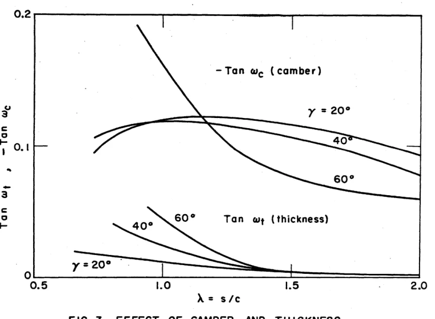
In Fig.

3,

tan

(&A

and tan 4* are shown for the case of

Cco

=

/-0

,

t = 0, and C10 = 0, t = 0.1 respectively. It can be seen from the previous

description that the solutions for all other combinations of C10 and t can be easily found from this numerical graph.

'I:.

to'st

Ich

C

is.

dip

Col

z

elms~

d~fe4*

4'#*

C )

9

Fn

4. CORRECTION FOR SECONDARY FLOW

As was briefly mentioned in the introduction, secondary flow occuring in the passages of a cascade due to boundary layer causes the deviation of turning angle. _{Usually, this factor can be considered almost independent} of the phenomena considered in previous sections.

Therefore, to reach a more accurate solution, we must add the cor-rection value for secondary flow to our calculation. For the corcor-rection

of secondary flow, it is considered appropriate to use the Otsuka's method (10). Otsuka developed the secondary flow theories built by Squire-Winter (11), Preston (12), and Smith (13), and devised a convenient formula to estimate the deviation of turning angle due to the secondary flow in the passages of cascades.

According to his theory, deviation of the turning angle

S

owing to the secondary flow can bp calculated by the next equation.

* |d4 CoSI~(s vT

Where, _{INrIM is the magnitude of average inlet velocity along the span,} hbt/ _{is the locally accelerated inlet velocity caused by the existence} of a boundary layer on the inelt side wall.

Using Eq. (40) and the experimental value of A , we can estimate the value of , _{which must be superimposed into our}

cal-cUations. Fig. 4 shows the values of S U for various inlet angles and exit angles j3

5.

NUMERICAL EXAMPLES

To confirm the validity of the theory, comparisons were made with

several sets of experimental data. All of the experimental data here

used (14),

(4),

(15) were collected from the publications on hand. All

of the data were for NAQA

_{65 Series Compressor Cascades}

_{using low speed}

wind tunnels.

In them, turning angles are plotted against

_{attack angles}

for the cases of both solid wall and porous wall. In the latter case,

two-dimensional flow is supposed to be maintained at the middle of the

span.

_{For both cases, all data gave the rate of axial velocity chazige}

'1 / , before and after the cascades. Now starting with the

value fdr solid wall, what we want to do is to correct the effect of

sec-ondary flow and the effect of axial velocity change on them, and to

com-pare the final curve to that of the porous wall.

In the first group of data (14) (from Fig. 5 to

Fig. 10), the value

of

W

was estimated to be 0.03, according to the velocity

distribution shown in the report.

In all figures, thin solid lines express

the value for the porous wall, thin dotted lines show the value for the

solid wall, while thick solid lines show the results of calculations

started from solid wall data.

Since the NASA porous wall data (4) (Fig. 11) uses a somewhat

dif-ferent value compared with the other report (15), in this paper the value

of the latter was adopted as the value of the porous wall experiment. The

last data (Fig.

12) came from M.I.T. (16) and in this

cast, as the data

of a decelerated case was also presented, it was used in comparison, and

the result is given by the dbt-dash line in the figures. In the

deceler-ated case, since the secondary flow theory no longer has its meaning, the

correction for the secondary flow was omitted. In both the NASA and MIT data, because of the lack of _{description of inlet velocity distribution,} it was assumed that = 0.1 temporary.

6. CONCLUSIONS

In this paper, a general method was developed for the evaluation of cascade performance with accelerated or decelerated axial velocity. For the series of NASA 65 Series Compressor Cascades especially, numerical graphs for practical use were presented. From the comparison of the theory with- the datafrom several experiments, we see that good

agree-ment exists between them. However, there still remains some descrepincy. On the one hand, it seems to depend upon the accuracy of the cascade test-ing technique itself: on the other hand, the more complicated factors

such as the effect of viscosity might affect the performance, which is beyond the scope of the present treatment. Restricting the discussion to the procedure treated here, the accuracy of the calculation would be

doubtful in the more highly cambered blade or in a narrower spacing than the present example, because of the invalidity of the simple conformal transformation function used. Fortunately, such a difficult case would not appear frequently in the practical design of axial flow compressors.

BIBLIOGRAPHY

1. Scholz, N. "Two Dimensional Correction of the Outlet Angle in Cas-cades Flow', Journal of Aero. Sciences, Vol. 20, 1953.

2. Katzoff, S., Bogdonoff, E. H., Boyet, H., "Comparison of Theoretical and Experimental Lift and Pressure Distribution on Airfoils in

Cas-cades", NACA TN 1388, 1947.

3. Hawthorne, W. R., "Induced Deflection Angle in Cascades", Reader's Forum, Journal of Aero. Sciences, Vol. 16, No. 4, 1949.

4. Erwin, J. R., Emery, J. C., "Effect of Tunnel Configuration and Test-ing Technique on Cascade Performance", NACA TR 1016, 1951.

5. Kawasaki, T., "Some Tests on Cascades of a Compressor Blade", Journal of the Japan Society of Mechanical Engineers, Vol. 22, No'. 113, 1956. 6. Hudimoto, B., Kamimoto, G., Hirose, K., "Theory of Wing Lattice",

Tech-nical Reports of the Engineering Research Institute, Kyoto University, 1952.

7.

Hirose, K., Hudimoto, B., Trans. pf the Japan Soc. of Mech. Engineers, Vol. 4, No. 27.

8. Traupel, W., "On the Potential Tapory of Blade Cascades", Sulzer

Re--view, 194.t

9. Kubota, S., "Aerodynamic Researches on Turbine Cascades", Technical Report, Kawasaki Dockyard Co., 1958.

10. Otsuka, S., "A Theory about the Secondary Flow in Cascades", Proceed-ings of the 6th Japan National Congress for Applied Mechanics, 1956. 11. Squire, H. B., Winter, K. G., "The Secondary Flow in a Cascade of

Air-foils in a Non-uniform Stream", Journal of Aero. Sciences, Vol. 18, 1951. 12. Preston, J. H., "A Simple Approach to the Theory of Secondary Flows",

The Aero. Quarterly, 1954.

13. Smith, L. H., "Secondary Flow in Axial-Flow Turbomachinery", Trans. of ASME, 1955.

14. Takeya, K., "On the Wind Tunnel Tests of Compressor Cascades with Boundary Layer Suction", Presented at the Conference of Turbo Jet En-gines, Japan Society of Aero. Engineering, June 1956.

15. Herrig, L. J., Emery, J. C., Erwin, J. R., "Systematic Two-Dimensional Cascade Tests of NACA 65-Series Compressor Blade at Low Speeds", NACA

TN 3916, 1957.

16. Montgomery, S. R., "Three-Dimensional Flow in Compressor Cascades", MIT Gas Turbine Laboratory Report No. 48, 1958.

Stagger Angle

y

=

80*

N

700

600*\

500

40

300

x

200

100

00

K

2

Pitch - Chord

Ratio

X

= s/c

FIG. I CORRECTION OF CIRCULATION AROUND BLADES

FOR AXIAL VELOCITY CHANGE

1*.

3

C 0 I,-.

0

I I

3

4

I

I

70*

700

500

_______________________ .1 I

2

Pitch

-

Chord Ratio

X

=

s/c

FIG. 2

CORRECTION

OF TURNING

ANGLE

a0,

0.5

0

3

4

-

-

--

-IS I I I I I I I I I I I I I I I

-Z

OO

-90

I

-Tan

Cc

(camber)

3

y

=20*

0.1

600

3

4*

600

Tan wt (thickness)

020*

0.5

1.0

1.5

2.0

x=

s/c

400

200

1i=00

_500*#

600*

.0,5

E

1.0

700

-1.5

_{-- 1}

100

200

300

400

FIG.4

CORRECTION OF TURNING ANGLE FOR

65(216)-410,

y

=30*

-

s/c =1.25

C

-Solid Wall

Porous

Wall

/

Theory

0

₂₀

₈₀

a

120

0 N 0

1.2

65(216) -410,

y

= 50*

s/c =

1.25

7-1

711

1.0

-10

0 N

60

20

O0

160

Solid Wall

'

Theory

Porous Wal

I

I

I

I

I

20

8

0 0

a

120

FIG. 5 CORRECTION

BY THEORY.

OF TURNING

EXAMPLE

ANGLE

I

FIG. 6 CORRECTION OF TURNING

BY THEORY.

EXAMPLE

I.

21

0 N 0

1.01

149

10

0

04

20

0

160

ANGLE

2

I

-

-65 (216) -(12)10

y

= 30*

s/c

=

1.00

Solid Wall-*/,,

PouT

hesory-Porous Wall

80

120

a

160

0u Np

1.2

I

I

I

I

I

I

I

/

00 (2-10 ) -t( 1 I)V

y=

4 0

*

s/c = 1.00

171"

-

-\.0L

26

0

r-220

Nm

18*1

140

10*

200

-7

Solid Wall

-/

Theory

Porous Wall

F-

/

40

80

120

a

160

FIG.

7 CORRECTION

OF TURNING

BY THEORY.

EXAMPLE

3

ANGLE

FIG.8 CORRECTION OF TURNING

ANGLE

BY THEORY.

I

.2_-0 N N a

1.0

2

8*

2401

Ny

200

I80

120

40

200

I

EXAMPLE 4

7.01

65(216)

-(12) 10

y =

50*

s/c = 1.00

Solid Wall

/ Theory

Porous Wall

-

I

80

120

ax

160

1.4

a -N 0"

1.2

65 (216) -(20)10

y

=

30*

s/c = 1.00

32*

Nm

28

0

240

200

200

10

a

140

/

/

7

Solid Wal

A-Theory

Porous Wall

-

I

-I

180

a

220

FIG.9 CORRECTION OF TURNING ANGLE

BY THEORY

EXAMPLE 5

FIG. 10 CORRECTION

BY THEORY.

OF TURNING ANGLE

EXAMPLE

6

-0 >N

1.2

l.Ot

25*r-210

AN

70

90

4*

I

260

I

13*0

|

-

---NACA 65-12- 10,

A

=600

s/c = 1.0

Solid Wal l

z-

_Theory

Porous Wall

I

I

I

I

I

I

I

100

FIG.

II

CORRECTION

BY THEORY.

140

a

180

OF TURNING

EXAMPLE

a N a

1.2

F-1.0

1

8

0

r-Acc

e

l.

.- -Decel.

NACA 65 -4-10,

y

=450

s/c =

1.0

_{Solid Wall}

/

14*0

N

CQ

20

240

ANGLE

7

10.

/

Theory (Accel.)

X

-

T

heor

y

(Dece 1.)

Solid Wall (Decel.)

Porous Wall (Accel.)

-50

90

130*

1.0

0.8

170

a

FIG. 12 CORRECTION OF TURNING ANGLE

BY THEORY.

EXAMPLE 8

_m >p

1.2

l.0

240

N c

200

I 601

I 2

0

F-60

---10*0