UNIVERSITÉ DE MONTRÉAL
EFFECT OF LOAD ON MACHINE GEOMETRY WITH RESPECT TO THE
WEIGHT AND TORQUE
BEHKAM ASADISHAD
DÉPARTEMENT DE GÉNIE MÉCANIQUE ÉCOLE POLYTECHNIQUE DE MONTRÉAL
MÉMOIRE PRÉSENTÉ EN VUE DE L‟OBTENTION DU DIPLÔME DE MAÎTRISE ÈS SCIENCES APPLIQUÉES
(GÉNIE MÉCANIQUE) JUIN 2014
ÉCOLE POLYTECHNIQUE DE MONTRÉAL
Ce mémoire intitulé:
EFFECT OF LOAD ON MACHINE GEOMETRY WITH RESPECT TO THE WEIGHT AND TORQUE
présenté par : ASADISHAD Behkam
en vue de l‟obtention du diplôme de : Maîtrise ès sciences appliquées a été dûment accepté par le jury d‟examen constitué de :
M. BALAZINSKI Marek, Docteur ès sciences, président M. MAYER René, Ph.D., membre et directeur de recherche M. GOSSELIN Frédérick, Doct., membre
DEDICATION
I would like to dedicate this thesis to my family. I am very thankful for all of your support and encouragement during my studies.
AKNOWLEDGEMENT
I would like to acknowledge my advisor, René Mayer, for his invaluable guidance, supports, and encouragement. It has been an honor to work with him. I thank Mechanical Engineering faculty and technicians in Manufacturing Laboratory, Guy Gironne and Vincent Mayer for their companionship. I also thank my family, for without their support this degree would never have been possible.
I would also like to acknowledge the funding research association, Recherche et Innovation Synergétiques en Aérospatiale (CRIAQ), for supporting my research.
RÉSUMÉ
Dans cette étude, une méthode est développée pour estimer et prédire les coefficients d'erreur de la déformation d‟une machine CNC à cinq axes sous différentes conditions de chargement. Pour étudier l'effet de différents poids et les couples sur les erreurs de la machine, les blocs lourds identiques (10 kg chacun) ainsi que des entretoises lumière ont été conçus et fabriqués. Aprés installer les bocs et les boules sur la palette, la machine sonde les boules pour différents angles indexés par rapport à ses deux axes de rotation (B et C axes)en utilisant les codes G générés par programme RUMBA (the 3D reconfigurable uncalibrated master balls artifact). Au total, il y a 26 types d'erreurs et chaque erreur a maximum de cinq coefficients qui sont appelés coefficients d'erreur estimés. Les données obtenues à partir de la machine sont traitées afin d'estimer les valeurs des coefficients d'erreur pour chaque erreur. Ces derniers permettent d‟obtenir les graphiques polynômes de chaque erreur en utilisant leurs coefficients d'erreur. En outre, la matrice de corrélation de Pearson est obtenue pour tous les coefficients d'erreur et des poids et des couples. Les éléments de la matrice de corrélation (entre -1 et 1) indiquent le degré de dépendance de chaque coefficient d'erreur pour les autres coefficients, ainsi que le poids et le couple. Enfin, le procédé d'ajustement de la courbe est utilisé pour modéliser chaque coefficient d'erreur en fonction du poids et du couple. Ceci permet de prédire la valeur du coefficient d'erreur pour toutes les valeurs de poids et de couple supprimant la nécessité l‟essai expérimental. L'analyse résiduelle (la différence entre les valeurs expérimentales et les valeurs prédites) est ensuite utilisée pour vérifier l'exactitude du modèle. Les résultats de cette étude montrent que cette méthode est suffisamment précise pour estimer les erreurs de la machines qui est testés (HU40T machine CNC à cinq axes). Le modèle nous permet d'estimer les valeurs des coefficients d'erreur en fonction du poids uniquement, en fonction du couple uniquement et en fonction du poids et du couple simultanément. Cette connaissance est importante pour la compensation d'erreur ou la suppression d'erreur dans la machine pour augmenter la précision de la fabrication.
ABSTRACT
In this study, a method is developed to estimate and predict the error coefficients of a five-axis CNC machine tool deformation under different loading conditions. To study the effect of different weights and torques on the machine errors, identical heavy blocks (10 Kilograms each) as well as light spacers (less than 1 Kilogram) are designed and fabricated. After assembling the blocks and master balls on the pallet, the machine probes the balls for different indexations from the rotary axes (B and C axes) of the machine using G-codes generated from the 3D reconfigurable uncalibrated master balls artefact (RUMBA) program. In total, there are 26 types of errors and each error has maximum five coefficients which are called estimated error coefficients. The raw data obtained from machine is processed to estimate the values of the error coefficients for each error. Then, the polynomial function of each error can be achieved by using their error coefficients. Furthermore, Pearson‟s correlation matrix is obtained for all error coefficients and weights and torques. The elements of the correlation matrix (between -1 and 1) show the extent of dependency of each error coefficient to other coefficients as well as to the weight and torque. Finally, the curve fitting method is used to model each error coefficient as a function of weight and torque. The modeling allows predicting the value of the error coefficient for any weights and torques without doing an experimental test. Residual analysis (difference between the experimental and the predicted values) is then used to verify the accuracy of the modeling. The results of this study show that this method is accurate enough to estimate the errors of the tested machine tool (HU40T 5-axis CNC machine tools). The model enables us to estimate the error coefficient values as a function of weight independently, torque independently and weight and torque simultaneously. This knowledge is important for error compensation or even error removal in machine to increase the precision of the manufacturing.
TABLE OF CONTENTS DEDICATION………...iii AKNOWLEDGEMENT...iv RÉSUMÉ...v ABSTRACT...vi TABLE OF CONTENTS...vii LIST OF TABLES...x LIST OF FIGURES...xi LIST OF APPENDICES...xv CHAPTER 1. INTRODUCTION...1
1.1 Design and build means to apply controlled loading conditions...3
1.2 Determine the ball location for the RUMBA method and write appropriate G-code...4
1.3 Conduct the test...4
1.4 Analyze the error to identify possible patterns...5
1.5 Represent each error as a function of loading...5
CHAPTER 2. LOADING FIXTURES...6
2.1 Design stack...6
2.2 Assemble the blocks...8
2.3 Stack deflection...11
CHAPTER 3. RUMBA BALL LOCATION AND G-CODE...13
3.1 The mathematical model...14
3.1.1 Mathematical modeling of a joint motion...15
3.1.2 Mathematical modeling of a link...17
3.1.3 Nominal modeling...19
3.2 Generating G-code...23
CHAPTER 4. CONDUCT THE TEST...26
4.1 Machine tool...26
4.2 Master ball...28
4.3 Probe...29
4.4 Block...31
4.5 Spacer...31
4.6 Set of axes indexations...32
4.7 Validation test...36
CHAPTER 5. ANALYZE THE ERROR DATA...39
5.1 Polynomial graphs...39
5.2 Discrepancy of the errors...68
5.3 Volumetric Errors...74
CHAPTER 6. ERROR MODELING...76
6.1 Correlation...77
6.1.1 Correlation between the error coefficients...79
6.1.2 Correlation between the error coefficients and weight and torque...80
6.2 Curve fitting...81
6.2.1 Model the error coefficients as only a function of weight only...82
6.2.2 Model the error coefficients as only a function of torque only...84
6.2.3 Model the error coefficients as a function of weight and torque...86
6.3 Goodness-of-Fit Statistics (residual analysis)...88
CONCLUSION...94
Polynomial graphs...94
Correlation...95
Curve fitting...95
REFERENCES...98 APPENDICES...101
LIST OF TABLES
Table 2-1: The tests specifications...10
Table 2-2: The values of maximum deflection and the angle of the deflection for all tests...11
Table 4-1: Standard Features of the machine tool...26
Table 4-2: The probe components...29
Table 4-3: The nominal master ball coordinates for different tests...34
Table 6-1: All the possible error coefficients...76
Table 6-2: The 83 estimated error coefficients...77
Table 6-3: Correlation matrix for weight and torque...80
Table B-1: The estimated value of the error coefficients...122
Table D-1: The elements of the Jacobian matrix...132
Table E-1: Correlation matrix...134
Table F-1_a: The elements of the matrix PA from EXX2 to ECZ1...152
Table F-1_b: The elements of the matrix PA from ECZ2 to ECC4...153
Table F-2_a: The elements of the matrix PB from EXX2 to ECZ1...154
Table F-2_b: The elements of the matrix PB from ECZ2 to ECC4...155
Table F-3_a: The elements of the matrix PB from EXX2 to EAB1...156
LIST OF FIGURES
Figure 2-1: Block...6
Figure 2-2: Spacer...6
Figure 2-3: The fully dimensioned block...7
Figure 2-4: The fully dimensioned spacer...7
Figure 2-5: Different assembly of tests...8
Figure 2-6: The maximum deflection of the blocks for each test...12
Figure 2-7: The angle of the deflection for each test...12
Figure 3-1: Master ball artefac...13
Figure 3-2: Probe...14
Figure 3-3: Mathematical modeling of a joint motion...16
Figure 3-4_a: Modeling of the link and its parameters...17
Figure 3-4_b: Modeling of the link and its axis location errors...18
Figure 3-5: The nominal kinematic chain of the 5-axis CNC machine tool...20
Figure 3-6: The exact kinematic chain of the 5-axis CNC machine tool...21
Figure3-7: Machine pallet position in B=0°,C=0°...24
Figure3-8: Machine pallet position in B=-90°,C=0°...24
Figure 3-9: The flowchart for generating G-code in RUMBA...25
Figure4-1: MITSUI SEIKI 5-Axis High Production Machining Center Model HU40T...28
Figure 4-2: The artefact master ball...28
Figure 4-4: Gildemeister-devlieg system-werkzeuge gmbh microset...30
Figure 4-5: The fabricated block...31
Figure 4-6: The fabricated spacer...31
Figure 4-7: The position of B and C rotary axes of the machine pallet ...32
Figure 4-8: 15 0f 19 axes indexations...33
Figure 4-9_a: Diagonal pattern of ball locations...34
Figure 4-9_b: 4 corners pattern of ball location...34
Figure 4-10: The validation test set up with only blocks...36
Figure 4-11: The validation test set up with blocks and spacers...37
Figure 4-12: The length variation of the magnetic ball bar Renishaw...37
Figure 4-13: The 2D schematic of the validation test...38
Figure 5-1: Different polynomial graphs...39
Figure 5-2: The rainbow colors of the polynomial graphs...41
Figure 5-3: The polynomial graphs of the error EXX...42
Figure 5-4: The polynomial graphs of the error EYX...43
Figure 5-5: The polynomial graphs of the error EZX...44
Figure 5-6: the polynomial graphs of the error EAX...45
Figure 5-7: The polynomial graphs of the error EBX...46
Figure 5-8: The polynomial graphs of the error ECX...47
Figure 5-9: The polynomial graphs of the error EXY...48
Figure 5-11: the polynomial graphs of the error EZY...50
Figure 5-12: The polynomial graphs of the error EXZ...51
Figure 5-13: The polynomial graphs of the error EYZ...52
Figure 5-14: The polynomial graphs of the error EZZ...53
Figure 5-15: The polynomial graphs of the error EAZ...54
Figure 5-16: The polynomial graphs of the error ECZ...55
Figure 5-17: The polynomial graphs of the error EXB...56
Figure 5-18: The polynomial graphs of the error EYB...57
Figure 5-19: The polynomial graphs of the error EZB...58
Figure 5-20: The polynomial graphs of the error EAB...59
Figure 5-21: The polynomial graphs of the error EBB...60
Figure 5-22: The polynomial graphs of the error ECB...61
Figure 5-23: The polynomial graphs of the error EXC...62
Figure 5-24: The polynomial graphs of the error EYC...63
Figure 5-25: The polynomial graphs of the error EZC...64
Figure 5-26: The polynomial graphs of the error EAC...65
Figure 5-27: The polynomial graphs of the error EBC...66
Figure 5-28: The polynomial graphs of the error ECC...67
Figure 5-29: Discrepancy of the errors in different tests...69
Figure 5-30: The maximum volumetric error...75
Figure 6-1: The error coefficients modeling as a function of weight...82
Figure 6-2: The error coefficients modeling as a function of torque...84
Figure 6-3: The error coefficients modeling as a function of weight and torque...87
Figure 6-4: The data fit and the residual graph for Fit 1...88
Figure 6-5: The data fit and the residual graph for Fit 2...89
Figure 6-6: The data fit and the residual graph for Fit 3...90
Figure 6-7-a: The residual analysis for error EYX2...92
Figure 6-7-b: The residual analysis for error EXB1...92
Figure 6-7-c: The residual analysis for error ECC3...93
LIST OF APPENDICES
Appendix І: Matlab programs………...……….101
Appendix ІІ: The estimated value of the error coefficients...121
Appendix ІІІ: The equations of nominal modeling, exact modeling and volumetric errors...123
Appendix ІѴ: The elements of the Jacobian matrix...131
Appendix Ѵ: Correlation matrix...133
Appendix ѴІ: The coefficients of the fitted curves...151
Chapter 1 Introduction
Five axes CNC machining is very popular in industry for fabricating complex parts in aerospace and other precision fields. In these machine tools, there are three linear axes (X, Y and Z axis) and two angular axes (the rotation of the pallet and the rotation of the cutting tool). The finished parts which have been machined by five-axis CNC machine tools, have smooth surface with high quality and high accuracy [1,2]. However, the presence of two rotary axes can increase the number of error parameters and decrease the machine calibration, especially when the direction of cutting tool is not parallel to the gravity. These kinds of machine tools are called Horizontal. Their cutting tool is horizontal and thus, the workpiece, the pallet, and the cutting tool are effected by their weights [3].
There are numerous studies regarding machine tools errors. In some studies, the circular test method has been used to measure the errors and diagnose the source of errors. For instance, Zargarbashi and Mayer assessed axis motion error using magnetic double ball bar[4]. In another study, Knapp used a new device called R-test to measure X-Y-Z deviations of circular and spherical movements to calibrate parameter errors such as backlash, positioning error, squareness and parallelism [5]. Hong et al presented a method to identify the motion error sources (non-directional error pattern and (non-directional error pattern) by using circular test [6]. Some other studies investigated the accuracy of the machine tools. For instance, Lei and Hsu presented an error model in the template of homogenous transformation matrix (HTM) and did accuracy tests on a 5-axes CNC machine tool with 3D probe-ball [7,8]. Lu et al presented a new two-dimensional method to investigate the existence of radial error motion in the spindle [9,10]. Iwai and Mitsui developed a method to determine 11 error parameters created by the link length and the inclination of the link axes using rotary encoders and link mechanisms [11]. Yang developed a multi-probe measurement system to investigate the motion accuracy of high –precision micro-coordinate measuring machine [12]. In some studies, the laser interferometer has been used for measuring the positiong errors in machine tools. Ziegert and Mize developed a method to map the volumetric positioning error by using the laser ball bar (LBB) consisting of a laser interferometer aligned with a telescoping ball bar [13]. Castro and Burdekin developed a method to evaluate the positioning accuracy of machine tools and CMM [14]. In recent studies, machine tools have been calibrated by probing the artefact master balls to measure the error parameters during machining.
Erkan and Mayer analyzed the volumetric errors of a five-axe CNC machine tool by probing an uncalibrated artefact [15,2]. Mayer and Erkan also calibrated the 5-axis machine tools by using reconfigurable uncalibrated master balls artifact (RUMBA) [1]. However, there are limited studies on the effect of loading on machine tool errors.
In this project, we aimed to investigate the effect of load on machine geometry with respect to different torques and weights by installing different workpieces on the machine. This allows us estimating the error parameters during machining to compensate them or at least reduce the error values and increase the precision of manufacturing. The compensation can be done by adding the offset manually (in the generated G-code) or automatically (define the offset in the post-processor of the machine tool), fixing the position of the machine axes (such as guideway), etc. Thus, we will be able to recognize the significant machine errors and compensate them before the machining. After compensating the errors, the cutting tool will approach to the exact point of the part which is defined in the G-code file.
To this end, identical heavy blocks (10 Kilograms each) as well as light spacers (less than 1 Kilogram) were designed and fabricated. After assembling the blocks and master balls on the pallet, the machine probed the balls for different indexations from the rotary axes (B and C axes) of the machine using G-codes generated from the RUMBA program. In total, there are 26 types of errors and each error has maximum five coefficients which are called estimated error coefficients. The raw data obtained from machine is then processed to estimate the values of the error coefficients.
There are numerous error sources during machining. Some are systematic and may be compensated. However, the exact number of error parameters is unknown. It is thought that load-induced errors are more significant under certain conditions. In this study, 83 error coefficients which combine axis component errors and axis location errors have been investigated. [16]
The project methodology follows five steps:
1. Design and build means to apply controlled loading conditions;
2. Determine the ball location for the RUMBA method and write appropriate G-code; 3. Conduct the test;
4. Analyze the error to identify possible patterns; 5. Represent each error as a function of loading
1.1 Design and build means to apply controlled loading conditions:
Loading is quantified as force (weight) and related torque. A judicious use of weight units and stacking arrangements allow a sufficient variety of loading conditions for the subsequent analysis. A design based on a “standard” loading unit, a block, was selected. Each block is a ten kilogram steel piece.
When stacking the blocks, it is essential to verify that the combined deflection and tilt of the stack does not create excessive deviations in the master ball positions relative to the machine table. Thus, we have to calculate the maximum deviation and the angle of deviation in the assembled blocks. The stack is modelled as an end-fixed beam and the weight force is a distributed force. The maximum deflection occurs at the end of the beam.
To achieve various loading conditions, some spacers are inserted between the blocks and the table. The spacer is an aluminum piece with a cubic shape. The spacer must be as light as possible to minimize the effect of its weight since the objective of the spacer is to increase torque not weight.
The blocks have been designed and fabricated. The main block is made of steel and is machined. There are four islands at the corners of a block to have a more definite contact with each other and avoid rocking. There are four holes for fixing the blocks together and installing the master balls on them. The spacers also have four holes but have smaller dimensions (due to material stock availability).
1.2 Determine the ball location for the RUMBA method and write appropriate G-code RUMBA method allows using different master balls in different location of the pallet (Appendix Ι) [2]. Thus, the number of master balls and their location are adjustable and giving us an opportunity to have more access to different spheres in different combinations. There are some ways for calibrating the artifact master ball:
1. The ball center coordinate is measured as a nominal value. The nominal coordinates for other measurement locations are calculated. The difference between the measured and the calculated coordinates identifies the volumetric errors [17].
2. The artefact is calibrated on a coordinate measuring machine (CMM) and then probe on the machine tools. The difference between these two data can generate the error vectors [18].
3. A 3D artefact is created by mounting a 2D ball plate in different locations. The relation between machine errors and the uncertainty is used to predict the volumetric errors [19],[20].
Having the coordinates of each ball, the G-codes are generated to define the probe trajectory throughout the test. For each test, to probe the balls in different positions, the pallet needs to be rotated in C-axis by 360 degrees and in B-axis by 180 degrees (The B axis will be moved over its range of -90 to +90).
1.3 Conduct the test
All the tests are performed on HU40T 5-axis CNC machine tools. The experimental test is based on the probing the spheres in different combinations (the pallet rotates around its B rotary axes). The probe approaches to the spheres according to the G-code which is generated by RUMBA using Matlab program. The following limitations should be considered:
1. The available blocks:
12 blocks and 4 spacers have been fabricated with respect to the range of Z axis in the HU40T five axis CNC machine tools.
2. The HU40T standard specification:
All twelve tests have been designed regarding to the machine tools limitation. The maximum possible weight that can be installed on the pallet is 100 kilograms. The maximum distances for Z axis and X axis are 300 mm and 600 mm respectively.
1.4 Analyze the error to identify possible patterns
After experimental tests, we are able to process the data and estimate the error parameters. With the processed data, it is possible to plot the polynomial graphs of each type of motion error for different loading conditions (different tests). In this section, the goal is to find a possible pattern between load and error values.
1.5 Represent each error as a function of loading
In this chapter, the objective is to find the correlation matrix to show the level of dependency between the error coefficients and weight and torque. The most correlated error coefficients are identified. Then, each error can be defined as a function of load, torque and both of them simultaneously. Thus, the value of each error coefficient can be estimated for any weight and torque. Finally, residual analysis is done to verify the accuracy of the modeling.
Chapter 2 Loading fixtures
To investigate the effect of load on the machine geometry, a loading system needs to be mounted on the pallet.
2.1 Design stack
The weight of different parts during machining creates a torque relative to the center of the pallet. The loading system consists of a set of standard blocks and standard spacers. This helps us to simultaneously monitor the trend of changes in machine errors with torque and weight by running the test with different weights and different torques. The block is a 10-kilogram steel piece. Figure 2-1 shows the designed block. The block has four holes for being fixed on the pallet or on the other blocks and 4 islands for fixing it on the other blocks and reduce rocking. Some of the blocks have extra hole at the center of the other holes that can be used for placing a master ball on the block.
For achieving more possible loading conditions, a spacer has been designed. The spacer is made of aluminum with four holes (for being fixed on the main blocks). The spacer has been hollowed out as much as possible to reduce the effect of the weight and creates maximum torque. Thus, we can do various tests with different weights and torques. Figure 2-2 shows the designed spacer. Figures 2-3 and 2-4 show the fully dimensioned block and spacer, respectively.
Figure 2-3: The fully dimensioned block
2.2 Assemble the blocks
The blocks have been assembled symmetrically to avoid creating torque around C-axis of the pallet. The possible patterns for assembling the main blocks and the spacers can be: Diagonal: The blocks are installed on a diagonal of the pallet.
Four corners: In this pattern the combination of blocks and spacers is placed at the corners of the pallet.
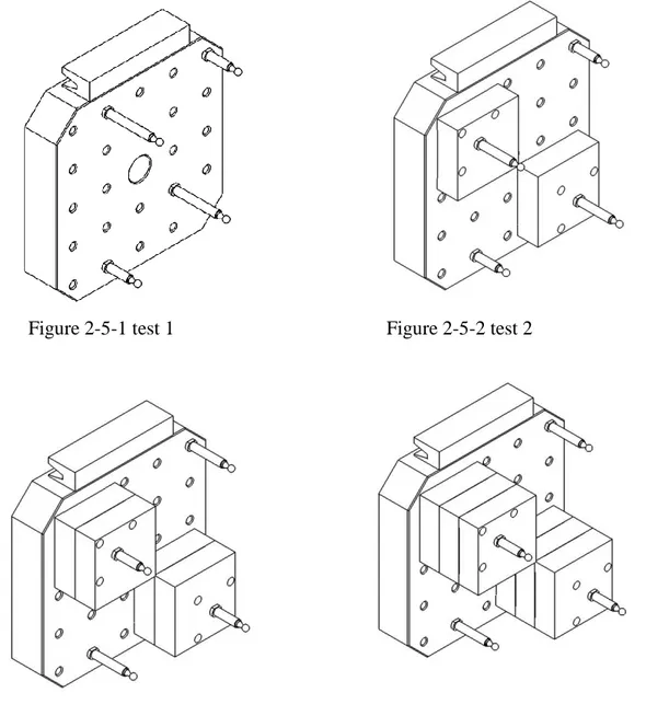
Figure 2-5 shows all the possible loading configurations with respect to the designed blocks and the limitations of the machine tools.
Figure 2-5-1 test 1 Figure 2-5-2 test 2
Figure 2-5-5 test 5 Figure 2-5-6 test 6
Figure 2-5-7 test 7 Figure 2-5-8 test 8
Figure 2-5-9 test 9 Figure 2-5-10 test 10
Figure 2-5-11 test 11 Figure 2-5-12 test 12 Figure 2-5: Different assembly of tests
Table 2-1 presents all the possible tests with the number of blocks and spacers and their patterns. The maximum weight that is permitted to be used on the HU40T CNC machine tools is 100 kilograms.
Table 2-1: The tests specifications
Tests Pattern Number
of blocks Weight(N) Torque(N.m) 1 No pattern 0 0 0 2 Diagonal 2 200 5 3 Diagonal 4 400 20 4 Diagonal 6 600 45 5 Diagonal 8 800 80 6 Diagonal 10 1000 125 7 4 corners 4 400 10 8 4 corners 8 800 40 9 4 corners 10 1000 75 10 Diagonal(with spacer) 2 200 20.1 11 Diagonal(with spacer) 6 600 90.3 12 Diagonal(with spacer) 2 200 35.2
2.3 Stack deflection
It is essential to verify that the maximum deflection of a stack of blocks and also the angle of their deflection do not create excessive deviations in the master ball positions, which are placed on the blocks, relative to the machine pallet. Equations 2-1 and 2-2 calculate the maximum deflection and angle of the deflection respectively:
y =
(2-1) , Θ =
(2-2)
y: maximum deflection (m) and Θ: angle of deflection (rad). Where w is weight force (N/m), L is
the total length of whole blocks (m), E is module of elasticity (= 200 GPa), and I is area moment
of inertia ( ).
With I =
=
=
95.415 = 3.97 ׄb‟ and „h‟ are the width and height of the blocks, respectively.
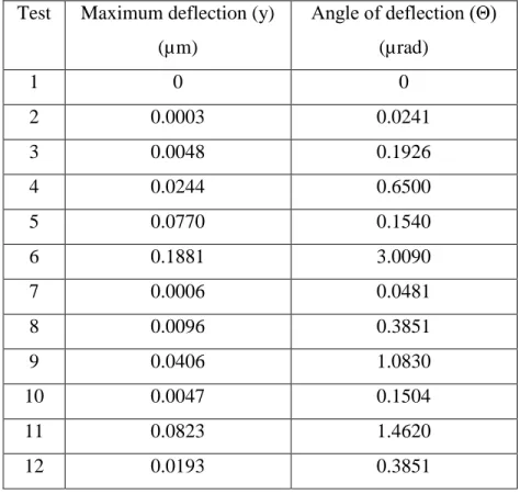
Table 2-2: The values of maximum deflection and the angle of the deflection for all tests
Test Maximum deflection (y) (µm) Angle of deflection (Θ) (µrad) 1 0 0 2 0.0003 0.0241 3 0.0048 0.1926 4 0.0244 0.6500 5 0.0770 0.1540 6 0.1881 3.0090 7 0.0006 0.0481 8 0.0096 0.3851 9 0.0406 1.0830 10 0.0047 0.1504 11 0.0823 1.4620 12 0.0193 0.3851
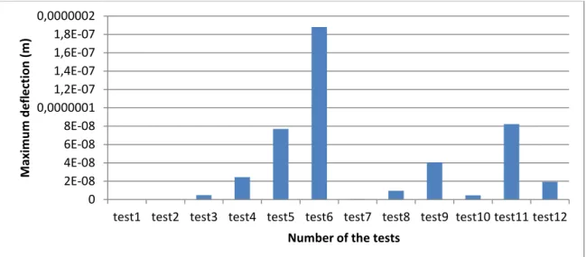
As shown in table 2-2, the maximum deflection was for tests with huge load and huge torque. However, the maximum values for the deflection and the angle of the deflection in theory are 0.1881 (μm) and 3.0090 (μrad), respectively. Thus, the tests did not create excessive deviations. With above values, it is possible to sketch the graph and show the trend of maximum deflection and the angle of deflection. Figure 2-6 and figure 2-7 are histograms of the linear and angular deflection.
Figure 2-6: The maximum deflection of the blocks for each test
Figure 2-7: The angle of the deflection for each test
0 2E-08 4E-08 6E-08 8E-08 0,0000001 1,2E-07 1,4E-07 1,6E-07 1,8E-07 0,0000002
test1 test2 test3 test4 test5 test6 test7 test8 test9 test10 test11 test12
M axi m u m d e fl e ction ( m )
Number of the tests
0 0,0000005 0,000001 0,0000015 0,000002 0,0000025 0,000003 0,0000035
test1 test2 test3 test4 test5 test6 test7 test8 test9 test10 test11 test12
A n ge l o f d e fl e ction ( rad )
Chapter 3 RUMBA ball location and G-code
RUMBA method uses a combination of master balls on the machine pallet to probe the data [2]. In this method, the number of master balls and their location on the pallet are adjustable. This flexibility helps to probe the master balls for different rotary axes indexations.
Four master balls are used in each test with the same location in X-Y plane to maximize consistency between the tests. We tried to keep the test conditions constant to achieve more accurate results. The length of each master ball can be changed in each test (to facilitate their access for probing). In some tests (with four corners pattern), it is necessary to slightly change the ball location.
The artefact combines sphere, ball plate and magnetic link. The artefacts have been calibrated by calibrating the ball plate and the magnetic ball link separately on CMM. Figure 3-1 shows an artefact.
Figure 3-1: Master ball artefact
In RUMBA method, the master balls do not need to be calibrated with the CMM. Thus, they were placed on the pallet without any calibration.
The probe was mounted in the tool holder (cutting tool) of the machine tool. Figure 3-2 shows the probe, made of MP 700 by Renishaw. The machine probed each ball to determine its exact coordinate from five touches, four at the equator and one at the pole. The points on the equator
were along 45° diameter. This increases the accessibility of touch points in a variety of artefact locations.
Figure 3-2: Probe
The measurements can vary in different runs and can be influenced by other factors such as thermal effect.
Repeatability: to verify the repeatability of machine tools, each test was done at least 3 times.
Thermal effect: The temperature of the machine tools may change during the test. This can affect the accuracy of the results. To minimize the thermal effect and to be consistent, all the tests which last two and half hours were done in the morning when machine was cold.
3.1 The mathematical model
The mathematical model has been designed for the HU40T five-axis CNC machine tools. This model represents the nominal modeling, exact modeling and the approximate modeling of the 5-axis CNC machine tools to estimate the values of the error parameters. Before presenting the model, the mathematical model of a joint motion and a link will be calculated.
There are a lot of error sources in machine tools such as geometric deviation, thermal effects, elastic deformation, dynamic effects, NC related errors [16]. The following list defines each type of error:
Geometric deviation exists in guideways, links and structural elements which can be compensated by physical modification of the machine tools.
Thermal effects which are caused by heat originating from machine motor, coolant system and the environment. Thermal errors can be classified as quasi-static errors which change slowly in time and are related to the machine structures [21]. This type of error can be reduced by using the machine in a known time and by the maintenance of the motor, guiding system and coolant system.
Elastic deformations in workpiece or even machine elements such as cutting tool, weight and guideway because of forces.
Dynamic effects because of inertial forces.
NC related errors can happen because of the machine tools internal interpolation. NC command is the main part of each machine tool where all the G-code programs are translated to the machine language there.
In this work, only the geometric deviations are considered: Mathematical modeling of a joint motion
Mathematical modeling of a link
3.1.1 Mathematical modeling of a joint motion
Figure 3-3 shows the nominal X axis (X) and its polynomial curve (actual trajectory ). In this figure, the linear error (black vector) is ( ⃗⃗⃗⃗ ) and the angular error (red vectors) is ( ⃗⃗⃗ ).
Figure 3-3: Mathematical modeling of a joint motion (black vector is the linear error ( ⃗⃗⃗⃗ ) and the red vector is the angular vector ( ⃗⃗⃗ ))
Equation 3-1 indicates the relation between the actual coordinate of and the nominal coordinate in machine frame and X frame respectively.
{ } = + (⃗⃗⃗⃗ +
́ { ́} ́ ) (3-1)
( ⃗⃗⃗⃗ ) is the linear error matrix and (R) is the mobile frame rotation. ( ) is the distance between the reference point (zero point) and the nominal joint. (R) in the above equation is equal to:
= I =[
] (3-2)
́ = rot(ECX, ̂)rot( ̂)rot( ̂) =rot (ɣ,z) rot (β,y) rot (α,x) (3-3) rot(ECX, ̂) = rot (ɣ,z) = [
];
rot( ̂) = rot (β,y) = [
];
𝛿𝑥 ⃗⃗⃗⃗
rot( ̂) = rot (α,x) = [
];
Equation 3-1 is a vector form of a joint motion modeling. The mathematical model of a joint motion can be also written in homogenous transformation matrix form (HTM). Equation 3-4 represents the HTM model of a joint motion.
[ { } { } { } ] = [ ] [ ̂ ̂ ̂ ] [ { ́} ́ { ́} ́ { ́} ́ ] (3-4)
3.1.2 Mathematical modeling of a link
Figure 3-4 shows the model of one link with respect to its nominal and actual position. In this figure, the blue vector ( ⃗⃗⃗⃗ ) is a link error and the black vectors ( ⃗⃗⃗ ) are the axis location errors.
Figure 3-4_b: Modeling of the link and its axis location errors The vector form of the link model is presented in equation 3-5:
{ } = + [ ] + ([ ] + ́ ( +{ ́} ́ )) (3-5)
Equation 3-5 can be rewritten as equation (3-6):
{ } = [ ] + [
] + (rot ( ̂ ) rot ( ̂ ) rot ( ̂ )) ( [ ] + rot( ̂ )rot ( ̂ ) rot ( ̂ ) ([ ] + [ { } { } { } ] )) (3-6)
Where { } is the numerical component of vector projected in frame {X0}. „ ‟, „ ‟, „ ‟ are X offset of X, Y offset of X, Z offset of X respectively. „ ‟, „ ‟, „ ‟
are axis location errors of the Y-axis around the z, y and x axis respectively. The HTM for this model can be presented in equation (3-7):
{ } =
which can be expanded by equation (3-8): [ { } { } { } ] = [ ] [ ̂ ̂ ̂ ] [ ̂ ̂ ̂ ] [ ] [ { } { } { } ] (3-8)
The whole 5-axis machine tool is modelled by successively combining the two cited models of the joint motion and the link of the machine. The model of the cutting tool (spindle) and the workpiece have to also be considered in the modeling.
3.1.3 Nominal modeling
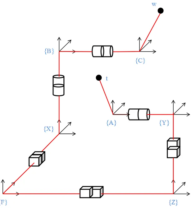
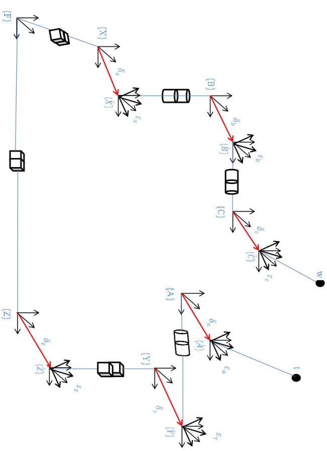
The HU40T five-axis CNC machine tool has a topology WCBXFZYST, where „W‟, „F‟, „S‟, and „T‟ are for workpiece, foundation, spindle and tool frame respectively. „C‟ and „B‟ represent the rotary axes of the machine; „X‟, „Y‟ and „Z‟ represent the prismatic axes of the machine. The nominal modeling of the machine presents the machine chain kinematic regardless to the errors of the machine. Thus, in the nominal machine, it is assumed that the machine works perfectly accurate. Figure 3-5 shows the nominal kinematic chain.
Figure 3-5: The nominal kinematic chain of the 5-axis CNC machine tool
3.1.4 Exact modelling
In the exact modelling, all the error parameters are considered. There are six errors (three linear and three angular) for each prismatic axes and there are also six errors (three radial motion, two tilt error motion and one indexation error angular) for each rotary axis of the machine tools. Figure 3-6 shows the kinematic chain of the exact modelling of the machine.
Below list presents all the motion errors from the exact modeling which can be occurred in the machine tools:
1. 'EXX' : Linear positioning error of X axis
2. 'EYX' : Straightness error of X axis in Y direction 3. 'EZX' : Straightness error of X axis in Z direction 4. 'EAX' : Angular error of X axis around X axis (roll) 5. 'EBX' : Angular error of X axis around Y axis (pitch) 6. 'ECX' : Angular error of X axis around Z axis (yaw) 7. 'EXY' : Straightness error of Y axis in X direction 8. 'EYY' : Linear positioning error of Y axis
9. 'EZY' : Straightness error of Y axis in Z direction 10. 'EAY' : Angular error of Y axis around X axis 11. 'EBY' : Angular error of Y axis around Y axis 12. 'ECY' : Angular error of Y axis around Z axis 13. 'EXZ' : Straightness error of Z axis in X direction 14. 'EYZ' : Straightness error of Z axis in Y direction 15. 'EZZ' : Linear positioning error of Z axis
16. 'EAZ' : Angular error of Z axis around X axis 17. 'EBZ' : Angular error of Z axis around Y axis 18. 'ECZ' : Angular error of Z axis around Z axis 19. 'EXA' : Axial error motion of A axis in X axis 20. 'EYA' : radial motion error of A axis in Y axis 21. 'EZA' : radial motion error of A axis in Z axis
22. 'EAA' : Angular positioning error motion of A axis around X axis 23. 'EBA' : Tilt error motion of A axis around Y axis
24. 'ECA' : Tilt error motion of A axis around Z axis 25. 'EXB' : radial motion error of B axis in X axis 26. 'EYB' : Axial error motion of B axis in Y axis 27. 'EZB' : radial motion error of B axis in Z axis 28. 'EAB' : Tilt error motion of B axis around X axis
30. 'ECB' : Tilt error motion of B axis around Z axis 31. 'EXC' : radial motion error of C axis in X axis 32. 'EYC' : radial motion error of C axis in Y axis 33. 'EZC' : Axial error motion of C axis in Z axis 34. 'EAC' : Tilt error motion of C axis around X axis 35. 'EBC' : Tilt error motion of C axis around Y axis
36. 'ECC' : Angular positioning error motion of C axis around Z axis
All the equations for nominal and exact modeling have been presented in appendix ΙΙΙ. 3.2 Generating G-code
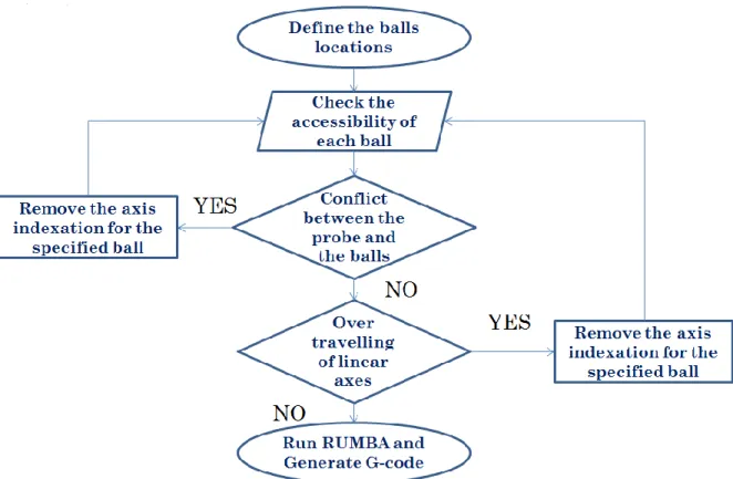
RUMBA method generates G-code after defining the balls locations and the accessible combinations (which ball can be probed and which cannot) [2]. The G-code is written according to the post-processor of the HU40T 5-axis CNC machine tool. In programming G-code, it is necessary to use right commands at the right place. Here, the commands are presented [23]:
N: The number of the blocks (N11 means the 11th block in G-code program) G: Functions related to the spindle motions.
1. G0: Rapid positioning 2. G01: Linear interpolation
3. G02, G03: Circular interpolation 4. G17, G18, G19: Plane selection 5. G90, G91: Position system
6. G20, G70, G21, G71: Length units (inch, mm) 7. G40, G41, G42: Tool Radius Compensation F: Feedrate function
M: Miscellaneous codes 1. M00: Program stop 2. M01: Optional stop 3. M30: Program end
4. M03: Spindle on and rotate clockwise
6. M05: Spindle off to stop
7. M19: Spindle off to stop at a certain angle S: Spindle speed function
T: Tool function
The RUMBA method uses the specific numbers to call the coordinates of each sphere in different rotary axes indexation. Here, a part of the G-code is shown:
#15=0.000000
#4=0.000000 The spindle (A-axis) rotation #9=1.000000 The number of the master ball #500=-90.000000 The B-axis rotation (°) #501=-180.0000 The C-axis rotation (°) #10=151.600000 The X location (mm) #11=120.000000 The Y location (mm) #12=120.000000 The Z location (mm) M19A#4 G0 B#500 C#501 G0 X#10 Y#11
We should take note that the coordinate frame changes in each rotary axes indexation which means that the axes have different directions during rotating the pallet. For instance, when the pallet is in B=0 and C=0, the linear axes are defined as shown in figure 3-7, but when the pallet moves to B= 90° , the axes will have a new direction same as in figure 3-8.
Figure 3-9 shows a flowchart for generating G-code in RUMBA. We should follow the flowchart to produce a right G-code.
Chapter 4 Conduct the test
4.1 Machine toolTests were conducted on a 5-axis machine tool in the laboratoire de recherche en fabrication virtuelle (LRFV) at École Polytechnique de Montréal. The machine is a MITSUI SEIKI 5-Axis High Production Machining Center Model HU40T. Table 4-1 presents the standard features of the cited machine.
Table4-1: Standard Features of the machine tool Working Capacity
Table longitudinal stroke (X axis) 610 mm (24.02") Spindle head vertical stroke (Y axis) 560 mm (22.05") Column travel stroke (Z axis) 560 mm (22.05") Interference of whole machine cover
with work piece on pallet
In machine 500 mm Ø (19.6" Ø)
In Optional APC 500 mm Ø (19.6" Ø)
Feed Rate
X, Y and Z axes 36,000 mm/min (1,417 IPM)
B axis 0.001°: 7,200°/min. (20 rpm)
C axis 0.001°: 7,200°/min. (20 rpm)
Cutting feed
X, Y and Z axes 0.1~20,000 mm/min. (0.004~787 IPM)
B axis 0.001°: 0.1~7,200°/min. C axis 0.001°: 0.1~7,200°/min. Minimum Resolution X, Y and Z axes 0.001 mm B & C axis 0.001° Power Required
Air required
Air Service Required 0.5 - 0.7 Mpa, 0.7 m3/min. (70 ~ 110 psi @ 25
cfm) (Dry and clean air) Air Service for 12,000 RPM Spindles and
Higher
0.5 - 0.7 Mpa, 1.0 m3/min. (70 ~ 110 psi @ 42 cfm) (Dry and clean air)
Machine Dimensions
Length 5,800 mm (229")
Width 3,930 mm (155")
Height 2,792 mm (110")
Machine Weight 13,500 kg. (29,700 lb.)
Numerical Control Equipment
CNC Control FANUC 30i MA
The experimental tests have been designed with respect to the machine‟s features. For instance, the maximum space for the blocks in Z-direction is 300 mm and each designed block has 50 mm height. Thus, it is impossible to put 7 blocks together on the pallet (the total height will be 350 mm). The other limitation is the maximum loads of 100 kilograms.
The G-code file is transferred to the NC of the machine. The NC reads the commands in the program and translates it to the machine language. Thus, the probe approaches to the exact position of the spheres. Figure 4-1 shows the HU40T 5-axis machine tool.
Figure4-1: MITSUI SEIKI 5-Axis High Production Machining Center Model HU40T 4.2 Master balls
Figure 4-2 shows one artefact master ball. These artefacts are used for probing. The artefact combines a sphere and a bar. At the base of the artefact, there is an adapter to screw it into the pallet holes. We can also install the master balls on the designed blocks with a thread changer. The material of the sphere is ceramic. The probe, which will be explained in the next section, touches the master ball five times to calculate the apparent position of the center of the ball. In this method, it is not necessary to calibrate the artefacts with CMM before probing. We only need to maintain the sphericity and the surface quality of the master balls [25].
4.3 Probe
The probe is a Renishaw MP700 with 360 degree transmission system. Spindle mounted optical transmission measurement probe is used for high accuracy component setting and inspection on medium to large machining centers. Table 4-2 gives the probe components.
Table 4-2: The probe components
MP700 probe 3D touch inspection probe
OMP optical module probe
OMM optical module machine
O-M-I optical machine interface
PSU3 power supply unit for O-M-I or MI 12
Probing software is available for most types of machine control
The stylus of the probe is adjustable. It means that there are number of styluses with different lengths. Their usage depends on the accessibility for probing the master balls.
In this study, it was preferred to use the long stylus for the tests for more accessibility to the master balls in different combinations of A, B and C axes rotations. As longer stylus can make larger errors, the length of the stylus should be optimized. Figure 4-3 shows the actual probe which was used in this study.
Figure 4-4: The Figure 4-3: The MP 700 Renishaw probe
Before using the probe, it is calibrated with a gildemeister-devlieg system-werkzeuge gmbh microset. This device shows the deviation of the stylus from the reference (zero) point. Figure 4-4 shows this microset which combines four main parts as follows:
1. First monitor: This monitor represents the X.Y and Z coordinates of the tip of stylus. Thus, we can detect the values of stylus deviation in each direction.
2. The hole: The probe is placed in the hole to be fixed on the system.
3. Second monitor: This monitor indicates the geometry of the tip of stylus. Thus, it is possible to compensate the deviations by returning the stylus to zero point.
4. The Column: modifies the height of the probe with respect to the length of stylus.
4.4 Block
The designed block was 148 × 148 × 50 mm. The material was steel and its weight was equal to 10 kilograms. There were 4 holes on the block which are the place for screws. There were 4 islands at the corners of the block. These islands help fixing blocks on each other more smoothly and also avoid slipping. On the surface of some blocks, there was another hole to install the master ball on them. \the aim was to design the blocks with a simple geometry to install them easily on the pallet. Figure 4-5 shows the designed block.
Figure 4-5: The fabricated block 4.5 Spacer
The spacer was designed to keep the heavy steal blocks away from the pallet surface. The spacers helped to reach the maximum allowable machine torque. The spacer was made of aluminum and its dimension was 102×102×75 mm. The spacer was hollowed out as much as possible to reduce the effect of the weight and reach the maximum torque. There are 4 holes on the spacer for fixing it on the blocks or on the pallet. The spacers were placed on the pallet as shown in chapter 2. Figure 4-6 illustrates the designed spacer.
4.6 Set of axes indexations
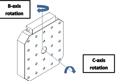
In this study, experimental tests have been done with the same set of rotary axes indexations. As mentioned before, it is better to keep all conditions constant in the different tests to have a better comparison. All the axes indexations which were used in this project are shown in figure 4-8. In these figures, there is no loading fixture and the aim is only to show the pallet in different locations. Figure 4-7 shows the position of the B and C axes.
Figure 4-7: The position of B and C rotary axes of the machine pallet
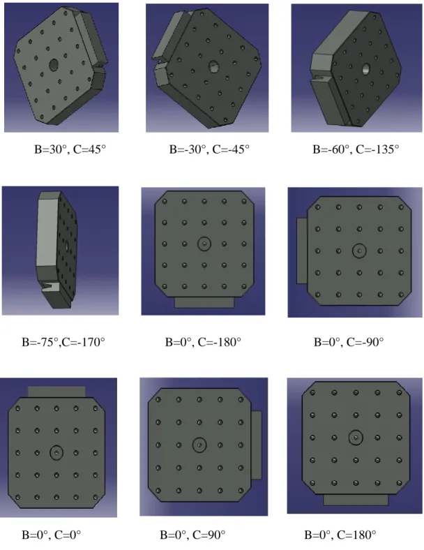
B=-90°, C=-180° B=-45°, C=-90° B=0°, C=0°
B=30°, C=45° B=-30°, C=-45° B=-60°, C=-135° B=-75°,C=-170° B=0°, C=-180° B=0°, C=-90° B=0°, C=0° B=0°, C=90° B=0°, C=180°
There are 19 combinations for each test. Figure 4-8 indicates 15 out of 19 combinations. For the last 4 combinations, The B and C axis are set to zero and the A axis (spindle rotation) are set to 0, 90, 180 and 270 degrees, respectively.
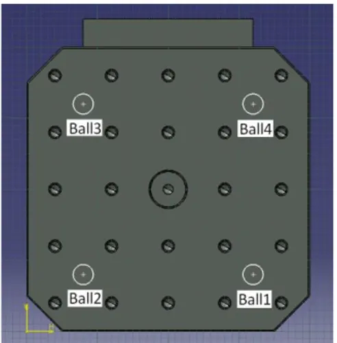
Four artefact master balls are set successively on the pallet in diagonal blocks pattern and in four corners blocks pattern. The locations in X and Y axes are constant in diagonal pattern and four corners pattern separately. This stability eliminates the result variation. The locations of master ball are shown in figure 4-9. Table 4-3 also shows the nominal master balls coordinates for all 12 tests (12 weights and torques).
Figure 4-9_a: Diagonal pattern Figure 4-9_b: 4 Corners pattern Table 4-3: The nominal master ball coordinates for different tests
The number of the test X coordinate (mm) Y coordinate (mm) Z coordinate (mm) Bar length(in) Test1 Ball1 Ball2 Ball3 Ball4 80 -80 -80 160 -80 -160 80 160 127 76.2 152.4 76.2 5 3 6 3 Test2 Ball1 Ball2 Ball3 Ball4 120 -80 -120 160 -120 -160 120 160 151.6 76.2 151.6 76.2 4 3 4 3 Test3 Ball1 Ball2 Ball3 120 -80 -120 -120 -160 120 176.2 101.6 176.2 3 4 3
Ball4 160 160 101.6 4 Test4 Ball1 Ball2 Ball3 Ball4 120 -80 -120 160 -120 -160 120 160 226.2 152.4 251.6 127 3 6 4 5 Test5 Ball1 Ball2 Ball3 Ball4 120 -80 -120 160 -120 -160 120 160 276.2 101.6 276.2 101.6 3 4 3 4 Test6 Ball1 Ball2 Ball3 Ball4 120 -80 -120 160 -120 -160 120 160 326.2 177.8 351.6 127 3 7 3 5 Test7 Ball1 Ball2 Ball3 Ball4 120 -120 -120 120 -120 -120 120 120 126.2 177 126.2 151.6 3 5 3 4 Test8 Ball1 Ball2 Ball3 Ball4 120 -120 -120 120 -120 -120 120 120 176.2 227 176.2 201.6 3 5 3 4 Test9 Ball1 Ball2 Ball3 Ball4 120 -120 -120 120 -120 -120 120 120 226.2 227 226.2 201.6 3 5 3 4 Test10 Ball1 Ball2 Ball3 Ball4 120 -80 -120 160 -120 -160 120 160 201.7 127 201.7 101.6 3 5 3 4 Test11 Ball1 Ball2 Ball3 Ball4 120 -80 -120 160 -120 -160 120 160 301.7 177.8 301.7 152.4 3 7 3 6 Test12 Ball1 Ball2 Ball3 Ball4 120 -80 -120 160 -120 -160 120 160 277.2 177.8 277.2 101.6 3 7 3 4
4.7 Validation test
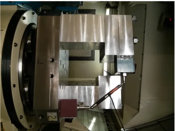
In chapter two, the maximum deflection and the angel of the deflection for different loading conditions were calculated theoretically. But it is important to validate the results with a practical test to prove that there is no significant deflection on the blocks. Thus, an experimental test was defined for verifying the deflection of the blocks on the machine. In this test, 10 blocks were mounted diagonally on the pallet of the machine. A magnetic ball bar Renishaw was then used to show the distortion of its length. One magnetic sphere was mounted on a side of the top block and the other was placed on the pallet. The Renishaw ball bar was then connected to the computer to show the exact length of the ball bar at each 5 degree of C-axis rotation. The nominal length of the ball bar was equal to 150 mm. The ball bar should be first calibrated and then placed on the machine. Figure 4-10 and figure 4-11 show the set up for validation test. Figure 4-12 presents the length variation of the ball bar for different C-axis rotations.
Figure 4-11: The validation test set up with blocks and spacers
(a) (b)
Figure 4-12: The length variation of the magnetic ball bar Renishaw, (a) with only blocks and (b) with blocks and spacers
In figure 4-12 the trends resemble a circle. This indicates that the maximum length variation of the ball bar is 2 μm. Thus, it can be concluded that the deflection of the blocks is insignificant. In the validation test, we did not calculate the deflection of the blocks directly. However, there is a possibility to verify the maximum deflection of the blocks with respect to the length variation of the magnetic ball bar. Figure 4-13 shows the 2D schematic of the validation test. Equation 4-1 presents the relationship between the maximum deflection of the ball bar and the ball bar length variation by assuming that the deflection of the blocks and the deflection of the ball bar are equal.
Figure 4-13: The 2D schematic of the validation test
́ ≅ → 𝐿 = √
+
→
=
√
= 𝜃
(4-1)As it is shown in equation 4-1, the maximum deflection of the blocks is a function of the angle (θ). Thus, the best set up for the validation tests is that the ball bar is mounted on the machine pallet parallel to the surface of the pallet (vertical). In that case, the ball bar length variation will be equal to the deflection of the ball bar (L = y).
𝑦́
𝑦
𝐿
𝜃
Chapter 5 Analyze the error data
In total, there are 26 motion errors and each error has maximum five coefficients which are called estimated error coefficients. The values of these coefficients are calculated by RUMBA method using the raw data obtained from machine tool. Thus, the polynomial function of each type of the error (motion error) can be achieved by using their coefficients.
5.1 Polynomial graphs
The polynomial function can be written as a function of one, two or more arguments. Equation 5-1 indicates the polynomial function „F‟ of „x‟ argument. In this equation, „F‟ is a polynomial function, „x‟ is argument, „n‟ is a non-negative integer and , , , … are constant coefficients.
F(x) = + + + … + + + (5-1)
The polynomial functions can have different graphs with respect to their degree. Figure 5-1 indicates the graphs of different degree of polynomial. The graph of a non-constant polynomial always tends to infinity when the variable increases indefinitely [26].
The range of motion errors can be defined as polynomial functions. Each degree of the error indicates one of its error coefficients. For instance, the polynomial function of the error EXX is defined as equation 5-2:
EXX = + + + + (5-2) EXX0 is the zero degree error coefficient which is constant and it shows the value of the EXX
regardless to volumetric errors. EXX1 is the first degree error coefficient and it indicates the linear polynomial equation of EXX. is the second degree error coefficient which shows the quadratic polynomial equation of EXX. is the third degree error coefficient and it indicates the cubic polynomial equation of EXX. is the fourth degree error coefficient (which is called backlash error) and it indicates the cubic polynomial equation of EXX.
All the other range of motion errors follows the same equation (5-2) to define their polynomial function.
Therefore, each range of motion error can be written as a polynomial function by using the values of their coefficients which have been estimated (Appendix ΙΙ). In other words, each error coefficient of each motion error is estimated by RUMBA using the raw data obtained from the machine and then entered in polynomial equation. The polynomial graphs of each motion error in different set up (experimental tests) are sketched and overlaid to show how the range of the error changes for different loading conditions. Thus, it is possible to follow the trends of each range of error with respect to different weights and torques. Plotting polynomial curves have been programmed in Matlab (Appendix Ι).
The following figures show the polynomial graphs of each range of motion error for different weights and torques. To have a better understanding of how the error changes, the rainbow colors have been used. They start with color blue and end with color red. The order of the colors is presented below and also shows graphically in Figure 5-2:
1. Blue continues : test1 (W=0N, T=0N/m) 2. Blue dash : test2 (W=200N, T=5N/m)
3. Cyan continues : test10 (W=200N, T=20N/m) 4. Cyan dash : test12 (W=200N, T=35.2N/m)
5. Green continues : test7 (W=400N, T=10N/m) 6. Green dash : test3 (W=400N, T=20N/m) 7. Yellow continues : test4 (W=600N, T=45N/m) 8. Yellow dash : test11 (W=600N, T=90N/m) 9. Magenta continues : test8 (W=800N, T=40N/m) 10. Magenta dash : test5 (W=800N, T=80N/m) 11. Red continues : test9 (W=1000N, T=75N/m) 12. Red dash : test6 (W=1000N, T=125N/m)
Figure 5-2: The rainbow colors of the polynomial graphs
In these figures, the horizontal axis shows the range of the corresponding joint positioning. These ranges can be defined from the probing file. To this aim, the maximum and the minimum values of each axis should be considered.
The range of the X axis is equal to [-300 mm, 300 mm]. The range of the Y axis is equal to [-250 mm, 250 mm]. The range of the Z axis is equal to [0 mm, 305 mm].
The range of the A, B and C axes are equal to [0°, 360°], [-90°, 90°] and [-180°, 180°] respectively. 0 20 40 60 80 100 120 140 0 200 400 600 800 1000 1200 To rq u e (N /m ) Weight (N)
EXX = + + + +
Figure 5-3: The polynomial graphs of the error EXX
At X equal to zero there is no EXX error. In other words, when the machine pallet doesn‟t move in X direction, the EXX error is zero; but as soon as the pallet moves in X, the EXX error will be created.
The graphs are quite similar which have ascending trajectory in large weights and torques and descending trajectory in small values of weights and torques. If we follow the colors from color blue to color red, the value of the error generally decreases by adding more load on the machine. The absolute value of the error in each graph is symmetrical and that is expected. The maximum error value is around 0.2 mm and the minimum absolute value is 0 mm.
EYX = + + + +
Figure 5-4: The polynomial graphs of the error EYX
There is no EYX error at X=0mm. It means that the value of the error is equal to zero or the effect of load neutralized this type of motion error at X equal to zero.
Some of the graphs have ascending trajectory and some other have descending trajectory in different loading conditions.
From color blue to color red, the value of the error generally increases by increasing weight and torque.
EZX = + + + +
Figure 5-5: The polynomial graphs of the error EZX
There is no EZX error at X=0mm. It means that the value of the error is equal to zero or the effect of load neutralized this type of motion error at X equal to zero.
Most of the graphs have an ascending trajectory in the range of X axis. In other words, when the machine pallet moves from X ( ) to X (+), the value of the EZX motion error will increase. From color blue to color red, the error value generally decreases by adding more load on the machine.
EAX = + + + +
Figure 5-6: The polynomial graphs of the error EAX
If we follow the colors from color blue to color red (which belong to minimum weight and torque and maximum weight and torque respectively), the value of the error generally increases by adding more load on the machine.
The trends of the graphs are quite constant in the range of the X axis position. It means that the value of the EAX error doesn‟t change significantly from X ( ) to X (+).
The maximum absolute value of the error is close to 0.001 mm and the minimum absolute value is 0.
EBX = + + + +
Figure 5-7: The polynomial graphs of the error EBX
There is no EYX error at X=0mm. It means that the value of the error is equal to zero or the effect of load neutralized this type of motion error at X equal to zero.
The value of the error in the range of positive X is larger than the error value in the range of negative X.
The value of the EBX motion error doesn‟t change significantly by adding more load on the machine. Thus, it can be concluded that adding load on the machine doesn‟t affect this type of motion error significantly.
ECX = + + + +
Figure 5-8: The polynomial graphs of the error ECX
The trends of the graphs are quite constant in the range of the X axis position. It means that the value of the ECX error doesn‟t change significantly from X ( ) to X (+).
From color blue to color red, the error value generally increases by adding more load on the machine.
EXY = + + + +
Figure 5-9: The polynomial graphs of the error EXY
If we follow the colors from color blue to color red (which belong to minimum weight and torque and maximum weight and torque respectively), the value of the error generally increases by adding more load on the machine.
All the graphs follow the same trend in the range of Y axis. They have a completely ascending trajectory according to the absolute values.
The maximum absolute error value is around 0.33 mm and the minimum absolute value is close to 0.12 mm.
EYY = + + + +
Figure 5-10: The polynomial graphs of the error EYY
The value of the error increases from negative Y to positive Y.
From color blue to color red, the error value generally increases by adding more load on the machine.
Most of the graphs have similar trend (quite constant in the range of Y axis). However, some graphs such as cyan continues, cyan dash and yellow dash have different patterns.
EZY = + + + +
Figure 5-11: The polynomial graphs of the error EZY
There is no EZY error at Y=0mm. It means that the value of the error is equal to zero or the effect of load neutralized this type of motion error at Y equal to zero.
Most of the graphs have the same trend which is quadratic. It means that the EZY motion error is symmetric in the range of Y axis.
From color blue to color red, the error value generally decreases by adding more load on the machine.
The maximum absolute error value is close to 0.055 mm.
EXZ = + + + +
Figure 5-12: The polynomial graphs of the error EXZ
There is no EXZ error at Z=0mm. It means that the value of the error is equal to zero or the effect of load neutralized this type of motion error at Z equal to zero.
All the graphs have ascending trajectory in the range of Z axis position. In other words, the error values increase by increasing the value of Z axis.
From color blue to color red, the error value generally increases by adding more load on the machine.
EYZ = + + + +
Figure 5-13: The polynomial graphs of the error EYZ
Most of the graphs have the same trend. However, some graphs (magenta dash and yellow dash) have different trajectory.
There is no EYZ error at Z=0mm. It means that the value of the error is equal to zero or the effect of load neutralized this type of motion error at Z equal to zero.
Adding more loads on the machine pallet doesn‟t have any significant effect on the error values. The maximum error value is close to 0.07 mm.
EZZ = + + + +
Figure 5-14: The polynomial graphs of the error EZZ
There is no EZZ error at Z=0mm. It means that the value of the error is equal to zero or the effect of load neutralized this type of motion error at Z equal to zero.
The range of the error value in large weights and torques are quite constant in Z axis position. If we follow the colors from color blue to color red (which belong to minimum weight and torque and maximum weight and torque respectively), the value of the error generally decreases by adding more load on the machine.
EAZ = + + + +
Figure 5-15: The polynomial graphs of the error EAZ
The values of the error in small weights and torques at Z equal to zero are insignificant, but in large weights, they start from -0.0006 mm.
The error values generally decrease in the range of Z axis. In other words, when the probe moves forward to approach the master balls artifact, the EAZ value will decrease.
ECZ = + + + +
Figure 5-16: The polynomial graphs of the error ECZ
Most of the graphs (except magenta dash and green continues) have the same trend and their value is close to zero in the range of Z axis position.
Adding more loads on the machine pallet doesn‟t have any specific effect on the error value in most of the loading conditions.
EXB = + + + +
Figure 5-17: The polynomial graphs of the error EXB
All the graphs have an ascending trajectory (except magenta dash) in the range of B axis. In other words, the absolute error values generally decreases from B= -90°to B= 90°.
The graphs are quite close to each other in the range of B axis. It means that adding more loads on the machine doesn‟t have significant effect on the EXB error value.
EYB = + + + +
Figure 5-18: The polynomial graphs of the error EYB
All the graphs have the same trend. From color blue to color red, the error value generally increases by adding more load on the machine.
The absolute values of the error decrease in B negative and increase in B positive in most loading conditions.
Magenta dash which belongs to test number 5 (W=800N, T=80N/m) changes much more than the other graphs in the range of B axis.
EZB = + + + +
Figure 5-19: The polynomial graphs of the error EZB
Most of the graphs have the same trend except red dash which belongs to maximum weight and maximum torque.
The graphs are quite close to each other in the range of B axis. It means that adding more loads on the machine doesn‟t have significant effect on the EXB error value.