Design of a gas force simulator for the MIT Electromechanical Valve Drive project

Design of a Gas Force Simulator for the MIT Electromechanical Valve Drive

Project

By

James S. Otten

SUBMITTED TO THE DEPARTMENT OF MECHANICAL ENGINEERING IN

PARTIAL FULFILLMENT OF THE REQUIREMENTS FOR THE DEGREE OF

BACHELOR OF SCIENCE

AT THE

MASSACHUSETTS INSTITUTE OF TECHNOLOGY

JUNE 2006

©2006 James S. Otten. All rights reserved.

Thr i

t r

+li

Urf.h-,1

-r

,

n MT

An

n-rm irn

+-

r

llr

MASSACHUS OF TEC

AUG I

LIBR

I I., aulul I 11i.. wIJ uy Ia1L L 1V1 YJ,111LUll L. I.IJIUiU.-.

-and to distribute publicly paper -and electronic copies of this thesis document in whole or in part

in any medium now known or hereafter created.

Signature of Author:

, /.

Department of Mechanical Engineering

May 12, 2006 Certified by:

Accepted by: A.

Thomas A. Keim

___..II __

Principal Research Engineer

Thesis Supervisor

,

_-- x

z

John H. Lienhard V

Professor of Mechanical Engineering

Chairman, Undergraduate Thesis Committee

SETTS INSTITUTE ,HNOLOGY 2 2006

ARIES

-Design of a Gas Force Simulator for the MIT Electromechanical Valve Drive

Project

by

James S. Otten

Submitted to the Department of Mechanical Engineering

on May 12, 2006 in Partial Fulfillment

of the Requirements for the Degree of

Bachelor of Science in Mechanical Engineering

Abstract

The MIT electromechanical Valve Drive (EMVD) is a continuously variable valve actuation device for an automotive internal combustion engine. Current experimentation of the EMVD has been limited to intake valve events. When the exhaust valve opens into the cylinder it must do so against gas forces arising from high pressure in the engine cylinder. This gas force causes power losses in the EMVD. A gas force simulator has been designed to simulate the pressure acting against the exhaust valve in the engine cylinder. This allows the power loss as a result of the gas force to be

measured for the EMVD.

1.0 Introduction

The cycle of an automotive internal combustion engine requires that gases are

exchanged between the engine intake and exhaust manifold and the combustion chamber.

Valves are used to control the flow of these gas exchanges. Conventional automotive

valves are opened and closed using a cam system attached to a camshaft. The camshaft is connected to the crankshaft of the engine by either a chain or a toothed belt. In

conventional systems the length of the chain or toothed belt does not change with respect

to time. Therefore the camshaft and cam profile are fixed relative to engine crank angle.

Pure optimization of valve timing can only occur at a specific engine speed and

throttle position. This leads to decreased efficiency or performance in the ranges of

operating conditions where the system is not optimized. Variable valve timing allows the

valves to be opened and closed at different crank angles as operating conditions change.

Most systems currently employed on production vehicles include variable valve

timing. A hydraulic cam phaser is used to vary the cam timing with respect to engine crank angle. The profile for these systems, however, is fixed, and so lift and opening

duration cannot be varied according to engine operating conditions.

The MIT Electro-Mechanical Valve Drive (EMVD) is a continuously variable valve timing actuation system. It uses an electrical servo motor to drive a cam. The servo motor is driven through an electrical signal and is not driven directly coupled to the engine crankshaft speed. This allows the valve timing to be optimized at all engine speeds and leads to increased engine efficiency. The EMVD employs a non-linear

mechanical transformer that is optimized for fast transition times, lower power

consumption, and low seating velocities.

Current experimental results for the EMVD are only applicable to the intake valve

process. The experiment is set up on a test bench with a valve that opens from a valve seat to the environment. During the engine intake process there is little pressure

difference between the intake manifold and the combustion chamber above the piston.

For this reason there is no net force from gas pressure against the valve. It is therefore accurate to simulate this process with a valve opening into free space as is done on the current experimental setup.

To realize the full benefits of continuously variable valve timing, the system must be installed on the exhaust valves as well as the intake valves. Besides differences in valve geometry there is also gas pressure acting against the valve face during the exhaust process. Residual pressure from the combustion process causes a large pressure drop to occur across the valve. This pressure differential leads to a net force that acts against the opening of the valve. As the valve opens into the combustion chamber the pressure in the cylinder is released. During this process, the retarding gas force causes power losses in the system that are not present in the intake process.

The combustion process is a fairly well understood event. The pressure as a function of time has been well studied experimentally. A simulation could be used to predict the power loss that occurs when the EMVD valve opens. Experimental results could differ from the predicted response due to the differences in valve opening procedure seen in the EMVD as opposed to a valve system of conventional design.

An experimental apparatus has been designed to simulate the gas force acting against the valve. The valve opens into a pre-pressurized chamber simulating the

combustion chamber. As the valve transitions from closed to open the pressure is released. By measuring the input power to the motor while opening the valve against the gas pressure, a measure of the power consumption of the system can be made.

2.0 Experimental Approach

In order to experimentally measure the power loss incurred by the gas force acting against the valve, a force versus time profile must be simulated. Several methods of simulating the gas force acting against the valve opening event were evaluated in the

process of obtaining a suitable method for simulation.

The data used for this project was obtained from a digital computer simulation of

a cylinder combustion event. The simulation has been developed by Prof. Wai K. Cheng

of MIT's Sloan Automotive Lab and is known to correlate well with experimental

measurements. The engine simulation provided cylinder pressure, temperature and other

engine parameters as a function of engine crank angle. The results of the engine

simulation are provided in Appendix A. From this engine simulation a suitable model of

the gas force versus time could be determined.

An alternative approach to cylinder pressure data would have been to obtain data

for the force acting against the valve itself. This approach would have required the use of strain gauge instrumentation. A strain gauge would need to be fixed on the valve or cam

itself during the engine run cycle. While not impossible, this type of data would be very

hard to obtain experimentally. Data of this form was not obtainable for the purposes of

this experiment.

The best source of data for comparison was provided in the form of a cylinder pressure profile. Due to the availability of the cylinder pressure data, the pressure in the cylinder was chosen as the primary variable to simulate with the proposed experiment.

Using the gas force coefficient as described in the theory section it is possible to extract an estimation of the gas force acting on the valve. With gas force reference data and the cylinder pressure, several options were explored to obtain the most effective

solution.

The approaches to the question of simulation come in two distinct ways: pressure

simulation and force simulation. Pressure simulation describes those simulators which

would engage the valve through pressure acting on it, the same way it is acted on in an automobile engine. Force simulation describes those simulators which use mechanical means to apply a force directly through the valve without traveling through a fluid medium.

2.1 Force Actuation

Several force simulators were evaluated. Among the force simulators, the two most prominent were hydraulic and electromagnetic force actuators. The relatively high forces required, relative to transition speed, dictated a strong actuator be used in the

experiment. Hydraulic actuators were proposed because of their high force density

capability but were rejected because of their extremely slow speed when compared to

valve transition speed.

Electromagnetic actuators showed initial promise as their force capabilities are in line with those required for the gas force. With any moving actuator comes the question of inertia and this is the failure with regards to electromagnetic actuation. The force profile needed is quite linear and decreases with time. Without the use of complex linkages it is difficult to approximate linear motion with a rotary actuator. This leaves

linear motors as a possibility. Linear motors are quite expensive as they are a relatively

new technology. Also problematic with linear actuators are their force to inertia ratios.

To follow the acceleration of the valve transition, an inertial mass of 100 g would require a force equal to the desired valve force. This dictates that the armature and any other moving components of a linear motor be well below this value so that the force required for the actuator to move itself not be dominant over the force applied to the valve. A

review of "off the shelf' linear actuators revealed the improbability of obtaining an

actuator that would fulfill the necessary characteristics.

2.2 Pressure Actuation

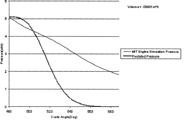
An experimental apparatus that simulates force through pressure was also considered. The simplest and easiest approach would be to simply create a volume of

pressure that could act on the valve face. The volume would contain an initial pressure

equal to that of the pressure in the engine cylinder at Exhaust Valve Opening (EVO).

This volume would then be exhausted through the orifice between the valve and the valve

seat. This style of apparatus leaves only the volume of the cylinder as the variable with

which to tune the time constant to match that of the actual engine pressure profile.

Results of such a simulation are shown in Figure 1.

4 M ~3 tii `' 0. 0 2₁ 0 Volume = .001 mrA3

- MIT Engine Simulation Pressure

I Predioted Pressure

483 503 623 543 C rark Angle(D eg)

63 5683

Figure 1 Simulated Pressure Vs. Engine Cylinder Pressure for Single Opening Event

In such an apparatus the only orifice for gas to be exhausted through is the valve itself. A

mass flow rate out of the orifice. Therefore, the only way to control the rate of pressure

loss in the tank is to vary the initial volume of the cylinder. Because of the slow opening velocity of the EMVD valve, the rate of pressure decrease in the simulator cylinder, during the first 30 degrees of crank angle, is not sufficient to equal the rate of pressure decrease in the engine cylinder. The initial flow through the valve is zero and so the rate

of pressure decrease as a function of time is initially zero. The initial rate of pressure

decrease in the engine cylinder at EVO is non-zero and so no single orifice that opens at EVO will be able to simulate the pressure in the engine cylinder during the initial opening stages.

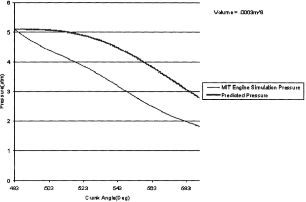
The best possible simulation for this type of apparatus is one in which the rate of

pressure decrease is approximately equal to that of the engine simulation. However, when

this situation occurs, it occurs with a time offset as shown in Figure 2.

5 4 3 0. 2 1 0 Volum e = .O003m'3

-_ MIT Engine Simulation Pressure

N P, redicted Pressure l

483 503 523 543 583 583

C rark Angle(D eg)

Figure 2

For this reason it will not give an accurate measure of the power loss during the

blow down event.

A choked flow orifice gives a reasonably linear rate of flow. This leads to a linear

pressure decrease as a function of time which is what occurs in the engine cylinder.

Since a linear rate cannot be achieved with the single valve orifice, a device including a second orifice was devised. The second orifice would be large with respect to the valve orifice in an effort to achieve the desired pressure versus time profile. The secondary orifice would be opened at a predetermined time before the opening of the primary valve so that the choked flow could be fully developed. The necessary dimensions of the volume and orifice size present modeling issues. The quasi-static model assumes a small

orifice size relative to volume. The necessary dimensions for a secondary orifice dictate that the orifice be almost the same diameter as the tank diameter. In a case such as this

where the quasi-static model breaks down, flow geometry and unsteady compressible

flow models must be utilized to obtain an accurate representation. This type of analysis

is best suited for Computational Fluid Dynamics (CFD). The time intensive nature of

CFD analysis made it an unattractive alternative for the purposes of this experiment.

Another option in pressure simulation was to explore the use of a moving

boundary. It was thought that a moving boundary such as the piston and cylinder in an

automobile engine might better represent the pressure profile. The transition time for the EMVD is approximately 3ms which correlates to 108 deg of crank angle in an engine running at 6000rpm. In an actual engine the 108 degrees of crank angle means that the

piston reverses direction at some point during the exhaust valve opening event. This

however is only a part of the complex combustion occurring during the event and so the

pressure in the cylinder is actually a steady decrease due to the combination of moving

piston, residual burning and other factors.

In creating a moving boundary model, practical apparatus issues were considered.

Because of the short duration of the event it would be difficult to create a system that was initiated from rest as the valve event was beginning to occur. The inertia of any moving

boundary would make it nearly impossible and so reciprocating applications were of

primary focus.

In order to investigate the possibility of using a reciprocating moving boundary a

quasi-static model was used. It used the simulation of the valve opening and the flow out

of the orifice as a baseline. From there a script was run to produce the optimal volume in a chamber to achieve the exact values shown in the simulation. The necessary volume profile is shown in Figure 3:

0.007 0.006 0.006 E 0.003 0.0231 0.001 0 480 500 520 540 50B 580 Crank Angle(deg)

Figure 3 Ideal Volume for a non-static Volume

The linearity of the curve makes it difficult to approximate with a reciprocating piston. It

was determined from the model that in order to best approximate the curve, a large bore and stroke would be needed. This however makes physical implementation difficult as the necessary bore size was 3 inches with a 4.5 inch stroke. This severely limited the choices for piston cylinders. It was for this practical reason that this option was eventually abandoned in favor of another use of the static cylinder approach. 2.3 Staged Static Cylinder

Of the possible designs for gas force simulation, no single stage design satisfies

the requirements for simulation experimentation. No design is suitable for either

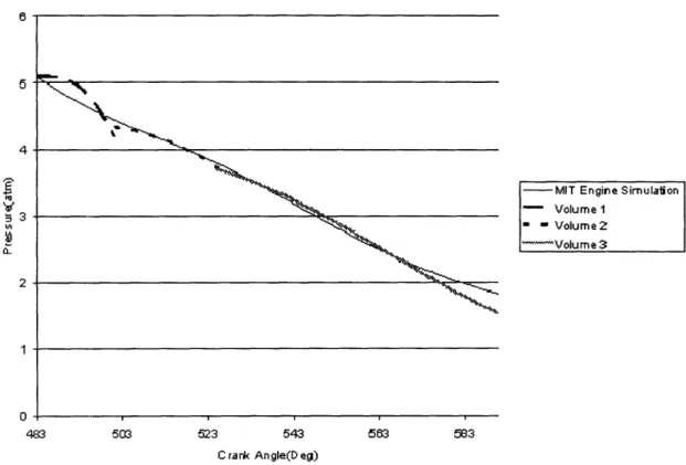
simulation or fabrication. The simplest choice also provides the most flexibility. A multi staged event could be used to obtain a measure of the valves power loss. Multiple

volumes could be used to approximate different times during the valve event. Volume and initial pressure could be varied to obtain the desired response. This solution is not the most elegant, but will provide a reasonable idea of the power loss before the valve is implemented into an actual engine.

The more stages in the experiment the better the approximations can be. A plot displaying several stages overlaid on top of each other is shown below.

MIT Engine Sirnulation

- Volume 1

- - Volume2

Volu m e 3

503 523 5463583 83

C rank Angle(D eg)

Figure 4

6 4 3 a 2 0 483

3.0 Theoretical Background

The theoretical model used to simulate the pressure as a function of time in the simulator is based on the choked mass flow equation. The gas force simulator is modeled as a large pressure vessel with a small orifice open to the atmosphere. The size of the

orifice is small with respect to the volume of the container so a quasi-static model is used

to describe the state of the vessel. An assumption is made that the mass flow out of the

cylinder is always under the choked flow condition. The model makes no effort to

describe the developing flow region.

The model begins with the mass flow out of the cylinder. The mass flow rate out

of the cylinder is governed by the choked flow rate equation for critical pressure ratios in

excess of .528. The critical pressure ratio is defined as the ration of the upstream

pressure to downstream pressure. Since the initial pressure for the EVO event is 75psi, the equation applies. The governing choked mass flow rate is shown below:

Q C

P

2

( r+)/(r-l)

Q

=

CAikp(

I)

(1)

where Q is the mass flow rate out, A is the orifice cross sectional area, y is the ratio of the specific heat, p is the density of the gas in the cylinder, C is the flow coefficient and P is the pressure in the cylinder. The state of the gas in the cylinder is modeled using the ideal gas law:

PV = mRT

(2)

where V is the volume of gas in the cylinder, m is the mass of the gas in the cylinder, R is the universal gas constant, and T is the temperature of gas in the cylinder.

The temperature of the gas in the cylinder is found as a function of the mass of the gas in the cylinder using the following derivation.

The change in the total energy of the control volume E, can be written as a function of the mass flow mr and the enthalpy h entering and exiting the control volume.

dEcv

= rhi - rhho.. (3)

dt

Since the pressure in the control volume is greater than 1 atmosphere, no mass flows into

the control volume.

Mhin =0 (4)

Therefore the change in energy in the control volume is only a function of the mass flow

out of the control volume.

Ecv=

_{= -mht}

₍₅₎

dt out

The energy in the control volume can be expressed as a function of the mass in the

control volume m, the specific heat at constant volume c and the temperature of the

mass in the control volume T.

Enthalpy is defined as the product of the Temperature and the specific heat at constant

pressure.

h = cT

(7)

Substituting the definition of control volume energy and the definition of enthalpy into

equation 5 yields:

d(mcT) -

cT

(8)

dt

Separating terms and rearranging gives:

dm

dT

dt

_{dt -outcpT}

Since the universal gas constant R can be related to cp and c, by:

R = cp -cv (10)

and recognizing that

dm

= -rmu

(11)

dt out

Equation 9 can be simplified to:

dT

mcV, = -m RT

(12)

dt out

Separating terms and integrating with respect to temperature and mass respectively

yields:

dT 1 m 1 dmc

₍₁₃₎

Tdt R

T m

cmcv dt

--

1

C2

1

n(m2)

(14)

T·~

Cv, m,

Rearranging terms yields:

R

k, ml J(15)

Equation 13 is used in conjunction with the ideal gas law, equation 2, to describe the full state of the gas in the control volume. For each time step the mass flow rate is calculated based on the EMVD valve displacement and the flow rate over the time step is subtracted from the total mass. This process is repeated iteratively for all time steps and the duration of the event. This process gives the mean pressure in the cylinder as a function of time for the duration of the event.

Mean cylinder pressure does not completely describe the situation during an

exhaust event. A first order model for the gas force acting against the valve F would be to simply multiply the mean cylinder pressure P and by the valve head area A.

This simple model only describes the situation before the valve has begun to open. When

the valve is closed, the cylinder head and valve can be treated as one body and so the

force over a given area can be described by the equation above. As soon as the valve

begins to open, a pressure difference across the valve is developed. The pressure in the

exhaust manifold behind the valve is taken to be approximately atmospheric. However,

once a pressure difference is established and flow develops in the gap between the valve

and the valve seat, the pressure on the back side of the valve changes. The flow is

accelerated by the pressure difference across the valve. The pressure in this region of

high velocity is lower than the cylinder pressure but still greater than atmospheric. A

complete description of the fluid dynamics involved requires an in depth study using

Computation Fluid Dynamics (CFD)

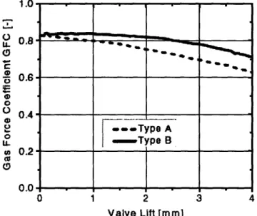
The flow effects during the valve transition can be described by using a lumped

parameter coefficient. The Gas Force Coefficient (GFC) is the ratio of the gas force as predicted by a CFD model to the gas force as predicted using the simple model of the pressure difference. The GFC is plotted for a representative valve in Figure 5.

4 n_ . I .U' O0.8

u-0

nn

Figure 5 Gas Force Coefficient During Exhaust Valve Opening'

The curve represented by Type A in the figure above shows the GFC for representative valve and valve seat geometry. Type B represents a unique CFD optimized valve. For the purposes of this experiment a valve similar to the geometry in Type A was used for analysis purposes. The GFC is used when computing the force versus time profile for the EVO event from the pressure profile in the cylinder.

1 C. Schernus, F. van der Staay, H. Janssen, J. Neumeister, B. Vogt, L. Donce, I.

Estlimbaum, E. Nicole and C. Maerky (2002) "Modeling of Exhaust Valve Opening

in a Camless Engine" Modeling of SI Engines and Multi-Dimensional Engine Modeling

(2002-01-0376); SAE TECHNICAL PAPER SERIES

| .. Type A Type B I ^L00 ml f tm.._ L I I I I - t M'.4 . .. ... .. -Q**Lccc c .. 0,~ I ;. T r I

4.0 Experimental Apparatus

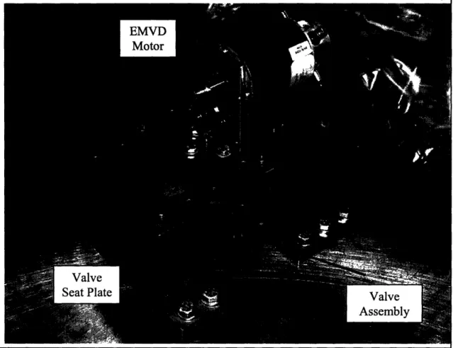
The EMVD experimental apparatus is designed to provide a rigid platform for the valve opening experiment. The apparatus is bolted to two large steel blocks which are in

turn bolted directly to a large steel table which is /2" thick. The EMVD motor is

mounted to one of the steel blocks as shown in Figure 6. In between the two steel blocks

is mounted the valve assembly. Below the valve assembly and bolted to the steel blocks is the valve seat plate. To install the gas force simulator the EMVD apparatus remains largely unchanged above the valve seat plate. The EMVD apparatus without the gas force simulator can be seen in Figure 6.

Figure 6

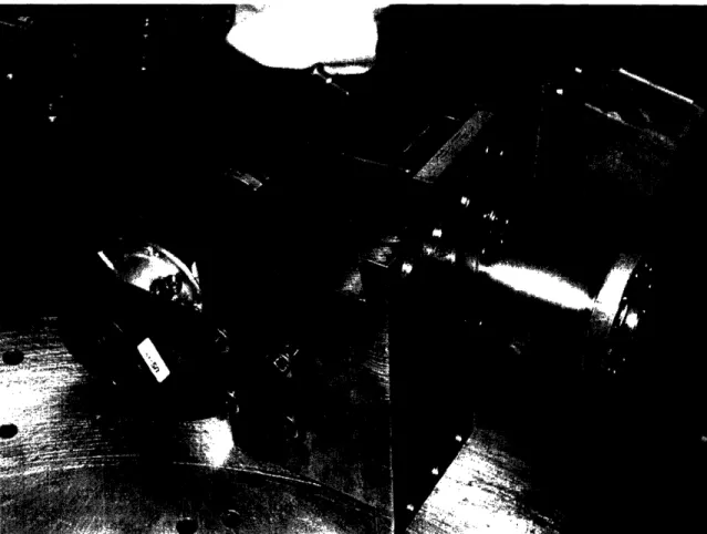
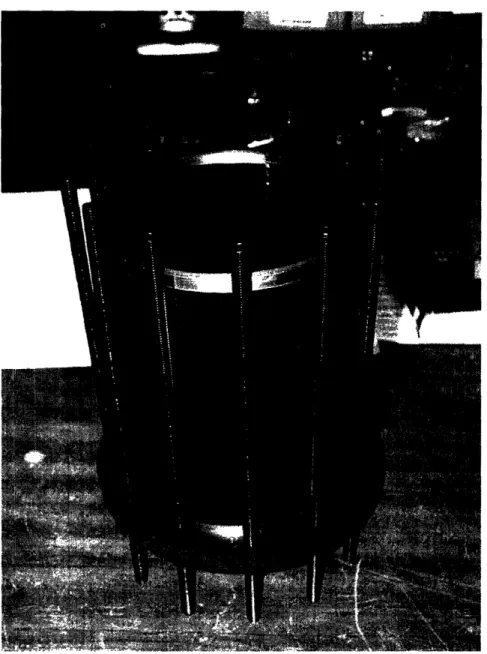
The gas force simulator consists of two separate but connected pressure vessels; a lower tank and an upper tank. In order to accommodate the connection between the tank and the valve assembly, a large hole was cut in the steel table. This was done so that the upper tank could pass through the table and be attached to the valve seat plate. The lower tank passing through the hole in the steel table is shown in Figure 7

Figure 7 Upper Vessel passing through hole in steel table

The other modification to the existing EMVD assembly was the fabrication of a new valve seat plate. The existing plate was ¼/4" thick and had several holes drilled for sensor mounting points. The new valve seat was /2" thick and not only contained the valve seat but also mounting holes for the upper tank. The plate was made from thicker material in order to provide more thread engagement for the upper tank fasteners. The upper tank extended from the valve seat plate down through the table. An o-ring was used for sealing between the upper tank and the valve seat plate and the upper and lower tanks. The lower tank connected to the upper tank with the same method as the valve seat plate. The upper tank was constructed of a tube welded with two flanges used for the mounting and o-ring grooves. The entire gas force simulator apparatus as attached to the EMVD can be, seen in figure 8

Figure 8 Gas Force simulator as attached to EMVD Apparatus

The lower tank was of large radius and was designed to be changed out without removing the upper tank from the EMVD apparatus. The upper tank was comprised of a lower and upper end plate and a tube connecting them in the middle. Unlike the upper tank the lower pieces were not welded but were retained by threaded rod that ran the length of the tank. A groove was cut into both the upper and lower plates so that the middle tube could be inserted into them. This not only provided alignment between the tube and the plates but also gave added strength to the interface where high stress concentrations exist. Into the groove was cut an additional o-ring groove. A compressor was attached to the lower pressure vessel to pre-charge the cylinders before an experiment.

because of its good weld ability characteristics as well as higher strength. The pressure

vessels were tested at 120 psig with no signs of leakage or yielding.

3.1 Procedure for Installation of Gas Force Simulator

The first step in installation is the removal of the existing valve seat from the EMVD. This process is outlined in Dr. Woo Sok Chang's Thesis2. The valve apparatus is then assembled using the gas force simulator valve seat. When installing the valve

apparatus the valve seat must be centered on the valve itself. This is done by attaching

the valve assembly to the steel motor support blocks with the four hex head bolts. The

valve should be in the neutral position at this point. With the top plate installed, the

bottom plate is free to move since the bolt holes have been clearanced to allow for

misalignment. At this point the valve is closed and the valve seat centered. With the

valve seat centered by the closed valve the plate is attached to the motor support blocks

with four hex head bolts. The Upper pressure vessel is now ready for installation.

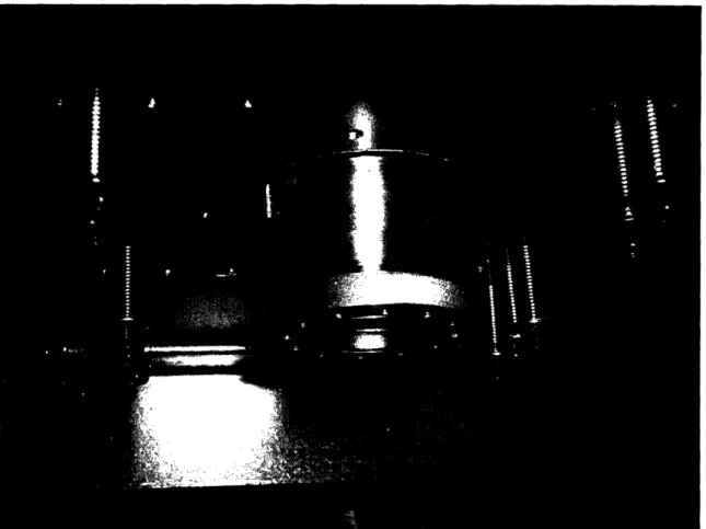
To install the upper pressure vessel, place the EMVD assembly on its side with the valve exposed. Install the pressure gauge in the upper vessel through the port and ensure that the wires do not interfere with the blocks. Place an o-ring in the groove on the top of the upper vessel and bolt in place to the valve seat. Though there are 12 holes only 6 need be used to install the vessel. The assembly at this point should be the same as shown in Figure 9.

2 Chang, Woo Sok. "An Electromechanical Valve Drive Incorporating a Nonlinear

Figure 9 Assembly picture for Gas Force Simulator

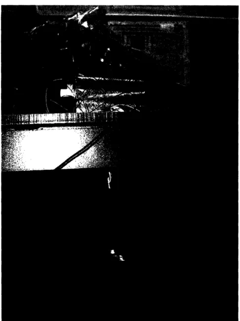
Next the assembly is flipped upright and the upper vessel passed through the hole in the table. The top of the lower pressure vessel is then installed on the upper vessel. An o-ring is placed on the bottom of the upper pressure vessel and the upper piece of the lower vessel is bolted in place. The remainder of the Gas Force Simulator can be installed on the bench prior to being installed in the table. The tube and lower end plate are

assembled with an o-ring seated in the groove in between. Threaded rod is passed through the holes as is shown in Figure 10.

Figure 10

With the lower section assembled it can now be fitted to the upper end plate. An o-ring must be installed in the groove in the upper end plate. This is particularly difficult because the groove is inverted. One solution is to use grease rubbed on the o-ring to adhere it to the groove long enough to install the tube section. Once the tube is fitted and the threaded rods passed through the upper end plate, nuts are used to attach the three sections. Lastly the 3/8NPT pressure fittings used to supply the tank are fitted into the bottom of the lower vessel plate. Tubes can be run from the Gas force Simulator to any local air supply. This completes the assembly. A figure of the assembled gas force simulator and valve seat plate without being attached to the EMVD is shown in Figure 11

5.0 Experimental Procedure

The EMVD is controlled via the lab computer for the duration of this experiment.

The pressure sensor on the gas force simulator is connected to the computer via a bridge

amplifier. The position of the EMVD motor is measured through a position sensor

attached to the armature of the motor. A current sensor is also placed on the motor power

supply to measure current driving the motor.

To run the experiment, the gas force simulator must be prepared for an Exhaust

Valve Opening (EVO) event. The EMVD valve is moved to the closed position. The

closed position not only brings the valve to its start position, but also allows for sealing

between the valve and the valve seat. This allows the gas force simulator to be pressurized to its predetermined value. Once the valve is in the closed position the external compressor tank is charged to the intended initial pressure for the EVO event. To simulate the highest opening pressure the simulator pressure is raised to 75 psig. The

valve is opened and the simulator is allowed to reach equilibrium with the external tank.

The flow rate into the simulator is less than the leakage rate past the valve and so the external tank compressor can bring the simulator to pressures in excess of 120 psig. This is well above the maximum pressure seen at the valve during the actual engine EVO event. A digital multimeter is connected to the bridge amplifier on the pressure gauge so

that an accurate reading of the pressure can be used to pressurize the tank. Once the

pressure in the simulator has equilibrated and the desired initial pressure reached, the experiment is ready to be performed.

The actual experiment is performed by opening the EMVD valve. As it is opened, the pressure in the gas force simulator is released through the valve orifice into

the atmosphere. Once the valve has been opened, the event is complete and the data

recorded. The compressor is not disconnected from the simulator before the event is performed. The leakage rate through the valve in the closed position dictates that in order

to maintain a constant pressure in the simulator prior to the event, the compressor must

continue to supply a flow rate. This mass flow rate into the cylinder during EVO is

negligible compared to the flow rate out of the cylinder.

This procedure is run for 5 different initial starting pressures. This was done to

test the valve and ensure that the valve was capable of opening against the back pressure

6.0 Results

Five Exhaust Valve Opening (EVO) events were conducted.

conducted at 30,45,60,75, and 90 psig for initial pressures before EVO.

one such event, conducted at 30psig are shown in

below.

j

-'3

It !

I i

I"

I i

_I

_r

_f

I

_IL

_a

/

-

_W

The results of

Figure 12 Pressure, Valve Position, and Current for 30psig EVO event.

The current to drive the motor for this experiment was limited to 15 amps. The motor

controller was run open loop as exhibited by the step input of current to the motor as shown in Figure 12 above. The current to the motor is regulated by an MIT fabricated

dc-dc converter with internal switching at approximately 80kHz. This converter has

relatively large electromagnetic emissions which are observed to substantially contaminate the output of the pressure sensor amplifier. As a result, accurate pressure measurements during the actual test event were unobtainable. Several methods of

isolation were attempted to obtain pressure readings during the event but none were

successful. Despite the lack of data during the event, pressure measurements after the event were obtained and the exponential decay of the system can be seen above. During this test, the motor did not complete a full transition and so oscillated about the neutral spring position after the event as shown in the figure. With the current limit set to 15A the EMVD was unable to complete a full transition against 30psig of back pressure.

The EMVD was run during the experiment with an open loop controller. The controller was designed to minimize power loss, transition time, and seat velocity for an

I· · I I II r Ad

I I II I I

A

hoped that if a new control scheme, optimized to handle the exhaust back pressure could

be developed, that it would be able to open the valve against the back pressure.

Measurements were taken for EVO events at six different initial pressures. The

pressure for each of these events is plotted as a function of time in Figure 13.

100 90 g0 70 a, a 50 40 30 20 10 0 0 0.05 0.1 0.15 0.2 0.25 0.3 Times)

Figure 13 Measured Pressure vs. Time for 5 EVO events

The pressure data taken was quite noisy due to the close proximity of the dc-dc converter to the pressure gauge and amplifier and the nature of the pressure gauge itself. The data presented in the figure above is an average taken every 100 data points. The initial noise that was not filtered was due to the high current input to the motor during the event. After the event for all of the pressure curves, a linear region is apparent. The linear region extends from the initial opening pressure down to approximately 25 psig though it varies somewhat between the curves. After the linear region the systems exhibits an exponential decay and finally equilibrates with the atmosphere at Opsig. Data from the 90psig event is shown in Figure 14. Only the linear region is shown to obtain the

pressure rate during this linear flow region

-- 100 per. Mov. Avg. (90 psi Pressu re)

... 100 per. Mov. Avg.

(75 psi Pressu re)

- 100 per. Mov. Avg.

(45 psi Pressu re)

.100 per. Mov. Avg.

(30 psi Pressu re)

--- - 100 per. Mov. Avg.

90 80 70 '. 50 Y.U 2 40 30 20 10 0 y = -10.71x+ 91 .O9 ---- Pressure Linear (P ressu re)

0.04 0.05 0.07

Time(s)

O.0O 0.09 0.1

Figure 14

A linear best fit line has been applied to the pressure data to obtain an approximate pressure decay rate of 51 Opsig/s. Data obtained from the four other events can be found in Appendix B.

7.0 Discussion

The pressure profiles obtained from the five EVO events had mixed results. The

pressures measured followed the general model for the event described in the theory

section. However, two distinct factors contributed to a pressure decay rate that was

slower than the predicted model by a factor of 38. An error in the calculation of the

orifice size caused the mass flow rate to be computed significantly higher than the theory

would have predicted. Consequently, the volume of the gas force simulator was designed

to be too large. This caused the measured pressure decay rate to be significantly slower

than the erroneous model had predicted.

Secondly, the theoretical model assumed the valve to make a full transition. Since the valve did make a full transition, the orifice size in the experiment was not what

it was predicted to be. Both factors contributed to the system performing significantly

slower than the desired engine simulation, but the tank volume error had a significantly

great effect on the pressure decay rate. The erroneous predicted model is plotted vs. the

measured pressure in Figure 15.

100 0go 80 70 M 5P a. ¥i_3i O= 40 30 20 10 0 0 0.02 0.04 0.06 Times) 0 -1 -2 ha .4 B 3 -5 3 -6 -7 -8 0.1

Figure 15 Measured Pressure and Erroneous Theoretical Pressure Vs. Time

The theoretical prediction was corrected to show the actual orifice size. The valve profile was used to compute the actual orifice size as a function of time. then used to produce a corrected theoretical model. Figure 16 shows the

pressure plotted against the corrected theoretical prediction.

measured

measured

···

1''.~~~~~~~~~::

-~

-i

~::rm

if

'--'---'"-"---

Figure 16

The corrected predicted pressure decay rate was not as fast as the measured rate as

shown in figure 16. The linear pressure region as shown in Figures 14 & 16 is further

validation for the choked flow model. The pressure decay rate in the region is an almost

constant 510psig/s. The theoretical model predicts a decay rate of 381psig/s. This means

that the ratio between the mass flow and the pressure was higher than predicted. One

significant factor contributed to this effect.

The flow coefficient used in the theoretical prediction was 0.7. This was a generally accepted coefficient that is used to describe flow through an orifice with a perpendicular edge. In the case of the valve seat, a 45 degree chamfer is cut into the edge. The result is that the effective orifice size is larger than is predicted with the flow coefficient. A larger flow coefficient would produce a greater mass flow rate out of the cylinder and would better correlate the model with the measured data. Using the theoretical prediction and an adjusted flow coefficient of 1 leads to the prediction shown in Figure 17 below: 90 80 70 I-0. in W RA AP 0-60 50 410 30 20 10 0o ... Predicted Pressure

Measu red Pressure

... Valve D isplacement 0 -·I .-100 O A o --n

100 0 80 80 /U 0 0 50 In o. 40 30 20 '10 NO -2 ·-3 _a' -0 * -5 -6 -7 0 0.02 0.04 0.08 0.08 0.1 Time( s)

Figure 17 Model Pressure with adjusted flow coefficient of 1 Vs measured pressure

The theoretical pressure is much better correlated to the measured value with the adjusted

flow coefficient.

One other factor that can significantly contribute to a high mass flow to volume ratio is the effective volume of the tank. The duration of a valve opening event is 3ms.

With the large volume used in the experiment the duration was significantly longer and

on the order of 100ms. The model assumes that pressure in the volume is uniform throughout and that no pressure gradients exist in the tank volume. The time that it takes for a pressure wave to traverse the length of the tank is 1.5ms. Since the traversal time is significantly less than the time constant of the system the assumption is valid. However, the assumption breaks down when the volume used is significantly smaller. Since a

smaller volume is required to simulate the engine cylinder pressure, this will need to be

considered when designing a new simulator. The effect of this pressure gradient is that the effective volume will be reduced. Therefore a larger volume than the model predicts

must be used to simulate the engine cylinder pressure.

The linear pressure region as shown in Figure 14 is further validation for the choked flow model. The pressure decay rate in the region is an almost constant 510psig/s. The theoretical model predicts a decay rate of 381psig/s. This rate is lower due to the already mentioned factors.

... Predicted Pressu re

Measu red Pressure

1

i~~~~·.

~

~

- -. - . . ..

8.0 Conclusion & Future Work

The error in tank design caused the current experimental configuration to not be

useful for measuring power loss as induced by gas force during an EVO event. The

current simulator was able to provide a back pressure of the same magnitude as seen in a

combustion engine during the initial stages of an EVO event. The simulator can be used

as a tool to check the ability of the EMVD to open against a gas force. The simulator also allowed the choked flow model of flow to be validated. The flow coefficient can

now be determined for use in future iterations of simulation.

The original intent of the simulator was to use it as two separate volumes. Each

volume was designed to simulate a different part of the EVO process. Time did not

permit the experiments to be run with the smaller volume.

From the data collected it is clear that the volume used was significantly larger

than was needed. A second simulator could be constructed with a smaller volume. With

the flow coefficient determined for the valve plate, volumes could be selected to carry out

the initial set of experiments designed for in the current simulator. The volume would

need to be on the order of half of the current upper tube section. One such prediction

with a volume of 2.5 in^3 is shown in Figure 18.

6

4

3

2

- Predicted Pressur e

MIT Engine S imulation Pressure

0 OD005 0.W01 0.0016 0.002 0.0025 0003 O.0035 004

Time(s)

Figure 18 Predicted Pressure Vs. Simulation Pressure for 2.5inA3 volume

V

IA

Works Cited

1. C. Schernus, F. van der Staay, H. Janssen, J. Neumeister, B. Vogt, L. Donce, I.

Estlimbaum, E. Nicole and C. Maerky (2002) "Modeling of Exhaust Valve Opening

in a Camless Engine" Modeling of SI Engines and Multi-Dimensional Engine Modeling

(2002-01-0376); SAE TECHNICAL PAPER SERIES

2. Thompson, P. A. Compressible Fluid Dynamics. New York: McGraw-Hill, 1972.

ISBN: 0070644055.

3. Benson, Tom "Compressible Mass Flow Rate" Nasa Glenn Research Center.

http://www.grc. nasa. gov/WWW/K-12/VirtualA ero/BottleRocket/airplane/mflchk. html

4.Chang, Woo Sok. "An Electromechanical Valve Drive Incorporating a Nonlinear

Mechanical Transformer". MIT PhD Thesis (2003)

Appendix A

Pressure &Valve F Ive Vtloci

4

--

_I

_I

I

I¥O

-

-VlV

Plot of Engine Cylinder Pressure and Valve Velocity Vs. Crank Angle

. - - - … ---

I~~~~~~~~

0 0.0005 0.001 0.0015 0.002 0.0025

Time(s)

EMVD Reference Valve Profile

0.003 0.0035 0.004 !

¥

Appendix B 3 2 1 0 ' 1 -2 -3 -.1 -0. :.. ,..., ....-... : ... .:.. . :. ::-: : .o... .. .. .... .:::::::::::::::: ::::::: , , , 0.02 0.03 0.04 0.05 OD6 o; :.,. :.. .:..:...-.. .:..:...-... .:..:...-.. ,1 .'... :-:::::::M. n 15 -10 C -Positio n 0 ''"''Pressu re ..-. Current -10 -15 -20 Timrns)

Position, Pressure, Current for 45psig Event

20 16 10 c c ... PositionPoskion

P -Pressure

Position, Pressure, Current for 60psig Event

2 0 I 3 -2 -3 I[-u

f._'t _.

t: :: :: :: :.:::...

... ...

15

10

c Position

O 10 Pressure

a-t - C urr ent

.5

.10

--2D

Time(s)

Position, Pressure, Current for 75psig Event

15 10 e It-losrnoon

0

~ ~ ~ ~ ~ ~ ~ ~