HAL Id: hal-00317826
https://hal.archives-ouvertes.fr/hal-00317826
Submitted on 28 Jul 2005
HAL is a multi-disciplinary open access
archive for the deposit and dissemination of
sci-entific research documents, whether they are
pub-lished or not. The documents may come from
teaching and research institutions in France or
abroad, or from public or private research centers.
L’archive ouverte pluridisciplinaire HAL, est
destinée au dépôt et à la diffusion de documents
scientifiques de niveau recherche, publiés ou non,
émanant des établissements d’enseignement et de
recherche français ou étrangers, des laboratoires
publics ou privés.
Polar cap influx
J. Macdougall, P. T. Jayachandran
To cite this version:
J. Macdougall, P. T. Jayachandran. Polar cap influx. Annales Geophysicae, European Geosciences
Union, 2005, 23 (5), pp.1755-1761. �hal-00317826�
Annales Geophysicae, 23, 1755–1761, 2005 SRef-ID: 1432-0576/ag/2005-23-1755 © European Geosciences Union 2005
Annales
Geophysicae
Polar cap influx
J. MacDougall and P. T. Jayachandran
Dept. Electrical Engineering, University of Western Ontario, London, Ont., N6A 5B9, Canada
Received: 2 November 2004 – Revised: 14 April 2005 – Accepted: 3 May 2005 – Published: 28 July 2005
Abstract. This study uses digital ionosonde data from a cusp
latitude station (Cambridge Bay, 77◦ CGM lat.) to study
the convection into the polar cap. Days when the IMF mag-netic field was relatively steady were used. On many days it was possible to distinguish an interval near noon MLT when the ionosonde data had a different character from that at ear-lier and later times. Based on our data, and other published measurements, we used the interval 10:00–13:00 MLT as the cusp interval and calculated the convection into the po-lar cap in this interval. The integrated convection accounted for only ∼1/3 of the open polar cap flux. If the convection through the prenoon/postnoon regions on either side of the cusp was calculated the remaining 2/3 of the flux could be accounted for. The characteristics of the prenoon/postnoon regions were different from the cusp region, and we attribute this to transient flank merging versus more steady frontside merging for the cusp.
Keywords. Ionosphere (Plasma convection) – Magneto-spheric physics (Polar cap phenomenon)
1 Introduction
The polar cap that is the subject of this paper is the region lying poleward of the auroral oval and may be defined as the region of ‘open’ magnetic field that is connected to the solar wind magnetic field. The size of the polar cap varies
with solar wind parameters, most notably the IMF Bz
com-ponent, and can become quite small under certain conditions (Newell et al., 1997). In this study we will be considering just a more typically sized polar cap when the IMF does not have extreme values. There are a number of ways of determin-ing the open polar cap size, the most common bedetermin-ing satel-lite particle detectors to determine the area where there is only very soft “polar rain” precipitation (Gussenhoven et al., 1984), and satellite optical images to determine the region where there is very low optical emission. These determina-tion of the polar cap open area often show that there is some particle precipitation poleward of the main auroral oval. The Correspondence to: J. MacDougall
“horsecollar” aurora showing a teardrop shaped open area with auroral activity pinching in the open area near the noon meridian is one of the best known variations on the normal oval shaped open polar cap (Hones et al., 1989), and the ear-lier study by Lassen et al. (1988) also showed a similarly dis-torted open polar cap region. Other studies have shown that the polar cap is not usually just a circular shape (Sotirelis et al., 1998) and there are often regions of precipitation near the outside edges of the open polar cap (Austin et al., 1993). The IMF for most of these studies that show regions of pre-cipitation within the polar cap is generally northward or else conditions were stated to be magnetically quiet if the IMF was not given. For the present paper the IMF Bzcomponent was around zero. Therefore the polar cap shape might be expected to be approximately an oval.
The open magnetic flux in the polar cap is not static but under normal conditions is convecting in an antisunward di-rection. Thus the open flux must be constantly replenished by flux that is converted from closed to open as it passes into the polar cap on the dayside of the cap. At one time the pre-vailing concept was that flux opens on the frontside of the magnetosphere by reconnection to the solar wind, and then convects into the cap through the cusp/cleft. The popular adiaroic model of polar cap convection (Siscoe and Huang, 1985) is based on this picture. We shall be examining the dayside influx of newly opened flux into the polar cap in this paper. The principal measurements that will be used will be digital ionosonde convection measurements from Cambridge Bay (77◦CGM lat.). This latitude is very suitable for observ-ing the dayside cusp region (e.g. Fig. 5 of Wobserv-ing et al., 2001).
2 Measurements
The digital ionosonde used for most of the data that will
be shown was at Cambridge Bay (geog: 69.1◦N, 105.1◦W,
77◦ CGM lat.). The ionosonde was a Canadian Advanced
Digital Ionosonde (CADI) (see Grant et al., 1995), and did convection measurements on frequencies of 3 and 4 MHz each 30 s, and recorded an ionogram each minute. In partic-ular this study will focus on the measured ionospheric con-vection velocities.
1756 J. MacDougall and P. T. Jayachandran: Polar cap influx
13
Figure 1 Cambridge Bay data sample, 28 Feb. 1996. The top panel shows the reflections
on 3.18 MHz frequency, and the bottom two panels shows the east-west and north-south convection velocities.
Fig. 1. Cambridge Bay data sample, 28 February 1996. The top
panel shows the reflections on 3.18 MHz frequency, and the bottom two panels shows the east-west and north-south convection veloci-ties.
14
Figure 2. Midday ionospheric measurements from Cambridge Bay, 18 Dec. 1995. Panels
are the same as Figure 1.
Fig. 2. Midday ionospheric measurements from Cambridge Bay, 18
December 1995. Panels are the same as Fig. 1.
Figure 1 shows a 12-h data sample from Cambridge Bay that includes the daytime period (local magnetic time=UT–8 h). This shows the 3 MHz frequency measure-ments. The top panel shows the virtual height, the middle panel shows the EW velocity component (in geographic co-ordinates, positive is east), and the bottom panel shows the NS velocity component (positive is north). This sample is representative of much of the Cambridge Bay data. It shows variable convection velocities and signs of precipitation (ver-tical streaks descending to the E-region in the top panel) up to about 18:00 UT. Then there is an interval without E-region auroral precipitation features from ∼18:00–21:00 UT, and then more variable convection and precipitation after
∼21:00 UT. We will be identifying the “cusp” interval as the relatively “quiet” interval from ∼18:00–21:00 UT. Note that prior to this and following it there are substantial eastward
15
Figure 3. Data from 17 Feb. 1996. The panels show the lowpass filtered velocity
components. Noon MLT is 20 UT.
Fig. 3. Data from 17 February 1996. The panels show the lowpass
filtered velocity components. Noon MLT is 20:00 UT.
and westward velocities which are representative of the con-vection reversal region. During the cusp interval the EW ve-locities are small, and, surprisingly, the NS veve-locities are also small. The small poleward (north) velocities during the cusp interval are quite typical in our observations: we rarely see a particularly high speed flow into the polar cap in the cusp in-terval, although for very strongly southward IMF our results (see below) will show that cusp flows could approach 1 km/s speeds.
Sometimes the cusp interval shows as a more dramatic fea-ture. Such a dramatic example is shown in Fig. 2. Here a cusp interval can be clearly seen, bordered by precipita-tion that forms a continuous “auroral E”-layer (the streaky E-layer echoes) on either side of the F-region cusp echoes. Although on this day the northward convection in the cusp interval can be seen to be larger than in the precipitation gions, the convection measurements using the E-region re-flections at times before and after the cusp interval may be underestimations of the velocity. The measurements during the cusp interval use the F-region reflections and should be valid.
Figure 3 shows the velocities for another day in a different format. To more clearly show the overall convection pattern we have lowpass filtered (with a highfrequency cut-off of 20 min) the EW and NS velocities to remove the short period velocity variations that can be seen in Figs. 1 and
2. It can be seen from the lower panel that there is no
distinctive cusp interval in the NS velocities. However, the EW velocities shown in the top panel have a distinguishable change during the ∼18:00–21:00 UT interval from large westward velocities before and after the noon interval to
relatively small EW velocities around noon. During the
cusp interval the EW velocities change progressively from eastward to westward. This behaviour was seen on many days and indicates that there is a convergence to the flow entering the polar cap through the cusp.
J. MacDougall and P. T. Jayachandran: Polar cap influx 1757 Our data often shows some differences between the cusp
interval and earlier/later times. Firstly the cusp does not usually have precipitation features shown in Figs. 1 and 2 for times later and earlier than the cusp interval. Secondly, the cusp flow is usually more steady than during non-cusp times as can be seen for the data sample shown in Fig. 3. However, on many days there is no clearly distinctive cusp feature. From a study of many days of data, there usually appears to be an interval from ∼18:00–21:00 UT (10:00– 13:00 MLT) which shows the slightly altered properties of convection and precipitation that we identify as the “cusp” interval. This is close to the same time interval that has been identified (Aparicio et al., 1991; Newell and Meng, 1992) as the cusp interval from satellite particle measurements. In the discussion we will return to the question of whether the cusp interval is just an approximately 3-h interval around noon, or whether this is just a statistical result. However, in the next part of our analysis we will be assuming that the cusp is just the 3-h interval 18:00–21:00 UT.
Another radio way of studying the cusp is by using the Su-perDARN radars (Baker et al., 1995). We looked at Saska-toon SuperDARN data for the ionospheric region over Cam-bridge Bay. Unfortunately for the days which we chose to study in detail for this study there were no suitable Super-DARN results. Other days did show a region of echoes over Cambridge Bay whose velocities agreed with the CADI ob-servations, and which had wide spectral widths that are a sig-nature of the cusp.
The question that is of interest is whether most of the po-lar cap open field lines convect into the popo-lar cap through the cusp. We can determine the amount of flux that passes through the 3-h cusp interval into the polar cap by just in-tegrating the poleward (northward) convection over this 3 h. This is essentially the same as calculating the potential across the cusp, so our integrated convection results will be ex-pressed as potentials. In order to have meaningful results, since we know that the polar cap convection responds to changes in the IMF By and Bz, we selected days when the IMF was essentially constant throughout the entire ∼12-h
daytime interval. We looked for days when the IMF By and
Bz were steady within ±2 nT. Unfortunately these criteria meant that there was only a small data set (18 days). The calculated potentials for this data set are presented in Fig. 4 as a function of IMF Bz.
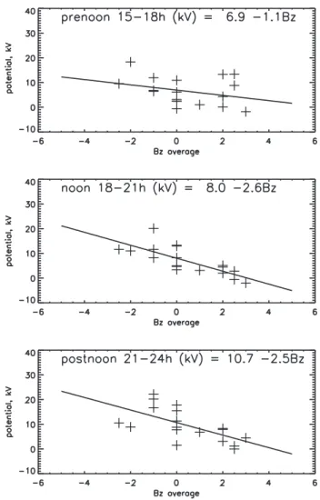
Figure 4 shows the integrated potential for 3×3 h intervals:
prenoon, noon, and postnoon as functions of IMF Bz. The
noon interval is the cusp interval as mentioned above. The potentials in all three intervals respond in a similar way to
Bz. The noon potential becomes negative (sunward convec-tion) for Bzabout +3 nT. This value agrees well with the Bz value when we begin to observe sunward convection in the polar cap (Jayachandran and MacDougall, 2001). It can also be seen that the potential in the prenoon interval is smaller than in either of the other two intervals. This shows the well known weakness of the dawn “convection cell” relative to the dusk convection cell (in the corotating coordinate sys-tem: see Newell et al. (2004, Paragraph 20). The noon and
16
Figure 4. Potentials calculated for three time intervals as a function of IMF Bz. The
equations of the fitted lines are shown.
Fig. 4. Potentials calculated for three time intervals as a function of
IMF Bz. The equations of the fitted lines are shown
postnoon intervals have about the same potentials.
It is of interest to compare these potentials with the cross polar cap potential that has been calculated in a number of studies (MacDougall and Jayachandran, 2001 and references therein). The estimated cross cap potential in that study, which used digital ionosonde measurements from polar cap
stations, was 8(kV)=44–10 Bz. This is very obviously a
much larger potential than is shown for the noon interval in Fig. 4. However, if one assumes that the cross cap potential is the sum of the 3 potentials shown in Fig. 4, then one obtains:
8(kV)=25.6–6.2 Bzfrom the integrated potentials, and this is comparable with the measured cross cap potentials. Some se-lective adjustment of the limits of the prenoon and postnoon intervals can give an even closer agreement, but even without such corrections it is obvious that the combined potentials of all three intervals are required to match the measured cross cap potential. Adding the 3 potentials shown on Fig. 4, and taking typical Bz as –3 nT, we find that only about 1/3 the polar cap potential is associated with convection through the noon cusp. This fractional result is similar to the numbers in a recent paper by Newell et al. (2004). We note that (see
1758 J. MacDougall and P. T. Jayachandran: Polar cap influx
17
Figure 5. Ratio of prenoon to postnoon potential as a function of IMF By.
Fig. 5. Ratio of prenoon to postnoon potential as a function of IMF
By.
values given on Fig. 4 plots) as the IMF Bz becomes more
negative the fraction of the total potential in the noon sector become larger.
This result is somewhat surprising in that the only obvious influx to the polar cap of open field line flux is through the noon cusp. However, the comparison of the potentials indi-cates that flux must have also entered the polar cap through the pre and post noon intervals. We will return to this prob-lem in the discussion.
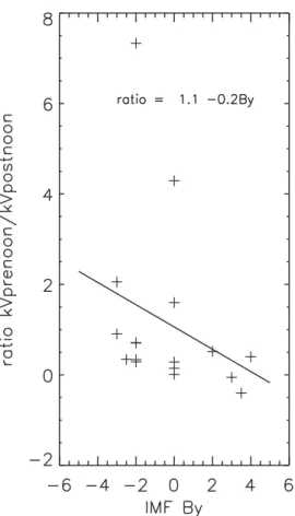
The remaining question in this section is whether there is an IMF By effect on the polar cap influx? Scatter plots of potentials as a function of Byshowed little obvious relation-ship, and yet the prevalence of By effects in the literature relating to the geometry of the influx to the polar cap made us look more closely to see if we could find a Byeffect.
In Fig. 5 the ratio of prenoon to postnoon potential is
shown as a function of IMF By. Although there is much
scatter in the data points, this figure shows the expected re-sult that the morning (prenoon) cell is stronger relative to the afternoon (postnoon) cell for more negative IMF By.
Comparison can be made here with the results of Newell et al. (2004) who found that their prenoon potential was larger than their postnoon potential for all IMF conditions. There is a difference in their definition of prenoon (time
<12:00 MLT) and postnoon (time >12:00 MLT) from what
we are using here (prenoon is time 07:00–10:00 MLT, post-noon is time 13:00–16:00 MLT). This difference in defining prenoon/postnoon only partly accounts for the difference be-tween the two sets of measurements. We attribute the remain-ing difference to the fact that IMF conditions for our data set are restricted to small values of IMF Bz and By in order to satisfy our data selection criteria.
3 Discussion
There appear to be several obvious solutions to the problem that the cusp convection only accounts for about 1/3 of the cross polar cap potential. Three of these are:
1. The cusp is actually much wider than 3 hours, at least intermittently.
2. The open region of the polar cap has a width compatible with the size of the cusp.
3. Most, ∼2/3, of the polar cap flux enters through the prenoon/postnoon cusp latitude regions.
We next discuss each of these three possibilities.
3.1 Is the cusp much wider than 3 hours?
The best way of locating the cusp is to use satellite parti-cle measurements. The study of cusp location by Apari-cio et al. (1991) using Viking satellite particle measurements shows it to be closely the 3 hour interval 10:00–13:00 MLT, although there is about a 1/2 h timeshift depending on the
sign of the IMF Bycomponent. Information about the cusp
width was also provided by Newell and Meng (1988), and Newell et al. (2004) using DMSP satellite data. In the Newell and Meng (1988) paper they presented statistics showing the probability of observing the cusp as a function of MLT. The curve is rather “Gaussian” so that it does not give an obvious width. However, if the cusp width is considered to be the full-width at half-maximum of the probability curve then the cusp width would be about 3 h. Therefore satellite particle data seems to support our usage of the 18:00–21:00 UT (10:00– 13:00 MLT) as the cusp interval, and certainly does not sup-port taking the whole 9-h interval from 07:00–16:00 MLT as the cusp interval. Further confirmation of the width used is from the studies of cusp width by Crooker et al. (1991), and Crooker and Toffoletto (1995). They found the maximum cusp width to be ∼3.5 h for high cross polar cap potential, so for the more moderate conditions in this study a 3-h width seems appropriate.
There are other ways of determining the cusp interval. Op-tical auroral observations initially detected the cusp gap as an interval at midday when auroral arcs disappeared and only red line auroral activity is seen. This was called the “midday auroral gap”. It was initially detected from ground optical observations, but can easily be seen in satellite images. Meng (1981) did a detailed study of the gap using both images and particle data from the DMSP satellites. Although he gives no
J. MacDougall and P. T. Jayachandran: Polar cap influx 1759
Table 1. Comparison of potentials from cusp and polar cap measurements.
Date (a) DMSP open cap width, km (b) Eureka antisunward speed, m/s (c)
Cross cap poten-tial from DMSP and Eureka, kV
(d)
Noon gap potential, kV
(e)
Total dayside po-tential, kV
30 Jan. 1996 1970 250 25 13.3 37.2
17 Feb. 1996 1970 300 30 13.0 24.3
19 Feb. 1996 1160 (457) 27 20.1 47.1
23 Jun. 1996 1200 300 18 5.0 15.9
statistical data about the width of the gap, he concludes that it is about 2–3 h wide. Based on our measurements and these other studies we conclude that the usual cusp width is only
∼3 h.
3.2 Is the width of open polar cap flux compatible with the cusp width?
One possibility is that the open flux in the polar cap only enters through the cusp and that the amount of open flux in the cap is compatible with this influx. There are many stud-ies of size and shape of the open polar cap. The study by Sotirelis et al. (1998) shows, in their Fig. 8, the measured amount of open polar flux versus the IMF Bz. For Bznear 0 nT, which pertains to most of our measurements shown in Fig. 4, they give the open flux as ∼400 MWb. Assuming, for simplicity, a circular open polar cap region and typical
B of ∼5.5×10⁻⁵T, their amount of open flux implies that
the diameter of the cap would be ∼3000 km. Since the 3-h cusp widt3-h is ∼1200 km t3-hen t3-he cusp flux could matc3-h to the polar cap flux if the polar cap antisunward convection speed was ∼1200/3000=0.4 of the cusp poleward speed. Es-sentially this implies that the flow through the cusp spreads out across the entire polar cap and therefore would flow an-tisunward at a much reduced speed relative to the speed in the cusp. We had convection measurements from our polar cap stations Eureka and Resolute Bay for most of the days that we selected. Typically, the average polar cap antisun-ward convection speeds were somewhat larger than the cusp speeds rather than smaller. Therefore the polar cap dimen-sions from published measurements do not support that the dimension of the open polar cap region is sufficiently small to match to the open flux entering through the cusp. As a fur-ther examination of whefur-ther the small cusp potential could be compatible with the cross cap potential on open field lines we examined DMSP particle measurements for several of our samples. The open, polar rain region of the polar cap can be quite easily identified on most satellite passes. Using a number of satellite passes throughout the day we estimated the polar cap dawn-dusk widths and these are shown in col-umn (a) of Table 1. The Eureka, and/or Resolute Bay average measured antisunward convection speeds for hours around 19:00 UT are given in column (b). For one case there was
no measured speed so we used an estimated speed calculated from the formula in Table 2 of MacDougall and
Jayachan-dran (2001) using the IMF Bz value (speed value shown in
braces). Combining the speed and width we calculated the cross cap potentials shown in column (c). These potentials can then be compared with our measured noon gap poten-tials shown in column (d), and the sum of the prenoon, noon, and postnoon potentials shown in column (e). It should be noted that to determine the dayside potentials in column (e) we had to integrate measured velocities over ∼9 h. These are therefore not an instantaneous measurement, although only days with relatively steady IMF were used.
The table shows that the noon gap potentials (d) alone are notably smaller than the cross cap potentials (c), whereas the total dayside potentials (e) are of comparable magnitude. This again shows that the second possible explanation of the inconsistency in the amount of convecting open polar cap flux and the flux through the noon cusp gap using the postu-lation of a narrow polar cap does not agree with observations. 3.3 Does most of the polar cap flux enter the polar cap in
the prenoon/postnoon intervals?
This seems to be the most likely scenario. Studying the DMSP particle data there is often a relatively sharp change from auroral activity to polar rain as the satellites pass into the polar cap in the prenoon/postnoon sectors. There is no obvious particle signature at the prenoon/postnoon polar cap boundary that is similar to the cusp signature seen at midday. Thus it seems that the flux that is passing into the polar cap in these sectors becomes open (reconnected) without showing a characteristic cusp particle signature.
Newell et al. (2004) show maps of DMSP satellite particle mapping to various magnetospheric regions. For these same prenoon/postnoon sectors they show Low Latitude Boundary Layer (LLBL) at about cusp latitudes. Then more poleward in these sectors they show Mantle (which extends across the entire dayside and is just the low energy ion “tail” precipita-tion seen on the open polar cap field lines), and finally polar rain in the central polar cap. The Mantle region is obviously open, but they are ambivalent as to whether the LLBL region is open or closed. This is obviously the region where we are seeing the E-region precipitation shown in Figs. 1 and 2.
1760 J. MacDougall and P. T. Jayachandran: Polar cap influx 18
T
1T
1T
0T
0T
1T
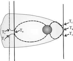
1Figure 6. Merging geometry for frontside and flank. Field lines (dashed) from the polar
cap are shown going (right) to the frontside merging point, and (left) to the flank merging point. The vertical lines are IMF –ve Bz. Merging time is T0 for both types of merging, and T1 mark the magnetic field kinks shortly after merging. The magnetopause is shown as a lightly shaded surface.
Fig. 6. Merging geometry for frontside and flank. Field lines (dashed) from the polar cap are shown going (right) to the frontside merging point, and (left) to the flank merging point. The vertical lines are IMF –ve Bz. Merging time is T0for both types of
merg-ing, and T1 mark the magnetic field kinks shortly after merging.
The magnetopause is shown as a lightly shaded surface.
There are a variety of transient auroral features in the prenoon and postnoon polar cap boundary regions. One type of transient feature observed in these regions are Poleward Moving Auroral Forms (PMAF). The properties of these PMAF were shown in studies by Shiokawa et al. (1996) and Sandholt et al. (2004). We can detect these PMAF in our CADI observations. The PMAF disappear after moving into the polar cap a few hundred kilometers, and can occasion-ally be detected by the CADI ionosonde at Resolute Bay
(86◦ mag. Lat.) but are never seen by the CADI further
poleward at Eureka. The study by Sandholt et al. (2004), looked carefully at the PMAF occurrence patterns and con-cluded that the PMAF were on reconnected open field lines. A second type of transient reconnection auroral feature is called a Pulsed Ionospheric Flow (PIF). Two studies of one of these are McWilliams et al., (2001a, b). The event that they studied started with transient reconnection just after the noon interval, and the reconnection region then moved rapidly tail-ward down the magnetopause flank. Associated with this PIF event are auroral and convection features near the afternoon polar cap boundary. Another similar event was described by Nishitani et al. (1999). A somewhat similar event studied by Milan et al. (2000) was not classified as a PIF but as a PMAF. There are therefore a variety of transient auroral features that are seen in the prenoon/postnoon intervals and are associ-ated with transient reconnection. A detailed review of the prenoon/postnoon polar cap boundary particle data and mag-netopause measurements by Cowley (1982) also showed that this region tends to be complex, and does not clearly show evidence for continuous reconnection.
The prenoon/postnoon sectors map to the flanks of the magnetosphere and there are several reasons why reconnection that is taking place on the flanks of the magne-tosphere (hereafter referred to as flank reconnection) could
have different characteristics from frontside reconnection. Firstly frontside reconnection may be steady or transient de-pending on the Alfv´enic conditions (Rodger et al., 2000). On the flanks of the magnetosphere the magnetosheath flow is supersonic and therefore the reconnection conditions are al-most always super Alfv´enic. Thus flank reconnection should likely be transient. The less steady convection velocities that we observe at Cambridge Bay directed into the polar cap at times before and after the cusp interval may be a signature of this transient reconnection.
A second difference arises from the shape of just-reconnected field lines on the flanks as compared to those on the frontside. While the frontside just-reconnected field lines are strongly kinked the just-reconnected flank lines will have much less of a kink. A sketch showing the kink ge-ometry is shown in Fig. 6. This sketch show frontside and flank merging, both marked as time T0, and the kinks in the reconnected field lines shortly after merging at time T1. As can be seen the field line geometry for flank merging is less kinked than for frontside merging. This means that there will be less energization of the plasma on the newly connected flank field lines. A third difference is that flank reconnection is to a supersonic downtail flowing magnetosheath plasma so that most reconnected particles will have considerable mo-mentum to overcome in order to precipitate in the earthward direction. This was discussed in Newell et al. (2004, see their Paragraph 15).
It therefore seems that flank reconnection has different characteristics from frontside reconnection. It is not clear whether there is a distinct dividing line between the two types of reconnection at any given time, or whether frontside re-connection can transition to flank rere-connection.
4 Conclusions
From digital ionosonde measurements we can often iden-tify the cusp region extending over 3 h from ∼10:00– 13:00 MLT. The convection into the polar cap is usually not high speed and the amount of open flux convecting through the cusp accounts for only about 1/3 of the polar cap flux. The majority of flux enters the cap through the ∼3 h wide prenoon/postnoon sectors on either side of the cusp. We attribute the relatively different characteristics of these prenoon/postnoon sectors, as compared to the cusp, to tran-sient flank merging that has somewhat different characteris-tics as compared to frontside steady merging.
Acknowledgements. This research was supported by grants from
the Canadian Natural Science and Engineering Research Coun-cil. WIND data was obtained from the Coordinated Data Analysis (CDA) Web. The authors thank P. T. Newell, JHU-APL, for making available DMSP particle data. The Cambridge Bay CADI was op-erated by technical personnel from NavCanada. The authors thank the referees for useful comments and suggestions.
Topical Editor M. Lester thanks K. Hosokawa and another referee for their help in evaluating this paper.
J. MacDougall and P. T. Jayachandran: Polar cap influx 1761 References
Aparicio, B., Thelin, B., and Lundin, R.: The polar cusp from a particle point of view: A statistical study based on Viking data, J. Geophys. Res., 14 023–14 031, 1991.
Austin, J. B., Murphree, J. S., and Woch, J.: Polar arcs: New results from Viking polar images, J. Geophys. Res., 98, 13 545–13 555, 1993.
Baker, K. B., Dudeney, J. R., Greenwald, R. A., Pinnock, M., Newell, P. T., Rodger, A. S., Martin, N., and Meng, C.-I.: HF radar signatures of the cusp and low-latitude boundary layer, J. Geophys. Res., 100(A5), 7671–7695, 1995.
Cowley, S. W. H., The causes of convection in the earth’s magne-tosphere: A review of developments during IMS, Rev. Geophys. Space. Phys., 20, 531–565, 1982.
Crooker, N. U., Toffoletto, F. R., and Gussenhoven, M. S.: Opening the cusp, J. Geophys. Res., 96, 3497–3503, 1991.
Crooker, N. U. and Toffoletto, F. R.: Global aspects of magnetopause-ionosphere coupling: Review and synthesis, in: Physics of the Magnetopause, Geophys. Monogr. Ser., vol. 90, edited by: Song, P., Sonnerup, B. U. O., and Thomsen, M. F., AGU, Washington, D.C., 363–370, 1995.
Grant, I. F., MacDougall, J. W., Ruohoniemi, J. M., Bristow, W. A., Sofko, G. J., Koehler, J. A., Danskin, D., and Andre, D.: Com-parison of plasma flow velocities determined by the ionosonde Doppler drift technique, SuperDARN radars, and patch motion, Radio Sci., 30, 1537–1549, 1995.
Gussenhoven, M. S., Hardy, A., Heinemann, N., and Burkhardt, R. K.: Morphology of the polar rain, J. Geophys. Res., 89, 9785– 9800, 1984.
Hones Jr., E. W., Craven, J. D., Frank, L. A., Evans, D. S., and Newell, P. T.: The horse-collar aurora: A frequent pattern of the aurora in quiet times, Geophys. Res. Lett., 16, 37–40, 1989. Jayachandran, P. T. and MacDougall, J. W.: Sunward polar cap
con-vection: J. Geophys. Res., 106(A12), 29 009–29 025, 2001. Lassen, K., Danielsen, C., and Meng, C.-I.: Quiet-time average
au-roral configuration, Planet. Space Sci., 36, 791–799, 1988. MacDougall, J. W. and Jayachandran, P. T.: Polar cap convection
relationships with solar wind, Radio Sci., 36, 1869–1880, 2001. McWilliams, K. A., Yeoman, T. K., and Cowley, S. W. H.:
Two-dimensional electric field measurements in the ionospheric foot-print of a flux transfer event, Ann. Geophys., 18, 1584–1598, 2001a,
SRef-ID: 1432-0576/ag/2000-18-1584.
McWilliams, K. A., Yeoman, T. K., Sigwarth, J. B., Frank, L. A., and Brittnacher, M.: The dayside ultraviolet aurora and convec-tion responses to a southward turning of the interplanetary mag-netic field, Ann. Geophys., 19, 707–721, 2001b,
SRef-ID: 1432-0576/ag/2001-19-707.
Milan, S. E., Lester, M., Cowley, S. W. H., and Brittnacher, M.: Convection and auroral response to a southward turning of the IMF: Polar UVI, CUTLASS, and IMAGE signature of transient magnetic flux transfer at the magnetopause, J. Geophys. Res., 105(A7), 15 741–15 755, 2000.
Newell, P. T. and Meng, C.-I.: The cusp and the cleft/boundary layer: Low-altitude identification and statistical local time varia-tion, J. Geophys. Res., 93, 14 549–14 556, 1988.
Newell, P. T. and Meng, C.-I.: Mapping the dayside ionosphere to the magnetosphere according to particle precipitation character-istics, Geophys. Res. Lett., 19, 609–612, 1992.
Newell, P. T., Xu, D., Meng, C.-I., and Kivelson, M. G.: Dynamical polar cap: A unifying approach, J. Geophys. Res., 102, 127–139, 1997.
Newell, P. T., Ruohoniemi, J. M., and Meng, C.-I.: Maps of precip-itation by source region, binned by IMF with inertial convection streamlines, J. Geophys. Res., 109, doi:10.1029/2004JA010499, 2004.
Nishitani, N., Ogawa, T., Pinnock, M., Freeman, M. P., Dudeney, J. R., Villain, J.-P., Baker, K. B., Sato, N., Yamagishi, H., and Mat-sumoto, H.: A very large scale flow burst observed by the Su-perDARN radars, J. Geophys. Res., 104 (A10), 22 469–22 486, 1999.
Rodger, A., Coleman, I. J., and Pinnock, M.: Some comments on transient and steady-state reconnection at the dayside magne-topause, Geopys. Res. Lett., 27, 1359–1362, 2000.
Sandholt, P. E., Farrugia, C. J., and Denig, W. F.: Dayside au-rora and the role of IMF |By|/|Bz|: detailed morphology and
re-sponse to magnetopause reconnection, Ann. Geophys., 22, 613– 628, 2004,
SRef-ID: 1432-0576/ag/2004-22-613.
Siscoe, G. L. and Huang, T. S.: Polar cap inflation and deflation, J. Geophys. Res., 90, 543–547, 1985.
Shiokawa, K., Yumoto, K., Nishitani, N., Hayashi, K., Oguti, T., McEwen, D. J., Kiyama, Y., Rich, F. J., and Mukai, T.: Quasi-periodic poleward motions of sun-aligned auroral arcs in the high-latitude morning sector: A case study, J. Geophys. Res., 101, 19 789–19 800, 1996.
Sotirelis, T., Newell, P. T., and Meng, C.-I.: Shape of the open-closed boundary of the polar cap as determined from observa-tions of precipitating particles by up to four DMSP satellites, J. Geophys. Res., 103, 399–406, 1998.
Wing, S., Newell, P. T., and Ruohoniemi, J. M.: Double cusp: Model prediction and observational verification, J. Geophys. Res., 106, 25 571–25 593, 2001.