Dynamic stability, blowoff, and flame characteristics of oxy-fuel combustion

Dynamic Stability, Blowoff, and Flame

Characteristics of Oxy-Fuel Combustion

by

Andrew Philip Shroll

B.S., Mechanical Engineering

University of Nebraska-Lincoln (2008)

Submitted to the Department of Mechanical Engineering

in partial fulfillment of the requirements for the degree of

Master of Science in Mechanical Engineering

at the

MASSACHUSETTS INSTITUTE OF TECHNOLOGY

June 2011

c

Massachusetts Institute of Technology 2011. All rights reserved.

Author . . . .

Department of Mechanical Engineering

May 6, 2011

Certified by . . . .

Ahmed F. Ghoniem

Ronald C. Crane (’72) Professor

Thesis Supervisor

Accepted by . . . .

David Hardt, Professor of Mechanical Engineering

Chairman, Department Committee on Graduate Theses

Dynamic Stability, Blowoff, and Flame Characteristics of

Oxy-Fuel Combustion

by

Andrew Philip Shroll

Submitted to the Department of Mechanical Engineering on May 6, 2011, in partial fulfillment of the

requirements for the degree of

Master of Science in Mechanical Engineering

Abstract

Oxy-fuel combustion is a promising technology to implement carbon capture and sequestration for energy conversion to electricity in power plants that burn fossil fuels. In oxy-fuel combustion, air separation is used to burn fuel in oxygen to easily obtain a pure stream of carbon dioxide from the products of combustion. A diluent, typically carbon dioxide, is recycled from the exhaust to mitigate temperature. This substitution of carbon dioxide with the nitrogen in air alters the thermodynamics, transport properties, and relative importance of chemical pathways of the reacting mixture, impacting the flame temperature and stability of the combustion process.

In this thesis, methane oxy-combustion flames are studied for relevance to natural gas. First, a numerical 1-D strained flame shows significantly reduced consumption speeds for oxy-combustion compared to air combustion at the same adiabatic flame temperature. Competition for the H radical from the presence of carbon dioxide causes high CO emissions. Elevated strain rates also cause incomplete combustion in oxy-combustion, demonstrated by the effect of Lewis number with a value greater than one for flame temperatures under 1900 K.

Most of this work focuses on experimental results from premixed flames in a 50 kW axi-symmetric swirl-stabilized combustor. Combustion instabilities, upon which much effort is expended to avoid in gas turbines with low pollutant emissions, are described as a baseline for the given combustor geometry using overall sound pressure level maps and chemiluminescence images of 1/4, 3/4, and 5/4 wave mode limit cycles. These oxy-combustion results are compared to conventional air combustion, and the collapse of mode transitions with temperature for a given Reynolds number is found. Hysteresis effects in mode transition are important and similar for air and oxy-combustion.

Blowoff trends are also analyzed. While oxy-combustion flames blow off at a higher temperature for a given Reynolds number due to weaker flames, there is an unexpected negative slope in blowoff velocity vs temperature for both air and oxy-combustion. The blowoff data are shown to collapse due to blowoff velocity being inversely proportional to the molar heat capacities of the burned gas mixtures at a

given power. Finally, particle image velocimetry results are discussed to relate flow structures to corresponding flame structures.

Thesis Supervisor: Ahmed F. Ghoniem Title: Ronald C. Crane (’72) Professor

Acknowledgments

I would like to thank Professor Ghoniem first and foremost for his guidance and insight on this project. His expertise and breadth of knowledge have inspired me in energy and combustion research. I also could not have made it without the help, direction, and many lessons from Santosh Shanbhogue. He has been critical to my progress as a student and researcher. The flame code and experimental setup of this thesis build off of previous work by Ray Speth, and I am grateful for his patience in imparting a sliver of his expertise to me. I owe much to the rest of the Reacting Gas Dynamics Lab as well for answering my many questions. It has been a pleasure working with everyone.

The help and support of my classmates and friends have been indispensable in my time at MIT. I am truly thankful for the friends I have from all the places I have lived. To my many teachers and mentors from MIT and UNL, as well as those outside academia, I thank them for their generosity and for developing a drive in me to make a difference. Most of all, I appreciate the love and support of my family. They have been with me every step of the way.

This work has been sponsored by King Abdullah University of Science and Tech-nology (KAUST), Grant number KSU-I1-010-01.

Contents

Abstract 4

Acknowledgments 5

1 Introduction 13

1.1 Oxy-Fuel Combustion for Carbon Capture . . . 13

1.2 Oxy-Fuel Combustion Dynamics . . . 15

1.3 Thesis Goals . . . 18

2 Experimental Setup 21 2.1 Equipment . . . 21

2.2 MATLAB Code . . . 24

2.3 Operating Conditions . . . 25

3 Numerical 1-D Strained Flame 27 3.1 Numerical Setup . . . 27

3.2 Flame Consumption Speed . . . 29

3.3 Temperature and Species Profiles . . . 34

3.4 Emissions Considerations . . . 35

3.5 Lewis Number Effect . . . 38

4 Combustion Dynamics 43 4.1 Oxy-Combustion Baseline Characteristics . . . 43

4.3 Frequency Ratio . . . 51 4.4 Hysteresis in Mode Transition . . . 54 4.5 Dynamics Conclusions . . . 59

5 Blowoff 61

5.1 Flame Modes and Blowoff . . . 62 5.2 Flow Fields from PIV . . . 67 5.3 PIV Challenges . . . 68

6 Summary and Future Work 79

6.1 Summary . . . 79 6.2 Suggested Future Work . . . 80

List of Figures

1-1 Temperature Reference Graph . . . 18

2-1 Combustor Model . . . 22

2-2 Swirler Model . . . 23

2-3 Swirler and Premixing . . . 23

2-4 Exhaust Configurations . . . 24

2-5 Operating Conditions . . . 26

3-1 Twin Flame Configuration . . . 28

3-2 Consumption Speed . . . 29

3-3 Consumption Speed at Selected Strain Rates . . . 30

3-4 Consumption Speed with Preheating . . . 31

3-5 Laminar Burning Velocity . . . 32

3-6 Laminar Burning Velocity at 1800 K for varied φ . . . 33

3-7 Flame Area Based on Laminar Burning Velocity . . . 33

3-8 Temperature Profiles at a = 10 and 250 s−1 for Tad = 2000 K . . . 34

3-9 Species Profiles at a = 10 and 250 s−1 for Tad = 2000 K . . . 36

3-10 Temperature Profiles at a = 250s−1 . . . 37

3-11 CO Profiles at a = 250s−1 . . . 37

3-12 Radical Species Profiles at a = 250s−1 . . . 40

3-13 O2 and CO output at 1800 K for varied φ . . . 41

3-14 CO Summary . . . 41

4-1 Dynamic response for oxy-combustion at Re = 20,000 . . . 44

4-2 Oxy Flame Images at Tad = 2200 K . . . 45

4-3 Oxy Flame Images at Tad = 2000 K . . . 46

4-4 Oxy Flame Images at Tad = 1900 K . . . 47

4-5 Dynamic response for air combustion at Re = 20,000 . . . 48

4-6 Air Flame Images at Tad = 2000 K . . . 49

4-7 Air Flame Images at Tad = 1900 K . . . 50

4-8 Comparison for Re = 15,000 to 30,000 . . . 52

4-9 Frequency maps for air and oxy-combustion. . . 53

4-10 Combustor frequencies . . . 54

4-11 Predicted frequencies . . . 55

4-12 Predicted frequency ratios . . . 55

4-13 Hysteresis shown by comparing increasing and decreasing sweeps . . . 56

4-14 Hysteresis based on ignition condition . . . 58

5-1 Oxy Flame Images at Re = 32,500 . . . 63

5-2 Flame Mode Maps for Open Exhaust . . . 64

5-3 Blowoff Velocity Comparison . . . 66

5-4 Blowoff Data Collapse . . . 66

5-5 Processed PIV Data at Tad = 2060 K . . . 68

5-6 Velocity Profiles at Tad = 2060 K . . . 70

5-7 Processed PIV Data at Tad = 1960 K . . . 71

5-8 Instantaneous PIV Data at 1960 K . . . 72

5-9 Processed PIV Data at Tad = 1890 K . . . 73

5-10 Velocity Profiles at Tad = 1890 K . . . 74

5-11 Processed Oxy-Combustion PIV Data at Decreasing Tad . . . 75

5-12 Processed Air Combustion PIV Data at Decreasing Tad . . . 76

5-13 Instantaneous PIV Data at 1790 K . . . 77

List of Tables

1.1 Mixture reference conditions at Tad . . . 19

1.2 Nomenclature . . . 20 4.1 Ratio of experimental frequencies (oxy/air) for each wave mode. . . . 54

Chapter 1

Introduction

Energy in valuable forms is an essential part of modern life. World-wide energy consumption continues to rise as a result of growing population and increased de-velopment in many countries. Currently, 85% of this energy is obtained from fossil resources, and there is an appreciable risk of anthropogenic climate change by contin-ued release of carbon dioxide into the atmosphere through combustion of these fuels [10]. One strategy to reduce the net amount of CO2 released is to sequester (pump

into the earth) the CO2 produced at power plants that convert the chemical energy in

fossil fuels into electricity. Oxy-fuel combustion, on which this thesis focuses, is one of the viable methods to capture carbon dioxide for sequestration. Carbon capture and sequestration (CCS) to prevent and/or alleviate anthropogenic climate change is thus the motivation for this work. More specifically, this thesis focuses on oxy-fuel combustion as applied to the field of combustion dynamics.

1.1

Oxy-Fuel Combustion for Carbon Capture

There are currently three major avenues toward CCS. The first is post-combustion capture, in which CO2 is separated from flue gasses in a traditional power plant.

This is generally accomplished with monoethanolamine absorption cycles. The second avenue is pre-combustion capture, where a scheme such as an integrated gasification combined cycle (IGCC) is used to produce synthesis gases which are burned in a way

that facilitates CCS. While pre-combustion capture could be used with natural gas via fuel reforming, the most promising route for pre-combustion capture is coal with IGCC because of the advantages IGCC provides in cleaning up a dirty fuel like coal. There are also other advanced capture schemes such as chemical looping currently being researched.

The third major avenue for CCS, oxy-fuel combustion (also written as oxy- bustion), is in itself not a new technology. The traditional meaning of oxy-fuel com-bustion is to burn a fuel in pure oxygen rather than in air, which contains only 21% oxygen by volume. Burning in pure oxygen allows for much higher flame tempera-tures because the inert nitrogen in air is no longer present as a heat sink. Common uses under this meaning include oxy-acetylene welding and heating of glass furnaces. Oxy-fuel combustion as applied to CCS, however, requires lower flame temper-atures to stay within the material limits in power plants. This implies that some diluent besides nitrogen must be used. The principle of oxy-combustion for CCS is burning fuel in a mixture of oxygen and a diluent that is recycled from the flue gas. Since the products of combustion are carbon dioxide and water, one of these two is used. The products (flue gas) are then comprised (ideally) of only CO2 and H2O. The

water is then condensed, providing a pure stream of CO2 for sequestration. Carbon

dioxide is currently being studied the most as the diluent of choice, but Richards et al. [28] have put significant effort into H2O dilution.

Oxy-combustion is generally associated with coal because it is a more likely target for CCS: a coal power plant produces about three times as much CO2 per unit of

electric energy as a natural gas combined cycle (NGCC) power plant. However, natural gas power plants should also be considered for oxy-combustion because, for example, about 19% of electricity generation in the U.S. is from natural gas [8]. In addition, the substantial increase in natural gas reserves from shale gas technology in recent years suggests there will be significant growth, especially in North America, in the amount of electricity produced from natural gas.

Each of the types of carbon capture includes an energy penalty, and in oxy-fuel combustion the main penalty is in separating the oxygen out of air. Energy is also

needed to pump CO2 into the ground for sequestration or an application such as

en-hanced oil recovery (EOR). The most common industrial scale air separation method is cryogenic distillation. Kvamsdal et al. [18] showed that the efficiency penalty of CCS for NGCC with cryogenic separation is about on par with post-combustion cap-ture. Oxy-combustion shows a clear advantage in efficiency, however, when coupled with an advanced separation method such as an ion transport membrane (ITM).

While excellent retrofit potential is claimed for oxy-combustion of natural gas in boiler systems [32], there are challenges in retrofitting existing gas turbines for oxy-combustion. Although existing compressors and turbines could be used, a gas turbine designed for the new working fluid (mostly CO2) would be required to avoid a drop

in performance [6, 15].

1.2

Oxy-Fuel Combustion Dynamics

The premixed mode of combustion is susceptible to instabilities, which are a feedback process between combustion, heat release, and the acoustic field. There have been a number of reviews on this topic [22, 14] that detail various mechanisms leading to instability and control strategies. However, there is a need for further studies to understand several remaining questions regarding, for example, mode transitions (how the flow/combustion characteristics couple with a particular mode or its harmonics during any change in operating conditions such as loading, reactants, temperature and fuel characteristics).

In general, the transition in the stability characteristics of the combustor, from stable to unstable or from one mode to its harmonics, can be lumped into two cat-egories. The first kind of transition occurs when the flame-stabilization mechanism changes for a small change in conditions, such as from a wake mode to a shear layer mode and vice-versa [16, 11]. The second kind of transition involves the same mecha-nism, but the transition is due to the non-linearity associated with the physics of the problem. Some explanations for this behavior include non-normality [26], hysteresis [23] or the nature of the flame-acoustic describing-function [27].

Most of the above studies deal with a single fuel, and the conditions used to ini-tiate the transition involve changing either the equivalence ratio or flow speed. Some work also looks at the effect of fuel structure and inlet reactant temperature. For oxy-combustion, fuel and air are expected to be in stoichiometric or near stoichio-metric proportions, so it remains to be seen whether there is a fundamental property that can predict mode transitions. For natural gas-air mixtures, Fritsche and co-workers [9] proposed a Damkohler number that non-dimensionalizes the effect of flow velocity on mode transitions. Work with synthesis-gas fuel blends showed that the transitions occur for critical values of a non-dimensional strained flame consumption speed [30, 12]. It was shown that, for a given equivalence ratio and flow velocity, changing the CO:H2 ratio of the fuel impacts the stability characteristics and mode

transition, although the variation in adiabatic flame temperature (Tad) is small. For

a given equivalence ratio, changing the fuel composition from 80:20 H2:CO to 20:80

changes Tad by roughly 100K and drastically alters the stability of the combustor.

However, such a change in stability cannot be reproduced if Tad is increased for a

fixed fuel composition by raising the equivalence ratio. It appears then that the key parameter that predicts the mode switch is another combustion property such as the consumption speed. The prediction of mode-switching based on a strained flame con-sumption speed works well for hydrogen enriched mixtures, where the flame speed incorporates the fundamental characteristics of hydrogen such as high diffusivity and unique kinetics.

Little work has been done on oxy-fuel combustion issues in gas turbines until re-cently [17, 21]. However, a number of groups have begun presenting experimental data. Ditaranto et al. [7] presented acoustic mode results from a 2 kW premixed, expansion-stabilized combustor. Williams et al. [33] used a premixed, 20 kW swirl-stabilized combustor to show that CO emissions do not become significant until an equivalence ratio greater than 0.95 for oxy-combustion, and at this point CO emissions rise more quickly for oxy-combustion than air. Amato et al. [2, 3] used a combustor built the same as Williams’ and showed that high equivalence ratio and tempera-ture are associated with excessive CO. They also discussed ways diluents can impact

the flame, such as mixture specific heat (which affects flame temperature), transport properties (thermal conductivity, mass diffusivity,viscosity), chemical kinetic rates (both CO2 and H2O are both chemically active), and radiation. Kutne et al. [17]

used a 30 kW partially premixed swirl-stabilized combustor at atmospheric pressure, experiencing thermo-acoustic instabilities over a substantial range of operating condi-tions. They stated a higher sensitivity in performance to oxygen concentration than equivalence ratio. Other bench scale tests have been conducted, such as Glarborg et al. [13] with a 0.1 kW isothermal reactor. They discussed chemistry, stating that CO2 competes with O2 for H via CO2+H⇔CO+OH, while CO2+O⇔CO+O2 and

CO2+OH⇔CO+HO2 are relatively slow. Liu et al. [24] also showed numerically

that the overall reaction rate of CH4/O2/CO2 mixtures is much slower compared to

CH4/O2/N2 mixtures primarily because of the competition for the H radical. The

demonstration of these effects on flame speed date to Law et al. [36], who showed experimentally that methane flames burning in oxygen-CO2 mixtures have laminar

burning velocities approximately one eighth of those burning in air when the oxygen mole fraction is kept at 21%.

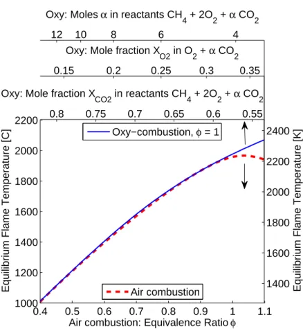
A useful reference for comparing oxy-combustion and air combustion is the adi-abatic flame temperature. Although there is an extra degree of freedom in mix-ture composition by controlling the amount of diluent in oxy-combustion, near-stoichiometric conditions are desired to avoid any excess oxygen in the combustion products. Therefore in Figure 1-1 air combustion temperature is plotted versus equiv-alence ratio, and stoichiometric oxy-combustion temperature is plotted versus a re-versed and shifted axis of diluent CO2 mole fraction in the CH4/O2/CO2 mixture

or O2 mole fraction in the O2/CO2 mixture to make comparisons convenient. To

be clear, the reactant mixtures are φCH4 + 2(O2 + 3.76 N2) for air and CH4 +

2O2 + αCO2 for oxy-combustion, where φ and α are varied. The adiabatic flame

temperature given is the calculated equilibrium temperature for the reactant inlet temperature at 300 K. In this document, the mole fraction of CO2 is defined as the

mole fraction in the reactant mixture, not the mole fraction in O2 plus CO2. The

0.4 0.5 0.6 0.7 0.8 0.9 1 1.1 1000 1200 1400 1600 1800 2000 2200

Air combustion: Equivalence Ratio φ Equilibrium Flame Temperature [C] _{Air combustion}

0.55 0.6 0.65 0.7 0.75 0.8 1400 1600 1800 2000 2200 2400 Oxy: Mole fraction X

CO2 in reactants CH4 + 2O2 + α CO2

Equilibrium Flame Temperature [K]

Oxy−combustion, φ = 1

0.15 0.2 0.25 0.3 0.35

Oxy: Mole fraction X

O2 in O2 + α CO2

12 10 8 6 4

Oxy: Moles α in reactants CH

4 + 2O2 + α CO2

Figure 1-1: Adiabatic (equilibrium) flame temperature comparison for air and oxy-combustion.

the mole fraction of O2 in O2 plus CO2 is also shown.

Because Tad is used often throughout this document, it will be helpful to reference

Table 1.1 for reactant conditions at 100 K intervals. The value for α is the number of moles added to the reactants CH4 + 2O2. Since φOXY is unity in this case, XCO2

is simply _3+αα .

1.3

Thesis Goals

Successful implementation of oxy-combustion technology requires addressing two chal-lenges concerning the aerothermodynamic design of the combustor. First, the sub-stitution of nitrogen with carbon dioxide as a diluent alters the thermodynamics,

Table 1.1: Mixture reference conditions at Tad

AIR OXY, φ=1 OXY, φ=1

Tad [K] φ α XCO2 1600 0.562 9.28 0.756 1700 0.617 8.27 0.734 1800 0.674 7.38 0.711 1900 0.734 6.56 0.686 2000 0.798 5.80 0.659 2100 0.868 5.08 0.629 2200 0.956 4.38 0.593

transport properties and relative importance of chemical pathways of the reacting mixture, impacting the flame temperature and stability of the combustion process. Second, as in air combustion, the flue gas stream must contain minimal emissions and trace gases, particularly carbon monoxide, nitric oxide and, in the case of oxy-combustion, oxygen. However, the goal of this work is not to design gas turbines; rather, the aim is to characterize oxy-combustion at a fundamental level.

Chapter 2 describes the experimental setup, instrumentation and diagnostics. In Chapter 3, a one-dimensional strained flame code is used to gain insight into turbulent combustion of methane in air and oxy-combustion environments and illustrate the dif-ferences between CH4/air and CH4/O2/CO2 flames. Chapter 4 presents experimental

data on dynamic mode transitions for oxy-fuel combustors. The broader objective of this effort is to explore the dynamic stability characteristics of oxy-combustion and to compare the characteristics of oxy-combustion and air combustion in order to develop predictive tools for combustor design and retrofit. Results are compared to CH4/air mixtures for a range of Reynolds numbers. This chapter is closed with

a brief overview of the non-linear behavior of the stability characteristics. Chapter 5 presents results for an open-exhaust configuration which removes thermoacoustic instabilities and facilitates the study of fundamental characteristics such as flame structure, flow structure, and blowoff. Finally, Chapter 6 summarizes this work and provides recommendations for future research.

Table 1.2: Nomenclature Tu Unburned (reactant) temperature

Tad Adiabatic flame temperature

φ Equivalence ratio α Moles of CO2

XCO2 Mole fraction CO2 in reactants (including fuel)

a Strain rate

SL Laminar burning velocity

Sc Flame consumption speed

Chapter 2

Experimental Setup

2.1

Equipment

The combustor, shown in Figure 2-1, is designed to stabilize combustion using a combination of swirl and sudden expansion. Premixed CH4/O2/CO2 or premixed

CH4/air enters the combustor through a 38 mm diameter inlet pipe. The swirler is

located 5 cm upstream of the expansion plane and has 8 blades with an estimated swirl number of 0.53 [19]. The swirler can also be moved flush with the dump plane, which has an effect on the dynamics, but this was found to cause excessive heating of the swirler. From the expansion plane downstream, the inner diameter is 76 mm. The first 40 cm downstream where the flame is anchored consists of a quartz tube for optical access. The overall acoustic length of the combustor (from the choke plate to the end of exhaust tube) is 4.5 m. The flow is choked upstream to prevent equivalence ratio oscillations and provide a known acoustic boundary condition (u0 = 0).

Air, CO2, O2, and CH4 are each supplied using Sierra Instruments mass flow

controllers capable of supporting a thermal power of 50 kW. The accuracy of each is +/- 1% of full scale with a repeatability of +/- 0.2% of full scale, but special note should be made here of issues with the flow accuracy. Another piece of Sierra equipment, a 780s flow meter, was used to find a proportional offset for the air flow controller such that (actual flow rate) = 0.96∗(apparent flow rate). During oxy-combustion, CO2 flows through the same controller; however, the correction factor

Mass flow controllers Exhaust Quartz tube Swirler Pressure sensors Choke plate Fuel bar Oxygen inlet CO₂inlet Expansion plane 440 cm 55 cm 31 cm 90 cm

Figure 2-1: Model of axisymmetric swirl combustor.

is not used for the CO2 flow rate because additional calibration equipment would be

required. An additional zero offset correction of 3.9 standard liters per minute of CH4 is used for the fuel mass flow controller. The flow rate of O2 in the third controller,

used only in oxy-combustion, is assumed to be within the specified accuracy.

Two Kulite MIC-093 pressure transducers are used to record pressure oscillations 11 cm and 52 cm downstream of the choke plate at 10 kHz.

For the chemiluminescence images presented in Sections 4.1 and 4.2, high speed images are recorded at 500 fps using a MEMRECAM GX-1 high speed camera fitted with a 50mm f/1.8 lens. A 2mm thick CG-BG-39 Schott-glass is placed in front of the camera to block out infrared radiation. The field of view in all the images starts at the dump plane of the combustor and extends about 22.8 cm downstream. Images are post-processed by normalizing the intensities in each image with the maximum intensity of the brightest image in an instability cycle.

A model of the swirler is shown in Figure 2-2. While premixed combustion is the focus of this work, an injection tube was installed through the centerbody of the swirler in order to try non-premixed combustion, as shown in Figure 2-3. This resulted, however, in long flames with bright, even sooty tips. The reason for this undesirable flame behavior is likely due to excessive jet penetration of the fuel through the inner recirculation zone due to high fuel to oxidizer velocity ratios, affecting the flow structure and mixing significantly. Therefore, only premixed combustion is presented for the given geometry. Even with the tubing through the centerbody, the

Figure 2-2: Model view of swirler. The inside diameter of the flow area is 1.5 inches. A fuel injection tube is inserted through the centerbody for non-premixed combustion capability.

Figure 2-3: Cutaway view of swirler and expansion plane zone showing plumbing for premixed and non-premixed combustion.

centerbody acts as a small bluff body because there is no flow through the tube for premixed combustion.

Another hardware switch that can be toggled is the exhaust configuration. Shown in Figure 2-4 (a), the closed exhaust configuration is used to study combustion dy-namics (Chapter 4) with the previously described acoustic length of 4.5 m. The second configuration, shown in (b), consists of an open exhaust annulus at the end of the quartz tube. With the acoustic length significantly shortened, phenomena such as blowoff can be studied without combustion dynamics (Chapter 5). The blue arrows indicate room air that is drawn into the exhaust at room pressure.

(a) Closed exhaust (b) Open exhaust

Figure 2-4: (a) Closed exhaust configuration for studying combustion dynamics and (b) open exhaust configuration to remove instabilities.

2.2

MATLAB Code

A custom Matlab code is used for control, data acquisition, and processing. The con-trol portion includes a graphical user interface which communicates with the mass flow controllers via COMM ports. Digital outputs (fuel shutoff solenoid valve, camera and PIV triggering) and analog inputs (thermocouples, pressure transducers, photomul-tiplier tube) are fed through an NI BNC-2110 connector block and an NI PCIe-6259 data acquisition card. The interface allows a flow parameter to be chosen to hold constant during tests. For all runs presented in this work, Reynolds number is held constant and temperature is varied by changing φ in air combustion and XCO2 in

oxy-combustion. Mean inlet velocity, total mass flow rate, and power output are all dependent variables. During operation, live plots of all flow rates and an FFT of the pressure signal are displayed to monitor dynamic modes. Data can be logged in multiple sessions without restarting the combustor.

In each test which sweeps across temperature, the set conditions (flow rates) are held constant for a few seconds before switching φ or XCO2 to the next set

tempera-ture. The processing code then looks for periods of time in which the flow conditions are constant within a specified tolerance and produces an output for each. These outputs are binned and reduced to plots such as the ones shown in Figure 4-8.

2.3

Operating Conditions

Shown in Figure 2-5 are the approximate operating ranges for the combustor in air and oxy-combustion modes. The purpose of this plot is to display the conditions of operation because a basis of comparison must be established for the two modes. The flame is generally ignited and brought near 2200 K. Next, the temperature (and power) are gradually reduced along the line of constant Re for the Reynolds number at which the combustor is ignited. The lower temperature limit determined by blowoff, generally between 1600 K and 1700 K.

For a given Reynolds number and adiabatic flame temperature, the power output of oxy-combustion is lower. For example, at Re = 20,000 and Tad = 1800 K, the fuel

flow rate for oxy-combustion is 0.37 g/s, while the fuel flow rate is 0.44 g/s for air. Likewise, the total mass flow rate and mean inlet velocity are lower for oxy-combustion at 9.4 g/s and 5.2 m/s versus 10.8 g/s and 8.0 m/s for air. In air combustion, the mean inlet velocity change is small when the equivalence ratio is changed to adjust the temperature at constant Reynolds number. However, the mean inlet velocity changes more significantly in oxy-combustion at constant Reynolds number when changing the temperature because the bulk properties change with XCO2. One should also

consider which parameters are varied with varying load (turn-down ratio) in gas turbine operation.

0 10 20 30 40 50 60 70 2 4 6 8 10 12 14 16 ←Re 15k Re 15k→ ←Re 20k Re 20k→ ←Re 25k Re 25k→ ←Re 30k Re 30k→ ←Re 35k Re 35k→ Power [kW]

mean inlet velocity [m/s]

Oxy Air 1600 K 1900 K 2200 K constant Re

Figure 2-5: Constant temperature contours at three arbitrary temperatures for the combustor in air and oxy-combustion as a function of thermal power output for dif-ferent Reynolds numbers at Tu = 300 K. In oxy-combustion, φ = 1 and CO2 dilution

is varied. In air combustion, φ < 1. Note that blowoff actually occurs before 1600 K is reached in constant Reynolds number tests (see Chapter 5). This plot applies to both exhaust configurations shown in Figure 2-4.

Chapter 3

Numerical 1-D Strained Flame

As discussed in Chapter 1, the laminar burning velocity of CH4/O2/CO2 mixtures are

one eighth of CH4/air mixtures for an oxygen mole fraction of 21%. For these mixtures

the oxy-combustion flame temperature is much lower due largely to the roughly 65% larger heat capacity of CO2 on a molar basis. The interest, however, is in comparing

flames at the same flame temperature, and the difference in burning velocity is still significant. Given that flames in turbulent flows are subjected to strains, the interest is in computing the strained flame consumption speed. This provides the mixture fractions of CO2 for which the strain rates anticipated in experiments exceed the

extinction strain rates for oxy-fuel mixtures.

3.1

Numerical Setup

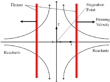
A one-dimensional strained flame code is used to compute the consumption speed for varying strain rates. The laminar flame is stabilized in a planar stagnation flow and shown in Figure 3-1, where the opposed twin flame configuration allows extinction to occur at higher strain rates when the flames are pushed closer together. The resultant potential flow velocity field is characterized by the strain rate parameter a. The stretch rate κ of the planar flame under steady conditions is simply κ = a.

Governing equations for the flame structure are found by using a boundary layer approximation across the flame thickness. CHEMKIN and TRANSPORT libraries

Figure 3-1: Twin Flame configuration for 1-D strained flame simulation. This config-uration allows extinction to occur when the strain rate is high enough that the flame front is pushed close to the stagnation point.

are used to evaluate chemical source terms and the various physical properties. A modified version of the GRI-Mech 3.0 kinetic model is used where the nitrogen-containing species have been removed except for N2 in the air cases. Radiation effects

are not considered in the model. Further details of the model can be found in Speth et al. [31]. The consumption speed Sc of the flame is defined as

Sc =

R∞

−∞q000/cpdx

ρu(Tb− Tu)

where q is the volumetric heat release rate, cp is the specific heat of the mixture,

x is the coordinate normal to the flame, ρu is the unburned mixture density, and Tu

and Tb are the unburned and burned temperature, respectively. Extrapolating the

consumption speed to a strain rate of zero gives the laminar burning velocity.

All cases are at atmospheric pressure, and the reactant temperature is 300 K in all cases except as described in Figure 3-4. The proper mixture compositions for the given adiabatic flame temperatures are calculated using CANTERA with GRI-Mech 3.0 by equilibrating the mixture at constant enthalpy and pressure (complete combustion is not assumed).

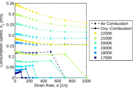
0 200 400 600 800 1000 0 0.05 0.1 0.15 0.2 0.25 0.3 0.35 Strain Rate, a [1/s] Consumption Speed, S c [m/s] _{Air Combustion} Oxy−Combustion 2200K 2100K 2000K 1900K 1800K 1700K

Figure 3-2: Consumption speed vs strain rate a for Tads from 1700 K to 2200 K,

where Tu = 300 K. The oxy-combustion equivalence ratio is φ = 1.

3.2

Flame Consumption Speed

The consumption speed at a given strain rate for a mixture is one of the major outputs of interest, and the differences between air and oxy-combustion are significant. Shown in Figure 3-2 are consumption speeds for air and oxy-combustion at equal adiabatic flame temperatures from 1700 K to 2200 K. Here again φ in air combustion and α in oxy-combustion are varied to change Tad. At 2200 K the consumption speed of the

oxy-combustion flame is roughly half that of air. At lower temperatures the difference is more extreme, where oxy-combustion consumption speed is less than 5 cm/s, or one fourth that of air. Clearly the substitution of N2 with CO2 in the oxy-combustion

flames adversely affects the chemical and/or transport time scales.

Also important in characterizing flame behavior is the condition at which extinc-tion occurs. Instances of extincextinc-tion (five for oxy, one for air) are shown in Figure 3-2 where the consumption speed drops to zero. Since strain rates on the order of 250 s−1 are expected in the experiments for similar conditions [30], sustainable oxy-combustion flames are not expected to exist at or below 1800 K. As will be shown though, experimental flames exist at temperatures well below this value. One possible

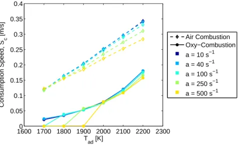
1600 1700 1800 1900 2000 2100 2200 23000 0.05 0.1 0.15 0.2 0.25 0.3 0.35 0.4 T ad [K] Consumption Speed, S c [m/s] Air Combustion Oxy−Combustion a = 10 s−1 a = 40 s−1 a = 100 s−1 a = 250 s−1 a = 500 s−1

Figure 3-3: Consumption speed vs Tad, where Tu = 300 K. The oxy-combustion

equivalence ratio is φ = 1.

reason is the turbulent effects of local mixing on pockets of products and reactants. Taking the information from Figure 3-2 and plotting Sc against temperature for

se-lected strain rates in Figure 3-3, one can see the near linear dependence of Sc on

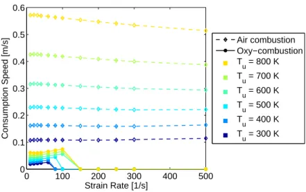
temperature for air combustion and a non-linear dependence for oxy-combustion. Since one might ideally wish to compare premixed oxy-combustion to lean pre-mixed air combustion, consumption speed comparisons are also made for an adiabatic flame temperature of 1400◦C. In these cases, the reactant temperature is varied from 300 K to 800 K, and the equivalence ratio in air combustion and the CO2 mole

frac-tion in oxy-combusfrac-tion are still varied to maintain an adiabatic flame temperature of 1400◦C. This temperature is suitable for gas turbines which operate under load at an equivalence ratio near 0.6 to achieve low NOx emissions and to stay within the

material limitations of the turbine. Therefore, results from the 1-D strained flame code at 1400◦C are shown in Figure 3-4, and the difference between air and oxy-combustion is drastic. Even when the oxy-oxy-combustion mixture is preheated to 800 K, the consumption speed is still well below that of air for a reactant temperature of 300 K.

0 100 200 300 400 500 0 0.1 0.2 0.3 0.4 0.5 0.6 Strain Rate [1/s] Consumption Speed [m/s] Air combustion Oxy−combustion T u = 800 K T u = 700 K T_u = 600 K T_u = 500 K T_u = 400 K T_u = 300 K

Figure 3-4: Consumption speed vs strain rate a for Tad=1400◦C, where Tu ranges

from 300 to 800 K. The oxy-combustion equivalence ratio is φ = 1.

obtain the laminar burning velocity (SL). The laminar burning velocity has been

shown to be significantly lower for methane oxy-combustion, both for varied equiva-lence ratio at 21% O2 in the oxidizer and for stoichiometric CO2 dilution compared

to stoichiometric N2 diluted mixtures for varied dilution amounts (see Chen et al.

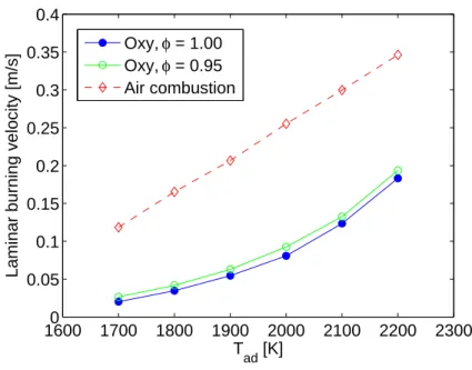
[5]). What is novel, however, is to plot laminar burning velocity as a function of adiabatic flame temperature as shown in Figure 3-5. Interestingly, SL appears linear

for air combustion, while SL increases more quickly at higher temperatures for

oxy-combustion. These values of SL match well with values from a similar CHEMKIN

model.

In addition to plotting stoichiometric oxy-combustion in Figure 3-5, oxy-combustion for an equivalence ratio of 0.95 is also plotted at the same temperatures. This means that at φ = 0.95, slightly fewer moles of CO2 are required to obtain products at the

same temperature in the reactants φCH4 + 2O2 + αCO2. The laminar burning

ve-locity is a small amount higher for φ = 0.95, presumably because the adverse effects of CO2 on chemical time scales is lower. This upward trend in SL for decreasing

equivalence ratio at constant (fixed) Tad for oxy-combustion can be continued, and

is shown in Figure 3-6. The curve represents a vertical slice from Figure 3-5 at Tad

16000 1700 1800 1900 2000 2100 2200 2300 0.05 0.1 0.15 0.2 0.25 0.3 0.35 0.4 T ad [K]

Laminar burning velocity [m/s]

Oxy, φ = 1.00 Oxy, φ = 0.95 Air combustion

Figure 3-5: Laminar burning velocity vs adiabatic flame temperature for Tu = 300 K.

to φ = 0.148 on the left. At this minimum equivalence ratio for combustion at 1800 K, there is no carbon dioxide, and the reactants are only methane (0.148 moles) and oxygen (2 moles).

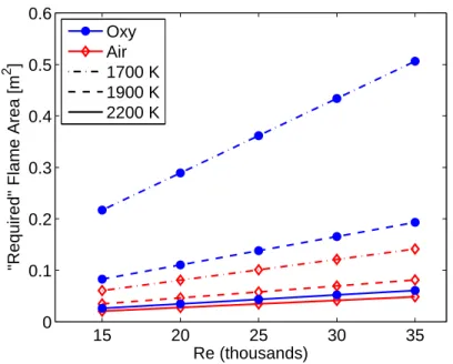
Because of the low flame speeds in oxy-combustion, proportionally larger flame areas should be required for wrinkled laminar flames, and long, weak flames are expected. However, shown in Figure 3-7 is the effective required area for a wrinkled flame, comparing air and oxy-combustion at the same Reynolds numbers for three temperatures. This flame area is given by A = _ρm˙

uSL, where ˙m, ρu, and SL are the

total mass flow rate, unburned gas density, and laminar burning velocity for the mixture, respectively. At 2200 K, the area needed for oxy-combustion is only 25% higher than air. Furthermore, images in Chapter 4 from high speed video show a remarkable similarity with air combustion in not only flame structure but also flame size. At lower temperatures, though, the theoretical area is several times larger for oxy-combustion.

0 0.2 0.4 0.6 0.8 1 0 0.05 0.1 0.15 0.2 ←No CO 2 7.35 moles CO 2→ T ad = 1800 K

Oxy−combustion equivalence ratio, φ S L

[m/s]

0 1 2 3 4 5 6 7

Moles of CO

2 in reactants

Figure 3-6: Laminar burning velocity vs oxy-combustion equivalence ratio for Tu =

300 K. To keep Tad constant at 1800 K, the amount of CO2 dilution is varied from

zero at φ=0.148 to the highest amount at φ=1.0.

15 20 25 30 35 0 0.1 0.2 0.3 0.4 0.5 0.6 Re (thousands)

"Required" Flame Area [m

2 ] Oxy Air 1700 K 1900 K 2200 K

Figure 3-7: Flame area based on SL, where Tu = 300 K. The oxy-combustion

0 20 40 60 80 0 500 1000 1500 2000 distance x [mm] Temperature [K] Oxy−combustion Air combustion a = 10 s−1 a = 250 s−1

Figure 3-8: Temperature profiles at a = 10 and 250 s−1 for Tad = 2000 K, where Tu

= 300 K. The oxy-combustion equivalence ratio is φ = 1.

3.3

Temperature and Species Profiles

Basic outputs of the strained flame code that provide insight into flame characteristics include temperature and species profiles. Shown in Figure 3-8 are temperature profiles for air and oxy-combustion for two strain rates at a set Tad = 2000 K. Following the

flow from right to left, toward the stagnation point at x = 0, reactants enter at 300 K. Next, in the reaction zone, the temperature rises steeply to the burned gas temperature. The distance of the flame from from the stagnation point is the steady-state distance for the flame at a given strain rate. For both strain rates, the CH4/air

flame resides at a greater distance from the stagnation point because of the higher consumption speed. At a = 250s−1, the flames are ”pushed” closer to x = 0. To see the temperature profiles more clearly at a = 250s−1, refer to Figure 3-10.

Shown in Figure 3-9 are species profiles of O2, CH4, CO, and CO2 for two strain

rates which correspond to the temperature profiles in Figure 3-8. In oxy-combustion, the amount of incoming fuel is half the amount of oxygen due to the stoichiometric mixture, while the amount of fuel in air combustion is less than half the amount of

oxygen because φ = 0.8. One can also get a feel for the amount of CO2 that would

need to be recycled from the products in reality to obtain the desired inlet conditions, for this case about 87%. At the higher strain rate of 250 s−1, the effect of stretch becomes apparent in oxy-combustion from the significant amount of oxygen left over and excessive CO remaining by the time the mixture reaches the stagnation point. Also note the difference in x-axis scales in Figure 3-9 (a) and (b).

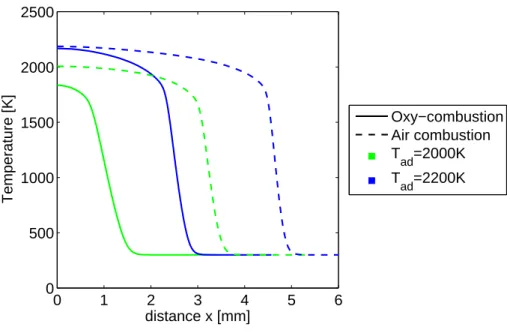
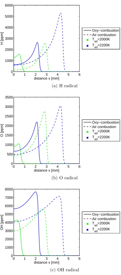
Next, an example case is explored for profiles at a single strain rate of 250 s−1 and two temperatures in order to demonstrate the importance of temperature. The prod-ucts of air and oxy-combustion shown, in Figure 3-10, each reach their set temperature at 2200 K, but oxy-combustion at 2000 K falls short by 165 K. This is evidence of a weak flame with partial extinction, and the impact on CO levels is shown in Figure 3-11. Each of the CO ”outputs” at the stagnation plane overshoots the equilibrium value. For instance, oxy-combustion CO at 2200 K overshoots by 50%, but at 2000 K the overshoot is 400% due to the incomplete combustion. To glean some information on the chemical impact of CO2 without a detailed chemical analysis, consider Figure

3-12. Noting the air and oxy-combustion curves at Tad = 2200 K, where both reach

the set Tad, the relative peak heights of H and OH can be viewed as a demonstration

of competition for the H radical in CO2+H⇔CO+OH. More H is consumed via the

reaction in oxy-combustion due to the presence of CO2, resulting in lower ppm values

of H and higher values of OH as well as CO.

3.4

Emissions Considerations

Rather than NOx and CO as the emissions of interest in air combustion, the most

important emissions in oxy-fuel combustion of natural gas are CO and O2. There is

a trade-off between emitting these two species, as shown in Figure 3-13 for varied φ in oxy-combustion while holding Tad at 1800 K and a low strain rate of a = 10s−1.

The values of CO and O2 shown are the levels in the products when they reach

the stagnation point. The crossover point at about φ = 0.97 is similar to that seen experimentally at φ = 0.95 by Li et al. [21]. Williams et al. [33] also experimentally

0 20 40 60 80 0 0.1 0.2 0.3 0.4 0.5 0.6 0.7 0.8 distance x [mm] Mole Fraction Oxy−combustion Air combustion O 2 CH 4 CO CO 2 (a) a = 10s−1 0 1 2 3 4 5 6 0 0.1 0.2 0.3 0.4 0.5 0.6 0.7 distance x [mm] Mole Fraction Oxy−combustion Air combustion O 2 CH 4 CO CO 2 (b) a = 250s−1

Figure 3-9: Species Profiles of O2, CH4, CO, and CO2 at (a) a = 10s−1and (b)

a = 250s−1 for air and oxy-combuation at Tad = 2000 K. Tu = 300 K and the

0 1 2 3 4 5 6 0 500 1000 1500 2000 2500 distance x [mm] Temperature [K] Oxy−combustion Air combustion T ad=2000K T ad=2200K

Figure 3-10: Temperature profiles at a = 250s−1 for Tads of 2000 K and 2200 K,

where Tu = 300 K. The oxy-combustion equivalence ratio is φ = 1.

0 1 2 3 4 5 6 0 2 4 6 8 x 104 distance x [mm] CO [ppm] Oxy−combustion Air combustion T ad=2000K T ad=2200K Oxy Equilibrium Air Equilibrium

Figure 3-11: CO profiles at a = 250s−1 for Tads of 2000 K and 2200 K, where Tu =

300 K. The oxy-combustion equivalence ratio is φ = 1. Point values correspond to equilibrium CO at Tad.

showed surprisingly low CO values until φ > 0.95 for CH4/O2/CO2 flames at a fixed

O2 concentration.

Especially at lower temperatures, the equilibrium values of CO for stoichiometric oxy-combustion are orders of magnitude higher than for air combustion. This is the starting point for Figure 3-14, shown with continuous lines. Next, values of CO at the stagnation point are plotted for varied strain rates for set adiabatic flame temperatures from 1700 K to 2200 K. In air combustion, CO values at a = 10s−1 nearly match equilibrium, and CO increases much more quickly with strain rate at lower temperatures (kinetic effects). Values for oxy-combustion behave similarly, only with a much higher starting point. It is also interesting to note that for mixtures such that Tad ≤ 1900 K, CO levels at even the lowest strain rates do not approach

equilibrium. Rather, at Tad = 1700 K and a = 10s−1, CO exceeds 1.5 %. The

x-axis values for these points changes with strain because the temperature used is the maximum temperature for that strain rate. Therefore, Lewis number effects (which may also lead to partial extinction effects) are expected to be the cause of this shift in burned gas temperature. Overall, the impact of residence time on CO emissions is important, and the distance at which the flame resides from the stagnation point affects the levels shown.

3.5

Lewis Number Effect

For a positively stretched flame such as the stagnation flame used in this chapter, Law [20] showed that the mixture Lewis number has important effects on properties such as temperature and extinction strain. It is known that Le < 1 for methane-air mixtures, and in Figure 3-15, the curves for air combustion at multiple adiabatic flame temperatures are consistent with the curve in [20] for Le < 1. The tempera-ture increases slightly with increasing strain until near extinction, where the curve changes concavity and the value decreases. For Le > 1, the temperature monotoni-cally decreases with increasing strain. This effect is clearly exhibited at Tad= 1700 K,

however, where there is less CO2 in the mixture, it appears that the Lewis number

0 1 2 3 4 5 6 0 1000 2000 3000 4000 5000 6000 distance x [mm] H [ppm] Oxy−combustion Air combustion T ad=2000K T ad=2200K (a) H radical 0 1 2 3 4 5 6 0 500 1000 1500 2000 2500 3000 3500 distance x [mm] O [ppm] Oxy−combustion Air combustion T_ad=2000K T ad=2200K (b) O radical 0 1 2 3 4 5 6 0 1000 2000 3000 4000 5000 6000 7000 8000 distance x [mm] OH [ppm] Oxy−combustion Air combustion T_ad=2000K T ad=2200K (c) OH radical

Figure 3-12: H, O and OH radical profiles at a = 250s−1 for Tads of 2000 K and 2200

0.9 0.92 0.94 0.96 0.98 1 0 0.005 0.01 0.015 0.02 0.025 0.03

Oxy−combustion equivalence ratio, φ

Mole Fraction T ad = 1800 K O 2 CO

Figure 3-13: O2 and CO output at constant Tad = 1800 K for Tu = 300 K. The strain

rate is a = 10s−1. 1600 1800 2000 2200 100 101 102 103 104 ← a10 ← a10 ← a250 ← a10 ← a10 ← a10 ← a10 ← a250 ← a10 ← a10 ← a250 ← a10 ← a10 ← a250 ← a250 ← a10 ← a10 ← a250 ← a250

T_ad for Equilibrium; T_burned for strained [K]

CO [ppm] Air Combustion Oxy−Combustion T_ad=1700K T_ad=1800K T_ad=1900K T_ad=2000K T ad=2100K T ad=2200K Equilibrium CO

Figure 3-14: CO output vs Temperature for Tu = 300 K. Continuous lines are

equi-librium values, and points are strained flame values for set values of Tad from 1700

K to 2200 K and strain rates a = [10 30 60 100 150 200 250]s−1. At a given mix-ture setting (set Tad), the CO output increases with increasing strain, and the actual

flame temperature shifts according to Lewis number effects with increasing strain. The oxy-combustion equivalence ratio is φ = 1.

101 102 1500 1600 1700 1800 1900 2000 2100 2200 2300 Strain rate [s−1] Maximum temperature [K] Oxy Air T_ad = 1700 K T_ad = 1800 K T ad = 1900 K T ad = 2000 K T ad = 2100 K T ad = 2200 K Set T ad

Figure 3-15: Lewis number effect. Maximum flame temperature vs strain rate a for set values of Tad from 1700 K to 2200 K, where Tu = 300 K. The oxy-combustion

Chapter 4

Combustion Dynamics

This chapter presents results for the combustor described in Chapter 2. In all cases, the Reynolds number is based on the 0.0381 m (1.5 inch) inlet diameter, the mean inlet velocity, and the reactant density and viscosity at 300 K. All oxy-combustion experiments are conducted at φ = 1.

4.1

Oxy-Combustion Baseline Characteristics

To understand the baseline stability characteristics of the combustor, consider Figure 4-1. This figure plots the Overall Sound Pressure Level (OASPL) as a function of CO2 mole fraction for stoichiometric CH4/O2 mixtures at Re = 20,000 for different

amounts of CO2 dilution. The OASPL measurements are taken using the transducer

placed just upstream of the expansion plane. In this figure as well other OASPL plots throughout the paper, the symbols have been colored based on the frequency of the instability.

For low dilution levels (Tad = 2230 K), the flame is very compact and the sound

pressure levels exceed 160 dB. The dominant instability frequency is 132 Hz, which corresponds to the five-quarter wave mode of the combustor. High speed flame im-ages for this mode show that the flow oscillates between a double-helix type vortex breakdown (as seen visually by experimental observation of flame filaments) and a configuration in which it flashes back (see Figure 4-2).

As the dilution levels are increased, the combustor remains unstable at roughly the same amplitude, though the contribution of the five-quarter wave mode to the OASPL decreases and the three-quarter wave mode (83 Hz) increases.

At XCO2 = 0.63 (Tad = 2100 K) the combustor abruptly transitions to the

three-quarter wave mode while maintaining the same limit-cycle amplitude. High speed images for this condition indicate that the flow-structures are now different, with the flow structures switching between a double-helix type and a spiral type breakdown during the instability cycle (see Figure 4-3). The type of structures observed are surmised visually during experiments.

As the dilution levels are increased from XCO2 = 0.63 (Tad = 2100 K) to XCO2 =

0.67 (Tad = 1970 K), the apparent flame length increases, commensurate with what is

expected when decreasing the flame temperature. The flame dynamics are controlled by the fluid mechanics of the inner recirculation zone as was reported in work on propane-air mixtures [19]. 0.58 0.6 0.62 0.64 0.66 0.68 0.7 0.72 0.74 130 135 140 145 150 155 160 165 170 175 OASPL [dB] Mole Fraction X CO2 Peak Frequency [Hz] 0 50 100 150 200 1700 1800 1900 2000 2100 2200 T ad [K]

(a) OASPL for Re = 20,000

Frequency [Hz] X CO2 0.6 0.62 0.64 0.66 0.68 0.7 0.72 0 50 100 150 200

Sound Pressure Level, dB

110 120 130 140 150 160

(b) Frequency spectrum for Re = 20,000

Figure 4-1: OASPL (a) and spectrum (b) of oscillations as a function of adiabatic flame temperature for CH4/O2/CO2 mixtures at Re = 20,000. For reference, note

the two x-axes in (a).

The next abrupt transition is seen at XCO2 = 0.67 (Tad = 1970 K) where the

instability jumps from the three-quarter wave mode to the quarter wave mode with a slightly lower limit-cycle amplitude. For this case though, there is a step jump in flame length (Figure 4-4). This mode persists until XCO2 = 0.7 (Tad = 1850 K) when the

Figure 4-2: Sequence of images in a cycle during the five-quarter wave mode for CH4/O2/CO2 flames with XCO2 = 0.594 (Tad = 2200 K) at Re = 20,000. Images are

2ms apart.

flame switches to a columnar type, similar to the ones reported by Zhang et al. [35] and Muruganandam et al. [25]. No instability is observed in the frequency-spectra for these cases.

So far the results have been plotted as a function of XCO2, corresponding to

adi-abatic flame temperatures in the 1700-2200 K range. Now, consider the flame speeds for these mixtures: If the dilution is adjusted to get Tad = 2050K in a CH4/O2/CO2

mixture (conditions matching Figure 4-3), the computed laminar burning velocity is 10 cm/s. For CH4/air mixtures, this flame speed value is well below the flame speed

at the laminar flammability limit, namely 15 cm/s. It is surprising then that a rea-sonably compact flame is observed for these conditions. However, turbulent mixing likely plays a critical role in maintaining the compact flame in oxy-combustion.

Figure 4-3: Sequence of images in a cycle during the three-quarter wave mode for CH4/O2/CO2 flames with XCO2 = 0.659 (Tad = 2000 K) at Re = 20,000. Images are

2ms apart.

4.2

Comparisons with CH

/Air Flames

OASPL curves similar to the one plotted in Figure 4-1 are plotted in Figure 4-5 for CH4/air mixtures at the same Reynolds number, i.e. 20,000. The results indicate

that the dynamic response of the combustor is essentially similar to that presented in Section 4.1 for oxy-fueled mixtures in two ways. First, as the adiabatic flame temperature is decreased (in this case by turning down the equivalence ratio), the instability modes transition from the five-quarter wave mode to three-quarter to the quarter wave mode before eventually blowing off.

The second similarity is in the overall turbulent flame structure. For this consider Figure 4-6 and Figure 4-7. The adiabatic flame temperature and Reynolds number for these cases have been adjusted to match the conditions in Figure 4-3 and Figure 4-4, respectively. Looking at these figures side by side, the visible turbulent flame shapes are very similar as are the underlying vortex breakdown modes. These results suggest that the underlying flow-field is a strong function of the temperature jump

Figure 4-4: Sequence of images in a cycle during the quarter wave mode for CH4/O2/CO2 flames with XCO2 = 0.686 (Tad = 1900 K) at Re = 20,000. Images

across the flame. Some subtle differences exist for instance, in Figure 4-7 (CH4/air),

a waist is seen between the bubble upstream and the double-helix downstream. This structure is a bit weak in Figure 4-4a (CH4/O2/CO2). Since the mass flow rates

are nearly the same, differences in flame speed would lead the oxy-flame to bulge laterally to a larger volume to burn the same mass. Still, the mode transitions and flame geometries are clearly controlled by the flame temperature at a given Reynolds number, at least to the first order.

0.6 0.7 0.8 0.9 1 135 140 145 150 155 160 165 170 175 OASPL [dB] Equivalence Ratio φ 1700 1800 1900 2000 2100 2200 T_ad [K] Peak Frequency [Hz] 0 50 100 150 200

(a) OASPL for Re = 20,000

Frequency [Hz] φ 0.65 0.7 0.75 0.8 0.85 0.9 0 50 100 150 200

Sound Pressure Level, dB

110 120 130 140 150 160

(b) Frequency spectrum for Re = 20,000

Figure 4-5: OASPL (a) and spectrum (b) of oscillations as a function of adiabatic flame temperature for CH4/air mixtures at Re = 20,000. For reference, note the two

x-axes in (a).

OASPL comparisons between air combustion, in which the equivalence ratio is varied, and stoichiometric oxy-combustion, in which the CO2 mole fraction is varied,

for constant Reynolds numbers from 15,000 to 30,000 are shown in Figure 4-8. The equivalence ratio is maintained at unity in all the oxy-combustion tests. Each curve represents one test sequence in the combustor from ignition at the high temperature end toward blowout at the lower end. Because the mixtures are varied in different ways between the air and oxy-combustion cases, the adiabatic flame temperature for the given mixture is used as the abscissa. Small gradients in color from point to point show mild frequency shifts (as the burnt gas temperature decreases w.r.t the reactants; this is expected, see Speth [12]).

Figure 4-6: Sequence of images in a cycle during the three-quarter wave mode for CH4/air flames with φ = 0.798 (Tad = 2000 K) at Re = 20,000. Images are 2ms

apart.

While weaker flames are expected in oxy-combustion, because of the significant change in the consumption speed [36], surprisingly, similar dynamic modes and tran-sitions seen in air combustion and oxy-combustion. With the exception of Re = 30,000, mode transitions collapse well when using the adiabatic flame temperature across the two combustion modes. At Re = 25,000, for instance, there is one clear transition at Tad = 2100 K from the five-quarter mode to the three-quarter mode and

another at Tad = 1950 K from the three-quarter mode to the quarter-wave mode.

Strongest instabilities, those over 165 dB, exist at higher flame temperatures where a compact unstable flame exists in 3/4 or coexisting 3/4 and 5/4 wave modes. These peak frequencies are shown in Figure 4-9 that plot the frequency spectrum (truncated up to 250 Hz) as a function of the adiabatic flame temperature. The right and left edges of each plot are simply the condition at which data recording begins and the condition at blowout, respectively, so there is variation between plots. In oxy-combustion, the dominant frequencies for the high, medium, and low frequency modes are in the ranges of 125-150 Hz, 80-100 Hz, and 25-40 Hz, respectively. Frequencies

Figure 4-7: Sequence of images in a cycle during the quarter wave mode for CH4/air

for the three modes are shifted higher for air to 150-170 Hz, 100-120 Hz, and 30-50 Hz. The shift, as discussed in Section 4.3, is due to the differences in acoustic properties of the products and reactants between air and oxy-combustion. While the quarter wave mode exists alone in all cases, the three-quarter and five-quarter wave modes coexist in an overlap region. The five-quarter wave mode is dominant at the highest temperatures. The temperature range where modes coexist diminishes with increasing Reynolds number.

As the flame temperature is decreased by changing the mixture composition, tran-sitions occur to lower harmonics. In some cases, namely air combustion at all Reynolds numbers except for 15000, a hole exists (e.g. between Tad = 1930 K and 1980 K for

Re = 20,000) in this transition where the flame is considerably more stable. The sound pressure levels for these conditions are much lower for air flames compared to oxy-flames. The reason for this is not entirely clear, but is a subject of future investigation.

Regardless of whether the fuel is burned in air or in O2/CO2, the low frequency

(quarter-wave) unstable flames are several times longer than the compact unstable flame. A stable columnar flame that extends well into the exhaust is seen at the lowest temperatures for all Reynolds numbers before blowoff where the OASPL drops off significantly.

4.3

Frequency Ratio

The limit cycle frequencies corresponding to the previous figures are shown in Figure 4-10. The lowest frequencies correspond to the 1/4 wave mode, and the 3/4 wave mode is shown by the middle grouping. The 5/4 wave mode also exists as a dominant mode at high temperatures for all cases except oxy-combustion at Re = 30,000 and air combustion at Re = 15,000 (for these two cases, the 5/4 wave mode can be seen as co-existing in Figure 4-9). It is expected that if the combustor was completely adiabatic, the limit cycle frequency would be relatively insensitive to the Reynolds number. This expectation comes from compact flame acoustic models, where the

1600 1700 1800 1900 2000 2100 2200 2300 130 135 140 145 150 155 160 165 170 175 OASPL [dB] Air Combustion Oxy−Combustion (a) Re = 15,000 1600 1700 1800 1900 2000 2100 2200 2300 130 135 140 145 150 155 160 165 170 175 OASPL [dB] Air Combustion Oxy−Combustion (b) Re = 20,000 1600 1700 1800 1900 2000 2100 2200 2300 130 135 140 145 150 155 160 165 170 175 OASPL [dB] T_ad [K] Air Combustion Oxy−Combustion (c) Re = 25,000 1600 1700 1800 1900 2000 2100 2200 2300 130 135 140 145 150 155 160 165 170 175 OASPL [dB] T ad [K] Air Combustion Oxy−Combustion Peak Frequency [Hz] 0 50 100 150 200 (d) Re = 30,000

Figure 4-8: OASPL comparison as a function of adiabatic flame temperature for Re = 15,000 to 30,000.

length of the flame Lf is much less than the acoustic wavelength λ, i.e. Lf/λ  1.

For the cases shown, the worst case is approximately Lf/λ = 0.1. In actuality, the

frequency climbs with Re. Speculations for the cause include heat loss affecting the acoustic properties or the effect of Re on flow structure. If the flow structure is affected, a change in the coupling of heat release, flow, and acoustics could cause the frequency shift. The frequency for oxy-combustion is always lower, and the ratio for each mode and Reynolds number are summarized in Table 4.1. Using Equation (10) from Altay et al. [1], the expected resonant frequencies are plotted against Tad in

Figure 4-11. These curves match the experiments fairly well. Note, however, that the equation does not predict which mode will exist at each temperature, so the curves span the entire operating range. The predicted frequency ratios (fOXY/fAIR) are

Frequency [Hz] Re = 15000 16000 1700 1800 1900 2000 2100 2200 2300 50 100 150 200 Frequency [Hz] Re = 20000 16000 1700 1800 1900 2000 2100 2200 2300 50 100 150 200 Frequency [Hz] Re = 25000 16000 1700 1800 1900 2000 2100 2200 2300 50 100 150 200 Frequency [Hz] Re = 30000 T_ad [K] 16000 1700 1800 1900 2000 2100 2200 2300 50 100 150 200

Sound Pressure Level, dB 110 120 130 140 150 160 (a) Oxy-combustion Re = 15000 16000 1700 1800 1900 2000 2100 2200 2300 50 100 150 200 Re = 20000 16000 1700 1800 1900 2000 2100 2200 2300 50 100 150 200 Re = 25000 16000 1700 1800 1900 2000 2100 2200 2300 50 100 150 200 Re = 30000 T ad [K] 16000 1700 1800 1900 2000 2100 2200 2300 50 100 150 200

Sound Pressure Level, dB

110 120 130 140 150 160 170

(b) Air combustion

Figure 4-9: Frequency maps for air and oxy-combustion for Re = 15,000 to 30,000.

shown in Figure 4-12. These three ratio curves lie within the envelope created by the speed of sound ratio (cOXY/cAIR), where the speed of sound c =

√

γRT (assuming an ideal gas mixture) is dependent on the mixture specific heat ratio γ and the gas constant R. The upper bound is created by using only unburned mixture properties and the lower bound by using only burned mixture properties. Based on the average experimental ratio of 0.8 from Table 4.1, it can be concluded that, at least to first order, the change in dynamic frequency from air to oxy-combustion is explained by

1600 1700 1800 1900 2000 2100 2200 2300 20 40 60 80 100 120 140 160 180 200 T ad [K] Frequency [Hz] Air Oxy Re 15k Re 20k Re 25k Re 30k

Figure 4-10: Experimental frequencies. acoustic properties of the mixtures.

Table 4.1: Ratio of experimental frequencies (oxy/air) for each wave mode. Re 1/4 wave mode 3/4 wave mode 5/4 wave mode

15,000 0.86 0.76

20,000 0.75 0.77 0.82

25,000 0.88 0.79 0.83

30,000 0.78 0.80

4.4

Hysteresis in Mode Transition

For all the cases presented so far, the experiments were conducted by igniting the mixture at high equivalence ratios or high O2 fraction and then gradually lowering

it until blowoff. Results collected in this case indicate that there are two distinct transitions: a transition from the 3/4 to 1/4 wave mode at high temperatures, and another from the 1/4 wave mode to stable case at lower temperatures close to blowoff. Now, consider results from experiments conducted in the reverse order by increas-ing the equivalence ratio or O2 concentration (and hence the temperature) gradually

1600 1700 1800 1900 2000 2100 2200 20 40 60 80 100 120 140 160 180 T ad [K] Frequency [Hz] Air combustion Oxy combustion 1/4 Wave mode 3/4 Wave mode 5/4 Wave mode

Figure 4-11: Predicted frequencies as a function of adiabatic flame temperature for the three modes seen experimentally.

1600 1700 1800 1900 2000 2100 2200 0.81 0.815 0.82 0.825 0.83 0.835 0.84 T ad [K]

Frequency Ratio (Oxy/Air) 1/4 Wave mode_{3/4 Wave mode} 5/4 Wave mode

Figure 4-12: Predicted frequency ratios comparing air and oxy-combustion for the three modes seen experimentally.

until high temperatures are reached. These data are illustrated in Figure 4-13(a) for air and Figure 4-13(b) for oxy-fuel mixtures. This figure shows that the instability at the 1/4 wave mode persists for much higher flame temperatures before transitioning to the 3/4 wave mode, if the experiments are conducted by increasing the adiabatic flame temperature.

(a) Air combustion

(b) Oxy-combustion

Figure 4-13: Hysteresis shown by comparing increasing and decreasing sweeps at Re = 20k.

load-ing is increased or decreased, that is, it depends on the state and the history. At this point the interest is in determining whether the transitions depend on the tempera-ture pathway or are function of the pathway followed by some other state variable. For this purpose, another experiment was conducted; this time the combustor was ignited and immediately switched to Tad = 2030 K. According to Figure 4-5, at this

point the combustor should be in the 3/4 wave mode as per the decreasing tempera-ture path; but just at the border of the transition between the 1/4 to 3/4 wave mode as per the increasing temperature path. Once ignited the equivalence ratio was then gradually decreased. The trajectory of the limit cycle amplitude as a function of the temperature is illustrated in Figure 4-14. The figure shows that despite the decreasing temperature, the trajectory followed by the amplitude overlaps with the trajectory obtained as if the temperature was increased. This proves that the hysteresis in mode transitions is not just a function of temperature (and thus independent of the types of mixtures being burned). An area of future tests is to identify a state variable that controls the hysteresis, but so far the data suggests that this is dependent on the in-stability frequency the combustor is in just prior to the point when the temperature is increased or decreased.

One should also note that the trajectories (and consequently the blowoff limits) deviate below Tad = 1940 K. This is in turn due to the hysteresis of the 1/4 wave

mode with respect to the stable mode. Stated differently, if the combustor is ignited and suddenly brought to Tad = 1810K, the combustor is observed to be stable. The

temperature has to be increased to Tad = 1890K to kick it into the 1/4 wave mode.

However if the combustor is brought to Tad = 1890K slowly from higher temperatures

when the 1/4 wave mode is present, the same mode persists until lower temperatures. Considering the effects of the hysteresis, the data that was presented throughout this document was recorded by increasing the flame temperature after ignition until the combustor is kicked into the five-quarter mode, and then decreasing the tem-perature gradually. For CH4/Air mixtures, one could argue that this is guaranteed

by always starting at stoichiometric conditions and then decreasing the temperature. However, for CH4/O2/CO2mixtures, the maximum temperature that can be attained

Figure 4-14: Mode history dependence for air combustion at Re = 20,000. For the decreasing sweep, the test was conducted by igniting the flame at Tad = 2030 K and

then decreasing gradually.

is Tad = 3051K; but this was not possible given the temperature limitations of this

combustor. Hence the amount of dilution in the flow was reduced just enough to trigger the five-quarter wave mode.

Finally, for both air and oxy-combustion, the shift in transition temperature be-tween the 1/4 and 3/4 from hysteresis is on the order of 50 K. However, the quiet transition region between the 1/4 and 3/4 unstable modes is extended for air combus-tion and introduced for oxy-combuscombus-tion. That is, a significantly more stable flame can be achieved at 2000 K for oxy-combustion by approaching the corresponding mixture composition while in the low frequency mode. As a result, the space of oper-ation where the sound pressure level is over 165 dB is significantly decreased for the increasing sweeps. Making use of phenomena such as this could be exploited as an operation strategy for gas turbines.

4.5

Dynamics Conclusions

In this chapter the combustion dynamics characteristics of CH4/O2/CO2mixtures and

CH4/Air mixtures are compared in a swirl stabilized combustor. Although weaker

flames are expected in oxy-combustion due to lower consumption speed, the flame structures of air and O2/CO2 flames in each of the modes are similar. The transitions

from one instability mode to another are shown to be a function of the mixture adiabatic flame temperature for Re ≤ 25,000. The data match less well for Re = 30,000; the reasons for this could include heat transfer effects in the non-adiabatic combustor. Additional strained flame calculations with an asymmetric configuration having products on one side (unlike the twin flame configuration in Chapter 3) could potentially provide more relevant values for Scthat explain combustor behavior. The

data also reveal hysteresis with respect to mode transitions, which are shown to be mode-dependent and not temperature dependent. This fact could be exploited for developing control strategies to avoid a particular mode of instability. Another important note that increases the significance of flow structure and its complexity is that the range of Reynolds numbers from 15,000 to 35,000 used in this chapter and Chapter 5 are likely in the transition to turbulence range. That is, the flow is not yet fully developed because large scale structures in the vortex breakdown of the swirling flow are a function of Re. Therefore, the combustor behavior should be less dependent on Re above some critical Reynolds number.