Baffle material characterization for Advanced LIGO

Baffle Material Characterization for

Advanced LIGO

by

Cassandra R. Hunt

Submitted to the Department of Physics

in partial fulfillment of the requirements for the degree of

Bachelor of Science in Physics

at the

MASSACHUSETTS INSTITUTE

May 2008

OF TECHNOLOGY

@ Cassandra R. Hunt, MMVIII. All rights reserved.

The author hereby grants to MIT permission to reproduce and

distribute publicly paper and electronic copies of this thesis document

in whole or in part.

Author ... :...

v

DeptrLment

of Physics

May 9, 2008

Certified by ...

Nergis Mavalvala

Professor

Thesis Supervisor

Accepted by ...

David Pritchard

Chairman, Professor

ARCHVES

JUN 13 2008

LIBRARIES

Baffle Material Characterization for Advanced LIGO

by

Cassandra R. Hunt

Submitted to the Department of Physics on May 9, 2008, in partial fulfillment of the

requirements for the degree of Bachelor of Science in Physics

Abstract

The transition to Advanced LIGO introduces new sensitivity requirements for the LIGO interferometers. When light scatters away from the main laser beam, then scatters off the beam tube and returns to the main beam, noise is introduced into the phase of the laser. The Auxiliary Optics Support subsystem uses baffles and beam dumps to control this scatter, but the baffle material and shape contribute some scatter as well. Careful selection of baffle material for Advanced LIGO is necessary in order to minimize baffle backscatter. Characterization of potential materials will also inform the geometry and placement of baffles. To this end, I developed a scat-terometer experiment designed to measure the Bidirectional Reflectance Distribution Function (BRDF) of a material. The arrangement was used to measure the BRDF for black welder's glass, the prime candidate material for baffles in Advanced LIGO. I found that black glass has a BRDF on the order of 10- , putting it within sensitivity requirements.

Thesis Supervisor: Nergis Mavalvala Title: Professor

Acknowledgments

I owe a large debt of gratitude to Mike Zucker for supervising me on this project, for all his input, patience, and good humor. I would also like to thank Rich Mittleman for his role introducing me to LASTI and helping me find this project, as well as for good conversation about all things from LIGO to life. Thank you also to Nergis Mavalvala for agreeing to be my supervisor, and for all her help whipping this thesis into shape.

My mom and dad, Laura and William Hunt, shaped my inquisitiveness and drive with their encouragement, and I appreciate their efforts to instill in me the value of hard work and scholarship.

Contents

1 Introduction and Motivation 11

1.1 W hat is LIGO? ... 11

1.1.1 Seismic Isolation ... 12

1.2 Baffles in Advanced LIGO ... 13

2 Theory of Optical Scattering 15 2.1 Smooth vs. Rough Surfaces ... 15

2.2 The BRDF ... 16 2.3 Surface Scatterers ... 17 2.4 Bulk Scatterers ... 18 3 Previous Work 19 4 Scatterometry Apparatus 21 5 Measuring the BRDF 25 5.1 CCD Image Energy Level Calibration . ... 25

5.2 Approximating the Incident Beam . ... . 29

6 Near-Specular BRDF 35 6.1 R esults . . . .. . 35

6.2 Surface Contaminants ... 35

6.3 Error Sources and Result Robustness . ... 36 7

7 Large-Angle BRDF

7.1 Results ... ... 39

List of Figures

1-1 Diagram of LIGO Interferometer. . ... . 12

1-2 Light scatter in the interferometer arms. . ... 14

2-1 Pictorial representation of the BRDF. . ... 17

4-1 A diagram of the scatterometer. ... ... . .. 22

4-2 The rotating mount. ... 23

5-1 Intensity profile and beam spot on a Lambertian surface. . ... . 27

5-2 Beam profile using the razor blade method ... 29

5-3 CCD camera linearity. ... 32

5-4 Finding the beam waist using the razor blade method. . ... 33

5-5 Converting pixels to length. ... 33

6-1 Intensity profile and beam spot on black glass. . ... 36

6-2 Beam images and BRDF for three locations on black glass... . 37

6-3 Viewing surface contaminants. ... .. . . 38

6-4 The effect of varying the incident beam waist. . ... 38

7-1 BRDF for black glass over a range of incident beam angles. ... 40

Chapter 1

Introduction and Motivation

1.1

What is LIGO?

The Laser Interferometer Gravitational-Wave Observatory (LIGO) is a project de-signed to detect cosmic gravitational waves. Gravitational waves are the radiation of the gravitational force predicted by general relativity, a gravitational analog to light, the radiation of the electromagnetic force. Gravitational waves are emitted whenever masses accelerate, but because they are so weak, direct detection has not yet been achieved[14]. LIGO searches for cosmic sources of gravitational waves such as collisions of compact stars, inspirals, and oscillations of neutron stars and black holes.

Currently, LIGO can detect neutron star-neutron star (N-N) inspirals within a distance of 20 MPc[24]. LIGO is a multi-phase project, with plans to become more sensitive in stages. As of the writing of this paper, LIGO has just completed its final science run of the first stage, dubbed Initial LIGO. Construction has begun on Enhanced LIGO, an intermediate stage preceding construction of Advanced LIGO, which will be a major upgrade of the detector. For N-N inspirals, the range of Advanced LIGO is expected to increase by more than an order of magnitude[24].

1.1.1

Seismic Isolation

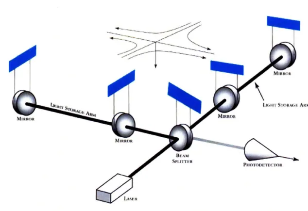
The optical configuration of the detector is a Michelson interferometer with a 4 km long Fabry-Perot cavity in each arm. Highly stabilized, 1064 nm laser light is incident on a beam splitter and travels down both arms, where it reflects between the mirrors of the Fabry-Perot cavity in order to mimic the effect of traveling down much longer arms[21]. When the light returns to the beam splitter, the interference condition between the two beams is arranged so that all the light points toward the laser. If, however, the relative path lengths of the light are different, some of the light will be directed toward a photodetector.

~--pZ:`---~

ii-U

Spurriu

MiKRost

PHoTODFrrCroI

Figure 1-1: Diagram of the LIGO interferometer. Each mirror acts as a free mass, changing the relative lengths of the arms as a gravitational wave passes by (a gravi-tational wave is depicted at the top of the diagram). Reproduced from [1].

Gravitational waves distort space, increasing and decreasing the space between free masses as they pass by. This feature is harnessed to change the length of the interferometer arms. Each mirror is suspended from a quadruple pendulum and acts as a free mass above the resonant frequency of the pendulum[14].

The photodiode records a time profile for the gravitational wave, a signature characteristic of the astrophysical process that created it. By extending the optical path using a Fabry-Perot cavity, the effective length of each arm is increased by about two orders of magnitude[14]. The phase shifts are still tiny: an event in the Virgo cluster produce a strain on the order of h < 10-21, which, for an interferometer with

104 m arms, corresponds to an RMS relative arm length change of 10-_{18 m[21].}

To achieve this sensitivity, the pendula are isolated from seismic motion using both an active and passive seismic attenuation system. But the vacuum beam tube that houses the optical cavities is subject to earth-based motion. When laser light scatters off the beam tube walls and back into the beam, it adds noise that will obscure signatures[9].

1.2

Baffles in Advanced LIGO

To minimize this noise, the Auxiliary Optics Support subsystem uses baffles and beam dumps that are shaped and oriented to prevent light from re-entering the beam. The baffle design goal is expressed in terms of hSQL, the standard quantum limit. The standard quantum limit is a consequence of the uncertainty principle. It describes the noise introduced by two sources: variation in the beam photon number, or shot

noise, and mirror motion due to the back action of reflected photons, or radiation pressure noise.

For Initial LIGO, the noise of the mirrors was dominated by thermal motion. In Advanced LIGO, these quantum fluctuations will be the limiting factor in some frequency regimes. It has become standard[9] to express this numerically for a 1 ton test mass,

(

hSQL m (27rfL)2

m

V-"

f

It was proposed[9] that the scattered light noise be no more than hSQL over the range of 10-100 Hz, perhaps even two orders of magnitude below this limit.

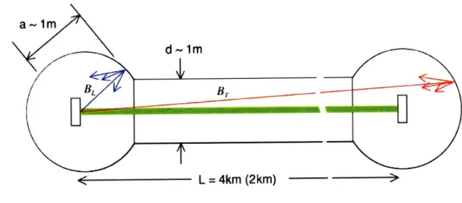
backscatter and baffle diffraction. Light can scatter off a LIGO mirror, backscatter off of a baffle, then return to the mirror and recombine with the optical beam. The theoretical spectrum of backscatter noise has been calculated by [8]. Likewise, when light scatters off a mirror it can defract off the edge of a baffle, back into the beam.

,<-

-L

= 4km (2km)

,

Figure 1-2: Light scatter in the interferometer arms. The two rectangles represent mirrors, and the green line represents the main beam. Current baffle geometry is designed to handle scatter at small angles (red), but large angle scatter (blue) turns out to be more than expected. Reproduced from [10].

Scatter off of baffles can be controlled in two ways. First, by selecting baffle materials that are highly black at the laser frequency, the overall magnitude of the scatter can be reduced. Second, by characterizing the way in which the material reflects light, the shape and orientation of baffles can be designed to minimize scatter back into the beam. The degree to which the reflection is specular, for instance, and the way the reflectance depends on the angle between the beam and the baffle.

Chapter 2

Theory of Optical Scattering

2.1

Smooth vs. Rough Surfaces

A "smooth" surface has a specular, or mirror-like, reflectance. The reflectance is highly non-uniform and depends on what solid angle is being considered. These surfaces exist due to the wave nature of light. If rough features of the surface are much smaller than the wavelength of incident light, those features appear smooth. Thus we define a smooth surface as having surface height variations that are small compared to incident light wavelength.

Fresnel predicted that reflectance from a smooth surface should only depend on the incident angle and the refractive index of the material. For nearly smooth surfaces, the reflectance can be approximated as[18]

e( ₎₂

R = F e oso) _(2.1)

where R is the actual reflectance, F is the Fresnel reflectance, o is the RMS roughness height, A is the wavelength of the incident light, and Oi is the angle of the incident beam from normal (as shown in Figure 2-1). Notice that a surface approaches the smooth limit in two cases: as a/A approaches zero, and as the angle of incidence approaches 90'.

direction gets scattered into the remaining hemisphere above the surface. At the opposite extreme, for very rough surfaces, the specular scatter is negligible. Rough surfaces are instead modeled using smooth lobes near the specular direction. There is no easy transition for materials between the two extremes. We find that the scattering behavior of such surfaces varies based on what angle they are illuminated and what reflected angle is being considered.

2.2

The BRDF

Nicodemus et al.[23] developed one standard for measuring the reflected scatter off a surface, the Bidirectional Reflectance Distribution Function, or BRDF. The BRDF incorporates information about the structural and optical properties of a surface, and thus is sensitive to both the wavelength of incident light as well as any surface or bulk contaminants. It is the standard measure of scatter that will be considered in this paper.

We can fully describe the reflected radiance LX at point p^ in direction x8 of a

surface using the BRDF[20]. Note that radiance is in units of radiant power per unit source area per unit solid angle.

LA( ,4 ) = BRDFA(, x., i) L,\(p,

•

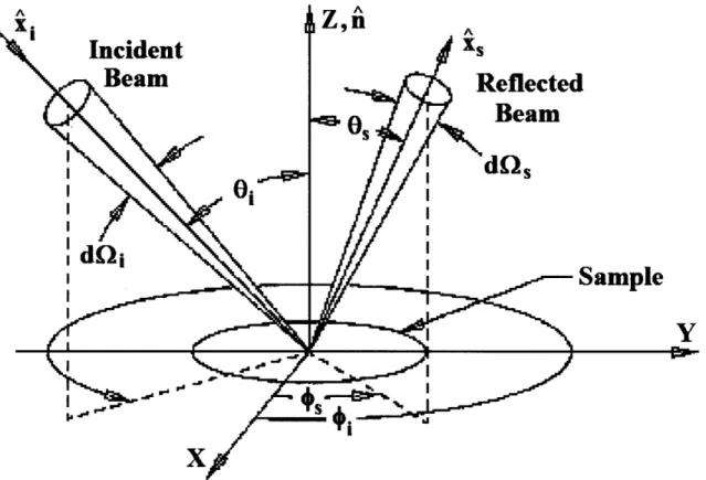
where LA(1, 4) describes the radiance incident on point P from direction Xi, d2i is the differential solid angle in direction x~, fi is the direction normal to the sample surface, and v is the set of all possible incident directions (the full hemisphere over the sample). Figure 2-1 illustrates the configuration of the beam and sample.

The BRDF function for a single wavelength can be expressed in terms of the reflected radiance and the incident irradiance, E(Xi), as

dL(xs) dPs/d(8

BRDF =- _(2.3)

dE(bi) Pi cos 0,

angle Q,. The cos O, factor adjusts the illuminated area to its apparent size in the

scattered direction. Irradiance is in units of power per unit area, and thus the BRDF is in units of 1/steradian. A

i

Incident

\

Beam

Zn

xs,

Reflected

Beam

Sample

Figure 2-1: Pictorial representation of the BRDF. Light reflecting off a surface in the X-Y plane. The BRDF relates the fraction of light reflected in direction i8 to the

incident power, Pi. Adapted from [5].

Because the BRDF is sensitive to surface and bulk contaminants, we must con-sider their effects in order to minimize their contribution to the measured value for black glass.

2.3

Surface Scatterers

Scatter from surface contaminants cannot be easily characterized. Because large particles create scatter patterns that depend on their size, shape, and constitution, there is no straightforward method to predict their behavior[23]. The total scatter can easily be dominated by contaminants, which can produce a BRDF several orders

of magnitude larger than the surface[3]. Dust particles have an average diameter of 1 ym, the scale of the LIGO laser wavelength[13]. By working under clean conditions, the contribution of these surface scatterers is greatly reduced.

The black glass was cleaned by drag wiping the surface with Lenx 90 tissue wetted with isopropyl alcohol. The surface was inspected visually for dust contaminants and streaking, and cleaned again if present.

Surface scratches also contaminant scatter. In order to minimize the influence of scratches and dust not visible to the naked eye, the BRDF was measured at three locations, each separated from the others by several centimeters. Contaminants on each location show up as patches of higher intensity that change intensity based on the angle of incident beam with the surface and the position of the beam relative to the contaminant.

2.4

Bulk Scatterers

Bulk scatterers are imperfections in the material, due to sub-surface contamination, damage, or other sources of inhomogeneity. While bulk effects are unlikely to be a dominant contamination source, they should be visible on a CCD image of the beam spot. Again, by measuring in multiple locations, we can account for these features.

Chapter 3

Previous Work

Previous studies[25] have utilized photodiodes to calculate baffle BRDF values. The results were found to be inconsistent because they could not distinguish contaminants and local surface defects from the material itself. By imaging the sample with a CCD camera, one can pick out the diffuse scatter, decreasing the BRDF by several orders of magnitude. Thus we can more accurately predict what the BRDF value should be in the clean conditions that are achievable in the vacuum environment of LIGO's arms.

Initial LIGO originally used oxidized stainless steel for baffles. Oxidized stainless steel has the advantages that it is sufficiently black at 1064 nm, the operational wavelength of LIGO, and it is relatively cheap to produce[6]. Unfortunately, it was discovered that the coating flaked within the vacuum beam tube, interfering with the

beam and with the vacuum quality[4].

The current baffle material preference for Advanced LIGO is black glass, a welder's glass manufactured by Schott. As of this work, the reflective properties of black glass

at 1064 nm were largely guessed at and a closer study was needed[22]. Concurrently with this work, another scatterometry arrangement has been designed and tested for black glass[16]. The results of this work will be compared to that one.

Chapter 4

Scatterometry Apparatus

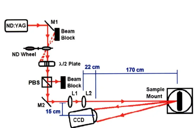
A schematic of the set-up can be seen in Figure 4-1. A Lightwave 126 series, 1064 nm ND:Yag laser[?] was used to illuminate the sample. A neutral density filter wheel as well as a A/2-wave plate and polarizing beam splitter combination allowed attenuation of the beam. Two mirrors guided the beam and two convex lenses were used to focus the beam down a long base line to the sample. The long base line minimized light pollution from the beam scattering off the optics.

A CCD camera placed next to the focusing optics, 1.70 meters from the sample, acted as the detector. The choice of camera proved to be a critical component of scatterometer. I used a Fuji IS-PRO digital camera, chosen for its sensitivity in the near Infrared, above 1000 nm[11]. The camera was set to manual mode with a shutterspeed of 1/50 s. Shaking due to touching the camera shutter button was greatly reduced by setting a timer delay of 10 s.

The IS-PRO can record images in a proprietary RAW format and in the Exif Version 2.2 JPEG file format. The JPEG format, set to 'fine' for a low compression ratio, was chosen for its portability. The process for calibrating the camera is discussed in the next section.

In order to measure the BRDF at multiple angles, I needed to design a sample mount that could rotate the sample in the plane of the optics table, while keeping the beam focused on the same spot. I constructed a mount from readily-available optical equipment that could rotate along an axis that runs through the sample. Figure 4-2

ND PBS M2 M1

Bealm

Bl oc k

Plate 22

Beam

Block

Figure 4-1: The scatterometry apparatus. A Nd:YAG laser is attenuated using a neutral density (ND) filter wheel before passing down a long baseline to the sample. The sample is imaged using a CCD camera placed near the incident beam. The half-wave plate and polarizing beam splitter (PBS) allow fine-tuning of the beam intensity.

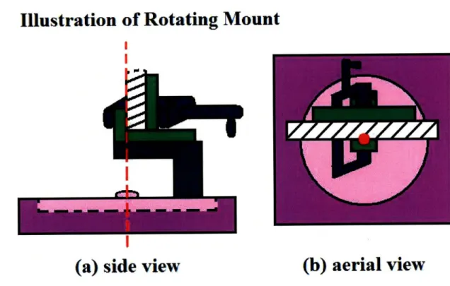
Illustration of Rotating Moun

I

(a) side view

(b) aerial view

Figure 4-2: The rotating mount. The sample can be clamped along the axis of rotation of the mount (red), allowing the same spot to be imaged at a range of angles. The mount consists of a rotating platform (purple), with an L-shaped post projecting over the axis of rotation (dark green). A second L-post is positioned so that the back of its lip aligns with the rotational axis (light green). The sample rests on this L-post, between the lip and a small platform (light green), which are used as surfaces that can be clamped in place (the clamp is blue).

illustrates the rotating mount.

The mount has a rotating platform as its base, with an L-shaped post attached to its rotating wheel. This post allows the sample to be positioned directly over the axis of rotation. A second L-post sits on top of the first, providing a lip for a clamp to rest against. A small platform placed against the back of the sample acts as a second surface for the clamp, fixing the sample in place. In order to take images over the size-scale of one beam waist, I created a second mount using a translational sliding platform.

it

Chapter 5

Measuring the BRDF

5.1

CCD Image Energy Level Calibration

The images produced by the CCD must be calibrated to real power units. This section lays out the process used to convert from the camera's machine units (mu) to Watts. The conversion requires two components: a prefactor, k, that converts from mu to W, and an exponential factor, y, that ensures the camera is linear over its range.

Most digital cameras record image intensity using an encoding gamma, which compresses the profile according to

Pc = p1 (5.1)

where Pc and Po represent the power of each pixel, normalized over the intensity range of the camera. The encoding ensures that images appear linear when viewed on a monitor. It also distorts the intensity map of the beam, and so it needs to be compensated for.

The first step to finding 7 and k was creating a reference image with a known

BRDF. Matt white paper has a Lambertian reflectance, and thus scatters uniformly.

The BRDF of a beam incident normal to a Lambertian surface has BRDF = . To convert between real intensity I(x, y) and CCD image intensity N(x', y'), the BRDF

relation is

BRDF = k(No(x', y')p2) 1

BRDF - (5.2)

I(x,y) (5

The image intensity No(x', y') is in [mu/pixel2_{], where the machine units have been}

gamma-corrected. The actual intensity, I(x, y), was measured in [W/mm2_{]. The}

pixels-per-millimeter conversion factor is denoted p. The solid angle of the camera lens, dQ, is given by

trD 2

d = L (5.3)

where D is the lens diameter and L is the distance between the lens and the sample. Because dG does not change between the calibration and the black glass measure-ments, it is incorporated into the conversion factor, k.

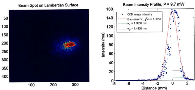
Before calibration, all images were imported into ImageJ[15], an image analysis program developed by the National Institutes of Health. The software has a useful image subtracting feature. By taking a dark image with the beam turned off, I was able to eliminate background light pollution. Each beam spot filled about 200 pixels squared-a small portion of the camera's total collecting area, but large enough to pick out features. See Figure 5-1 for a map of the beam spot. The corrected images were cropped around the beam spot and saved as text image files, then imported into Matlab for further analysis.

The second step in finding y and k is measuring the profile of the beam. I used an Ophir Model PD-300 series power meter[2] to measure the beam's integrated power

profile, Pr(x), using the razor method. Attaching a razor blade to a sensitive

transla-tional mount creates a beam block that can be slid across the power meter aperture. The power meter was positioned in the same location as the sample mount and exposed to the beam in increments, i. For a Gaussian beam, the total power as a function of exposed aperture is given by the integral of the two-dimensional Gaussian,

2P

00 x

2(X'

P(x) = 2P

M

Beam Intensity Profile, P = 9.7 mW

100 Zuu Juu -6 -4 -2

Distance (mm)

Figure 5-1: Left panel: Imaging the beam on a Lambertian surface. The map suggests some distortion in the x-direction. Laser speckle can clearly be seen. Right panel: A profile taken in the x-direction, through the peak intensity. The first beam waist,

wl comes from the fit to the integrated Gaussian described by Equation (5.5). The

second waist w2 was found from the Gaussian fit shown here.

P = 9.7 mW. Because the power meter is much larger than the beam spot, we can

approximate the the y-component integral limits as + 0o, which integrates to w -/2.

Integrating the x-direction integral gives the final expression,

P(x) = - 1 + erf .)) (5.5)

To compare the razor blade profile, P,(x), with the beam image, the image was transformed into a corresponding integrated power profile, No(x). The first step in finding No(x) is to crop the image to the region corresponding to the area measured by the power meter. To do this, I transformed the Pr(x) integrated profile into an intensity profile,

i Pr(xi+l) - Pr(xi) (5.6)

h(Xi+l - zi)

to find the location of the peak intensity. Here, h is the side length of the power meter. The peak intensity location, xi,, was designated to be the peak intensity location in the CCD image. If the peak is taken to be the zero point, the the CCD image range in the x-direction was chosen to correspond to -xi, as a lower bound

0 2

and h - xi. as an upper bound. The y-direction range was assumed to be symmetric

around the peak intensity. Figure 5-1 shows a plot of the beam profile through the peak intensity. The profile has been fit to a Gaussian curve. Deviation from Gaussian is visible, especially around the peak.

The next step in creating No(x) was passing the cropped image through a gamma decoder. The decoder applied a test value for gamma, -t, to the image,

Nt(x', y') = Nc(x', y') . (5.7)

After that, the image intensity in the y-direction was summed to create a linear profile,

hp

Nt(xi) = p2h Nt(x', y) (5.8)

j=1

For p in [pixels/mm] and h in mm, Nt(xi) is in machine units per millimeter, [mu/mm]. This can be converted to No,t(x) using

xp

No,t(x) = Nt(x - dx) + dx E Nt(xi) (5.9)

i=(x-dx)p

where dx is specified by each interval of the razor measurement.

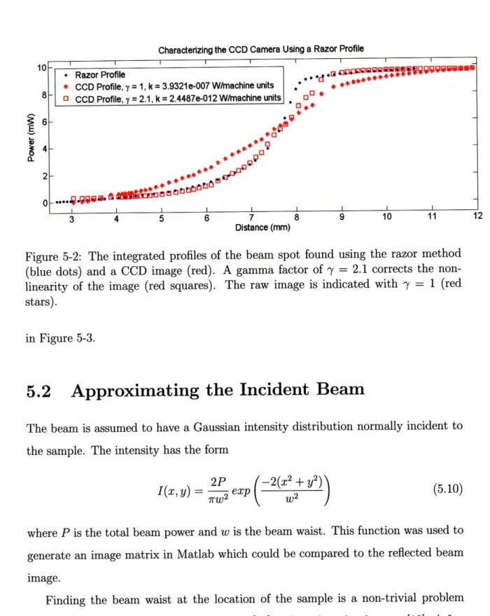
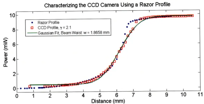
A X2/v-optimization between the CCD integrated profile, No,t(x), and the razor blade profile, Pr(x), was used to find the best-fit value for -. The integrated profile using the best-fit y was taken to be No(x). Figure 5-2 shows three integrated profiles. The razor blade profile (blue dots), a test integrated profile of the CCD image with

y = 1 (red stars), and the best-fit integrated profile of the CCD image with 7 = 2.1 (red squares). This is close to the NTSC standard, y = 2.2, which is also the y used to decode pictures on Windows operating systems. The 7 = 1 profile is shown in Figure 5-2 in order to illustrate that assuming a linear encoding for the camera does not corroborate with the razor blade profile.

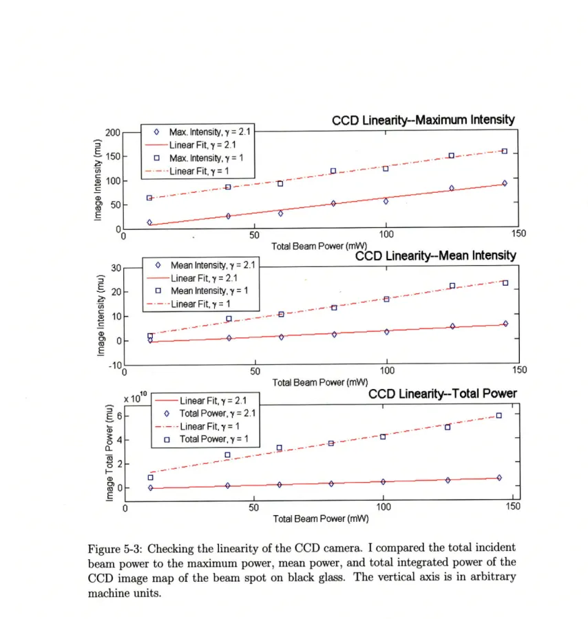
To test the linearity of the camera, I imaged beam spots on black glass over a range of incident power levels, from 10 mW to 150 mW. I checked the maximum power, mean power, and total integrated power of the image. The results are plotted

10 8 6 a-2 0

Characterizing the CCD Camera Using a Razor Profile

I I i I I I I I I

* Razor Profile .* ~ct imms 3,am

* CCD Profile, y = 1, k = 3.9321e-007 W/machine units " * **

o CCD Profile, y = 2.1, k = 2.4487e-012 W/hnachine units oD * o0 *

*

3 4 5 6 7 8 9 10 11 12

Distance (mm)

Figure 5-2: The integrated profiles of the beam spot found using the razor method (blue dots) and a CCD image (red). A gamma factor of y = 2.1 corrects the non-linearity of the image (red squares). The raw image is indicated with y = 1 (red stars).

in Figure 5-3.

5.2

Approximating the Incident Beam

The beam is assumed to have a Gaussian intensity distribution normally incident to the sample. The intensity has the form

I(x, y) = 2P e2x (5.10)

-irw w 2

where P is the total beam power and w is the beam waist. This function was used to generate an image matrix in Matlab which could be compared to the reflected beam image.

Finding the beam waist at the location of the sample is a non-trivial problem that has inspired methodological discussion[17] and product development[19]. A few methods were used to find an appropriate value.

The razor blade method is useful for finding a beam waist that corresponds to a prescribed power under the curve, regardless of the shape of the beam. Veshapidze,

et al.[12] have suggested that for a Gaussian beam, the beam waist can be more

I I .I __ I I __ I _ _I _ _

accurately measured by fitting the integrated profile, Pr(x), directly to Equation (5.5) rather than fitting the intensity calculated with Equation (5.6) to a one-dimensional Gaussian. From (5.5), we expect to measure

w = 2X84%P = - 2X16%P, (5.11)

where Z84% p means the position corresponding to 84% of the maximum power, P.

Equation (5.11) gave two values for the waist, 1.7 and 2.5 mm respectively. I determined the best value for w by doing a X2_{/v-optimization to Equation (5.5)}

using the measured Pr(x) profile and found a value between these two, w = 1.9 mm. Figure 5-1 shows the raw power with the Gaussian fit. Some non-Gaussian behavior is apparent from the fit, prompting the consideration of another measurement scheme.

Theoretically, we expect the beam width to increase with distance from the laser source, according to

w(z) = O 1 + (5.12)

where z is the distance in the direction of propagation and z0o is the Raleigh length,

defined by

zo = - (5.13)

Here, n is the refractive index of the propagation medium (in this case, air) and A is the wavelength of the laser.

When the beam is focused using a lens, the emerging beam has a new beam waist,

wO, located at distance d' from the lens. We can find w'o and d' using the following relations

wo' = wo f (5.14)

z

+

(d

f)

d' =

f

zd' 2 + (d- f)2 (

If we assume[7] the beam leaves the laser with wo = 0.1 mm, then we can use (5.14) and (5.15) to describe the beam incident on the first and second focusing optic, and then (5.12) to describe its propagation to the sample mount.

Unfortunately, the beam waist value is highly sensitive to the separation of the two focusing optics. I measured the separation to be about 75 mm. If w = 1.9 mm, the separation should be 69 mm, which is reasonably close, given that the optics are an inch in diameter.

In order to find p and convert between pixels and length, I imaged a 1 inch wide bar placed in the same location as the sample mount. Figure 5-5 shows the calibration image.

0 Max. Intensity, y = 2.1 - Linear Fit, y = 2.1

0 Max. Intensity, y = 1

-t--I inear Fit = 1

CCD

Linearity--Maximum Intensity

Total Beam Power (mW)

CCD

Linearity--Mean Intensity

CCD

Linearity--Total Power

100 150

Total Beam Power (mW)

Figure 5-3: Checking the linearity of the CCD camera. I compared the total incident beam power to the maximum power, mean power, and total integrated power of the CCD image map of the beam spot on black glass. The vertical axis is in arbitrary machine units. 200 150 1 100 0) 20 10 x io'10 E6 L_ a) O4 a) C0 EI

ED

3·'~'-1

Characterizing the CCD Camera Using a Razor Profile

I I I I I I I I I I

1 2 3 4 5 6

Distance (mm)

7 8 9 10 11

Figure 5-4: Finding the beam waist using the razor blade method. The blue points show the power measured by a power meter with partially exposed aperture. The red squares show the integrated profile measured by the CCD camera. The green line is the best fit of the CCD profile to an integrated Gaussian curve.

CCD Image of 1" Wide Bar Intensity Profile of Bar Ruler

60 1 _1 * Raw orfile 55, 850 pixels S45 S40 I 3 r-3U 25 20

A

'aI

VF

Figure 5-5: Converting pixels to length. Left: A 1" wide bar stood in the location of the sample mount. The yellow line indicates the slice of the image profiled to the right. The region in red corresponds to the width of the bar. Right: The intensity profile of the bar image, which clearly shows a sharp drop at the location of the bar. The error bars indicate the standard deviation in intensity among the columns highlighted in yellow in the left image.

2

* Razor Profile

O CCD Profile, ' = 2.1

- Gaussian Fit, Beam Waist: w = 1.8658 mm

I I I I I I I I I I 500 - 1000 o O 1500 2000 b5u 1000 1bU0 Distance (pixels) 2000 2000 E

[

0

Chapter 6

Near-Specular BRDF

6.1

Results

The CCD images of the beam spot on black glass were gamma-decoded, then corrected by k p2 from Equations 5.2 and 5.8 in order to convert from machine units to W mm-2

sr-_{'. I used Matlab to construct a Gaussian intensity map using Equation (5.10), in}

W mm-2_{. The total power incident on the black glass was P = 550 mW. A high}

power was necessary for large-angle measurements, discussed in the next section. A

BRDF map was created by dividing the reflected power by the incident power. This

way, the degree to which the BRDF varies over the image could be assessed, and surface contaminants accounted for. The map was made for a square area of diameter one beam width.

The BRDF for a near-specular angle of 3.30 was found to vary over several orders

of magnitude, typically from 1 x 10- s _{to 1 x 10}- 9 _sr- 1_{. The mode of the BRDF,}

however, remained fairly consistent for the three spot locations, on the order of 5 x 10-7 sr-1.

6.2

Surface Contaminants

As discussed previously, surface contaminants are illuminated by the incident beam in a way that is dependent on their structure and location. By translating the sample

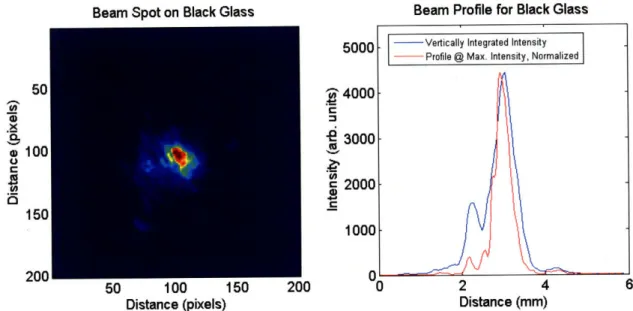
Beam Profile for Black Glass 0, -ii '3, Co C .0 'U co c U) c 0 5 1 00 1 50 200

Distance (pixels) Distance (mm)

Figure 6-1: Beam spot on black glass sample. Structure due to surface contaminants is visible. The red profile is a horizontal slice through the sample that runs through the maximum intensity. It has been normalized to the peak of the vertically integrated intensity (blue) for easier viewing.

in small fractions of one beam width, we can see their appearance change. This is neat to look at, and it confirms that the features of the beam spot are due to the

sample as opposed to the beam.

We can then check the extent to which each contaminant pollutes the BRDF. Contaminants consistently have BRDF values at least an order of magnitude higher than their surroundings, and often they have two orders of magnitude disparity. Be-cause the majority of pixels do not lie in regions with contaminants, we can look at the mode of the BRDF histogram to get a more accurate sense of the true BRDF.

6.3

Error Sources and Result Robustness

At the opposite end of the BRDF range are values up to an order of magnitude smaller than the mode. It is unclear to what extent these reflect the true BRDF. However a correlation exists between the picture quality and the abundance of low-valued pixels. Sufficient shaking in the camera smears the light intensity of one pixel over its neighbors, potentially creating regions of lower-than-true intensity (as well as

Beam Spot on Black Glass

Beam Spot, Position 3 I".t 12 10 .X 8 6 4 2

0-Position 1, Angle = 3.30 Position 2, Angle = 3.30 Position 3, Angle = 3.3"

I~l -14 12 10

8

BRDF, n, (lx10-n l/ster) BRDF, n, (1x10-n 1/ster) BRDF, n, (lx10n 1/ster)

Figure 6-2: BRDF for three spot locations on black glass. The distribution of the BRDF changes depending on the contaminants, but the mode remains fairly con-stant. The bars are color-coded according to order of magnitude. The mode for these histograms is on the order 5 x 10-7 and labeled in red.

regions of higher-than-true intensity).

It is worth considering whether or not using a Gaussian approximation for the incident beam is appropriate. Although the Gaussian fit was fairly good for the beam image on white paper (see Figure 5-1), the razor blade profile suggests some non-Gaussian features. In order to see what influence the beam waist had on the

BRDF distribution, I generated incident beam images over a range of w values, from

1.5 mm to 2.9 mm, which encompasses the range of w values found for different fit types. Figure 6-4 shows the mode of the resulting BRDF. The error bars indicate deviations in mode between the three spot locations. The deviation is less than an order of magnitude.

Beam Spot, Position 2 Beam Spot, Position 1

*"

,,,

Beam Spot, dx = 0.0635 mm

Figure 6-3: By varying the position of the black glass over spot, surface contaminants can be seen as regions of varying

jV IVV IU LVVUU LU

the width of one beam intensity.

BRDF Sensitivity to

Incident

Beam

Waist

1.4 1.6 1.8

2

2.2

2.4

Beam Waist (mm)

Figure 6-4: Varying the incident beam waist tests the sensitivity of the BRDF to small changes in beam waist, which suggests whether or not a Gaussian approximation for the incident beam is appropriate. The BRDF mode proved to be robust over a range of initial beam waist values. The BRDF remains on the order of 10- _{. The}

error bars indicate deviations in mode between the three spot locations.

III I I I I I T T 3EE I I 10-7

3.2

Beam Spot, dx = 0 mm _{Beam Spot, dx = 0.127 mm}

Chapter

7

Large-Angle BRDF

7.1

Results

In order to design baffles for Advanced LIGO, consideration must be given to how the BRDF behaves when the laser is incident over a range of angles from normal to the baffle surface (angle Oi from Figure 2-1). Using the rotational mount depicted in Figure 4-2, the BRDF for black glass was measured over a range of -50' through to 400.

I measured the BRDF for angles in both directions from specular in order to gain some perspective on the role contaminants could play in distorting the BRDF mode. The most significant difference between each direction of rotation is at 200, where the order of the BRDF varies by a factor of about 5 x 10- 1. After 300, the value for the cosine-corrected BRDF stayed consistently on the order of 10-', an order of magnitude smaller than the near-spectral value. Figure 7-1 plots the BRDF versus angle.

My results were consistent with those found by [16]. For comparison, Figure 7-2 shows the results in Figure 7-1 plotted against those of [16].

BRDF for Black Glass . I II I I U I I I I I I -50 -40 -30 -20 -10 0

Angle from Specular

10

(degrees)

20 30 40

Figure 7-1: BRDF for black glass. The angle of incidence was varied from -500 to

400 from normal to the sample.

BRDF Comparison

@

S-polarization

I Black Glass Trial 1

+ Black Glass Trial 2

N Black Glass, this paper

A A

A A

0 ... -- - - *

iu

Angle (degrees)

Figure 7-2: BRDF results compared to those from [16]. The method presented here agrees well. Plot adapted from [16].

-6 10-6 -7 10 U 1.E-01 1,E-02 S 1.E-03 11-05 , 1.E-06_-07 a 9 1.E-O0 . 1.E-06 1.E-07 • 1.E-08 ~----~ 10 .8 I I I I i I I I I

''dt

Chapter 8

Conclusions and Recommendations

Advanced LIGO promises to bring a new level of sensitivity to the LIGO interfer-ometers. In some frequency regimes, quantum noise will become the limiting factor. In order to reduce the amount of noise due to light scattering off the beam tubes and re-entering the main beam, baffles and beam dumps must be placed strategi-cally within the interferometer arms. Choosing a baffle material for Advanced LIGO that is highly black at 1064 nm will significantly reduce scatter noise. Characterizing potential materials will also inform the geometry and placement of baffles.

To these ends, I developed a scatterometer experiment designed to measure the Bidirectional Reflectance Distribution Function (BRDF) of a material sample. The

BRDF is a ratio of the reflected power per steradian to the incident power of the

beam. It encompasses surface properties of the material and how the material behaves when viewed from a range of angles. It is also sensitive to effects from surface and bulk contaminents and defects.

The scatterometer design has the advantage that it requires only components that could be found in most optics labs. The detector of choice was the Fuji IS PRO, which is sensitive at 1064 nm, the frequency used in LIGO interferometers. Imaging the beam spot on the sample with a CCD camera allowed me to view surface contaminants, which could inflate the BRDF by several orders of magnitude.

I used the scatterometer to measure the BRDF for black welder's glass, the prime candidate material for baffles in Advanced LIGO. I found that black glass has

a BRDF on the order of 10- 7 _{near-specular, and 10i} - _{starting at angles less than}

Bibliography

the gravitational wave. LIGO website, http://www.ligo.caltech.edu/LIGO_web/about/brochure.html, 2001.

[2] Pd300/pd300-1w/pd300-3w, photodiode detector head documentation. Ophir

[3] P A Carosso and N J P Corosso. Surface contamination monitoring by measure-ment of scattering distribution functions. Journal of Environ. Sci., 1987.

[4] H M Collins. Ligo becomes big science. Historical Studies in the Physical and

Biological Sciences, 33(2), 2003.

[5] Surface Optics Corporation. Surface optics web: Bidirectional reflectance distri-bution function, brdf, 2001.

[6] D C Coyne. Laser interferometer gravitational-wave observatory (ligo) project.

IEEE, 1996.

[7] Lightwave Electronics. 126 series, diode-pumped non-planar ring laser user's manual, 1995.

[8] E E Flanagan and K S Thorne. Noise due to backscatter off baffles, the nearby wall, and objects at the far end of the beam tube; and recommended actions. LIGO Technical Report LIGO-T940063-00-R, 1994.

[9] E E Flanagan and K S Thorne. Light scattering and baffle configuration for ligo. LIGO Technical Report LIGO-T950101-00-R, 1995.

[10] P Fritschel and M E Zucker. Wide-angle scatter from ligo arm cavities. LIGO Technical Report LIGO-T070089-05-D, 2007.

[11] Fujifilm. Digital camera is pro owner's manual, 2007.

[12] M H Shah G Veshapidze, M L Trachy and B D DePaola. Reducing the uncer-tainty in laser beam size measurement with a scanning edge method. Applied

Optics, 45(32), 2006.

[13] H E Bennet J M Elson and J M Bennet. Applied optics and optical engineering, volume 7. Academic Press, 1979.

[14] V Quetschke. Ligo -coherent optical length measurement with 10-18 m accuracy.

14th Coherent Laser Radar Conference, 2007.

[15] L Reinking. Imagej basics, version 1.38, 2007.

[16] D Riley and M Smith. Controlling light scatter in advanced ligo. LIGO Technical Report LIGO-T080064-00-D, 2008.

[17] C B Roundy. Current technology of laser beam profile measurements. Spiricon,

Inc, 1995.

[18] W H Li S H Westin and K E Torrance. A field guide to brdf models. SIGGRAPH

2004, 2004.

[19] N Savage. Laser-beam profilers. Nature Photonics, 1, 2007.

[20] C Schlick. An inexpensive brdf model for physically-based rendering. Computer

Graphics Forum, 13(3), 1994.

[21] D Sigg. Gravitational waves. LIGO Technical Report LIGO-P980007-00-D, 1998. [22] M Smith and P Fritschel. Aos: Stray light control (slc) design requirements.

LIGO Technical Report LIGO-T070061-02-D, 2007.

[23] J C Stover. Optical Scattering: Measurement and Analysis. SPIE Optical Engi-neering Press, 2 edition, 1995.

[24] K S Thorne. The scientific case for advanced ligo interferometers. LIGO Technical Report P-000024-00-D, 2001.

[25] M E Zucker. Comparison of video cameras for imaging diffuse scatter at 1064 nm wavelength. LIGO Technical Report LIGO-T990031-02-D, 1999.