On the direct identification of propagation modes for HF plasma waves

HAL Id: insu-03209854

https://hal-insu.archives-ouvertes.fr/insu-03209854

Submitted on 27 Apr 2021

HAL is a multi-disciplinary open access

archive for the deposit and dissemination of

sci-entific research documents, whether they are

pub-lished or not. The documents may come from

teaching and research institutions in France or

abroad, or from public or private research centers.

L’archive ouverte pluridisciplinaire HAL, est

destinée au dépôt et à la diffusion de documents

scientifiques de niveau recherche, publiés ou non,

émanant des établissements d’enseignement et de

recherche français ou étrangers, des laboratoires

publics ou privés.

On the direct identification of propagation modes for HF

plasma waves

Michel Parrot, François Lefeuvre, Y. Marouan

To cite this version:

Michel Parrot, François Lefeuvre, Y. Marouan. On the direct identification of propagation modes for

HF plasma waves. Journal of Geophysical Research, American Geophysical Union, 1989, 94 (A12),

pp.17049. �10.1029/JA094iA12p17049�. �insu-03209854�

JOURNAL OF GEOPHYSICAL RESEARCH, VOL. 94, NO. A12, PAGES 17,049-17,062, DECEMBER 1, 1989

On the Direct Identification of Propagation Modes for HF Plasma Waves

M. PARROT, F. LEFEUVRE, AND Y. MAROUAN

Laboratoire de Physique et Chimie de l'Environnement, Centre National de la Recherche Scientifique

Orleans, France

We examine the problem of interpreting the direct measurement of the polarization sense for HF plasma waves, in a cold and collisionless magnetoplasma when two propagation modes are simulta- neously present. Two types of propagation mode estimators are considered. The first, generally more sensitive to quasi-parallel waves, consists in the determination of the signs of cross-spectra between two electric or two magnetic wave field components, both perpendicular to each other and to B0. The second, more sensitive to quasi-perpendicular waves, is obtained by testing the ratio of the parallel to the perpendicular energy, against physical thresholds. Interpretations of the results are shown to be a function of the wave and plasma parameters. Applications performed on synthetic data constructed from two propagation mode models with different wave distribution functions (WDF) are presented. They show that the combination of the different propagation mode estimators often enables us to point out the presence of the two modes. Moreover, when the WDFs of the two modes are very different and when the wave frequency is far from the characteristic frequencies of the medium, the main propagation properties of each mode may be derived.

1. INTRODUCTION

The direct identification of the magnetoionic mode of high-latitude wave emissions is still controversial. As dis- cussed by Stix [1962], cold-plasma theory predicts four distinct electromagnetic modes of propagation at frequencies above the ion gyrofrequency. These modes are the free- space L-O mode (left-hand polarized, ordinary mode), the free-space R-X mode (right-hand polarized, extraordinary mode), the whistler mode, and the Z mode. With the exception of a few regions in the Clemmow-Mullaly-Allis (CMA) diagram, two modes may coexist [Stix, 1962; Allis e! al., 1963].

At present, the controversy is particularly strong as to the mode of auroral kilometric radiation (AKR). Because the radiation escapes freely from the Earth, it must be propa- gated in the free-space modes. Several polarization studies, mainly based on comparisons between the wave frequencies and the characteristic frequencies of the medium, conclude that the radiation is generated in the R-X mode [Gurnett and Green, 1978; Kaiser et al., 1978; Benson and Calvert, 1979]. However, Oya and Morioka [1983] have presented evidence that radiation is propagated in the L-O mode. One explana- tion proposed by Benson [1984] is that the R-X mode emanates from low-density cavities above the auroral re- gions and that the L-O mode is dominant in regions of relatively high electron density. Direct polarization measure- ments performed on DE 1, using orthogonal dipole electric antennas oriented such that, from time to time, they become perpendicular to the local magnetic field vector B 0, have pointed out the presence of R-X modes [Shawhan and Gurnett, 1982]. The detection of the L-O mode in other regions is obviously not excluded. The point is that the identification of the AKR wave mode in satellite wave

observations is important to the development of a correct theory for the AKR generation mechanism; for a review on AKR, see Grabbe [1981] and Oya and Morioka [1983].

As shown by Lefeuvre e! al. [1986], the mode that is

Copyright 1989 by the American Geophysical Union.

Paper number 89JA00743. 0148-0227/89/89JA-00743505.00

identified from electric or magnetic wave field component measurements is not always the one that conveys the max- imum wave energy density. Suppose that the L-O and the R-X modes are simultaneously present in the wave observa- tions presented by Shawhan and Gurnett [1982]. As the R-X mode gives the sense of polarization, one may be led to conclude that the R-X mode conveys the most energy. However, this may not be the case. According to Lefeuvre et al. [1986], the kind of estimators used by Shawhan and Gurnett, first, may be strongly biased in the vicinity of the critical frequencies, and so probably around the electron gyrofrequency where the AKR is supposed to be generated [de Feraudy et al., 1987], and, second, may favor the mode corresponding to waves having the wave normal direction K along the Earth's magnetic field B 0. Then, before interpret- ing polarization measurements, it is indispensable to evalu- ate the possible bias of the estimators and to find a way to check whether oblique waves propagating in the L-O mode are simultaneously present with the R-X mode or not.

The aim of the present paper is to give a general approach allowing us to answer these requirements. No hypothesis is made, a priori, about the distribution of the angle 0 between K and B0. The study is not restricted to AKR phenomena but is extended to all HF waves, i.e., to all waves with frequen- cies well above the proton gyrofrequency. The medium is supposed to be a cold collisionless magnetoplasma. In the absence of satellite data with more than three wave field

components, we have tested our ideas on synthetic data only. But the methods described here will find full applica- tions in future satellite missions such as Interball, where three magnetic wave field components and one electric field component will be transmitted to the ground in the HF range. Furthermore, they will be of prime importance in the design of future satellite missions when selecting which field components to measure and transmit to the ground.

The plan of the paper is as follows: Section 2 recaptures the dispersion relation and the characteristic frequencies of the medium. The wave distribution function (WDF) concept is used to evaluate the contribution to the sense of polariza- tion, when different waves modes are simultaneously present. It is shown that two polarization estimators (for

17,050 PARROT ET AL.: MODE IDENTIFICATION OF HF PLASMA WAVES

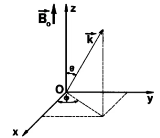
Fig. 1. Cartesian coordinate system used in the paper.

quasi-parallel and quasi-perpendicular waves) can give the polarization mode in the general case where the 0 distribu- tion is unknown. Examples of synthetic data are given. The validity domains and thresholds needed to compare to ex- perimental data are given in section 3. Section 4 offers some general conclusions.

2. ESTIMATORS OF THE POLARIZATION SENSE

The Dispersion Relations

A Cartesian coordinate system Oxyz (Figure 1) is as- sumed, in which the z axis lies along B o, the x axis is in the local magnetic meridian plane and points in the direction away from the Earth, and the y axis is oriented eastward. In this system, the wave normal direction K is characterized by the polar angle 0 and the azimuthal angle •b, as measured from the local magnetic meridian plane. Considering varia- tions of the electric and magnetic fields proportional to exp i(2•rft - K r), and taking •b = 0, the dispersion relation is expressed as

-iD

S-n 2

0

Ey

•n 2 cos

0 sin

0 0 P- n 2 sin

2

Ez/

-0 (1)

where n is the refractive index (n = kc/2•rf with c the velocity of light). The quantities S, D, and P are defined as by Stix [1962], but for frequencies well above the proton gyrofrequency they can be written

1

S = •.(R

+ L) D = •(R - L)

R=I-• L=I-•

f(f -- fce) f(f + fce)

P=I

where

fce and

fpe are the electron

gyrofrequency

and plasma

frequency.

The main types of electromagnetic plasma waves ob- served in high-latitude auroral regions are represented in the CMA diagram [Stix, 1962] in Figure 2. Since the wave frequency is high, the ion effect is negligible, and we do not consider regions above 8. The R-X mode is a fast extraordi-

nary mode, whose low-frequency cutoff is the R = 0 cutoff in the CMA diagram:

•fp

t•l

2 fce

fx

= '2

e

+ " + -•-

(2)

The low-frequency cutoff of the L-O mode is at the electron

plasma

frequency

fee, i.e., P = 0 in the CMA diagram.

The

Z mode is a slow extraordinary mode bounded by the upper hybrid resonance (S = 0 in the CMA diagram):

fUHR

= VJ•e + ./•e

(3)

and the L = 0 cutoff:

fz =

,2+

fce

(4)

The Z mode

radiation

may be a right-hand

(fpe/f < 1) or a

left-hand

(fpe/f > 1) polarized

mode. The whistler

mode

is

limited by either

fpe or fce, whichever

is smaller.

Other

representations of auroral wave emission can be seen in Figure 2 of Gurnett et al. [1983] and in Figures 3 and 4 of Grabbe [1981]. From the CMA diagrams in Figure 2, it is seen that the R-X mode and the L-O mode can coexist, as well as the L-O mode and the Z right-handed mode, or the Z

!eft-handed mode and the whistler mode.

The Use of the WDF Concept

Assuming that Oz is parallel to B 0 (Figure 1), the electric and magnetic wave field components are combined for the sake of convenience in a generalized electric vector e whose

components are

1,2,3 = Ex,y,z 84,5, 6 = Zoi•x,y,z (5)

with Z 0 being the wave impedance in free space. The WDF specifies how the wave energy is distributed relative to the two angles 0 and •b, the wave frequency f, and the propaga- tion mode rn (ordinary or extraordinary). It is written Fm( f, cos 0, •b) and defined as being everywhere nonnegative. [Storey and Lefeuvre, 1979]. At a given wave frequency f0, it is related to the autospectra and cross-power spectra of the six wave field components by the expression

So'(fo)

=-• Z

ao'm(fO

, COS

0, (•)Fm(fO,

COS

0, qb)do'

(6) The integral is taken over the surface of a unit sphere,

where do' = d cos 0 d•b is the solid-angle element. S ij is

either the autospectrum (i = j) or the cross-spectrum (i :• j)

between

the ei and ej components.

The coefficients

aum,

which are the kernels of the integral equations, are directly related to the corresponding autospectra and cross-spectra for an elementary plane wave in the magnetoionic mode rn. Their algebraic expression, derived from the Maxwell equa- tions, is given by Storey and Lefeuvre [ 1980]. They implicitly

depend

on the plasma

parameters

fpe and fce' The kernels

whose expressions are needed here are listed in the appen-

PARROT ET AL.' MODE IDENTIFICATION OF HF PLASMA WAVES 17,051 )-

R-X

mode

•7 s--o

•0

'

•0

,oo

L-O mode

2 _ 10- lie = a/Z- 1 O.1- 10-

Z mode

,oo

R L

whistler

mode

Fig. 2. CMA diagram from Stix [1962] with the main types of electromagnetic waves observed in the Earth's polar

magnetosphere and with negligible ion effect. Hatched areas represent (a) the R-X mode; (b) the L-O mode; (c) the Z

mode with right-hand polarization on the left off = fee and left-hand polarization on the right of f = fee' and (d) the

whistler mode.

Polarization Estimator for Quasi-Parallel Waves

Lefeuvre et al. [1986] pointed out that for quasi-parallel

waves,

the signs

of Ira (a12m)

and

(n 2 - S)/D are the same

in

most regions of the CMA diagram: positive for right-handed and negative for left-handed waves. However, in a few regions the situation is more complicated, as shown by Allis et al. [1963]. In the regions denoted 3 and 10 by Stix [1962]

(5 and 11 by Allis et at.), the quantity

(n 2 - S)/D has the

same sign for the two magnetoionic modes. This means that in those regions it is impossible to identify the propagation mode of a wave field from the cross-power spectral measure- ments of two electric components taken in a plane perpen- dicular to B0. In regions denoted 6-a and 12 by Stix (13 and 7-a by Allis et at.), the situation is even more complicated.

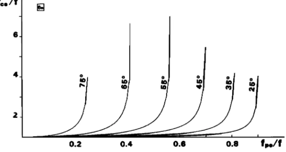
17,052 PARROT ET AL.: MODE IDENTIFICATION OF HF PLASMA WAVES f,:o/f 4 2 •,) 0 0 • 0 I 0 0 m m/ ml m m 0.2 0.4 O.e 0.8 f•e/f

Fig. 3. Representation of n 2 -- S in region 6-a of the CMA diagram (Stix) for different Oc values. When fce/f >> I the

asymptotic solution is given by cos 0 = ft, e/f.

angle

0c, given

by sin

20c = P/S. Examples

of Oc

values

in

region 6-a of the Stix diagram are displayed in Figure 3. For

n 2 < S to the right

of the figure,

it is impossible

to identify

the mode because the signs for the two modes are identical,

while

for n 2 > $ to the left, the R mode

as well as the L mode

can be distinguished. With the exception of the regions mentioned above, we obtain the relations for the cross-

power spectra of the two components of the electric field

orthogonal to B0:

Im (S•2) > 0 • R waves

(7) Im (S•2) < 0 • L waves

A null value is associated either with a linear polarization or with an equal contribution of the L and R waves to the sign of Im (S•2).

The sign of Im (a45m) also characterizes the polarization of quasi-parallel waves. It is the same as the sign of the quantity

(n 2 - $)P/[D(P - n • sin

2 0)]. Substituting

for !m (a45m)

in

(6), we get the relations for the cross-power spectra of the two components of the magnetic field orthogonal to Bo:

Im (S45) > 0 <-• R waves

(8) Im (S45) < 0 • L waves

which are independent of 0 [Marouan, 1988] and valid in all regions of the CMA diagram without any restriction. A null value is associated either with a linear polarization or with an equal contribution of the L and R waves to the sign of Im (S45).

One may evaluate the contribution of each mode to the

sign of Im (S•2) and Im (S45) by plotting Im (a12m) and Im

(a45 m) versus 0. One example was given in Figure 2 of Lefeuvre et al. [ 1986], and further examples are presented in Figure 4 for a range of plasma parameters. It can be observed that the estimators generally are more sensitive to small 0 values. In region 1 of the CMA diagram (Figure 4: panels A•, A3, B•, and B3), electric as well as magnetic components can be used to determine the sense of polariza-

tion. For the case shown in Figure 4, panels A• and B•, the

contributions of the R and L modes are approximately the same with a slight tendency to enhance the L mode. Unless

a very intense wave energy density is conveyed at large 0 waves, the sign of Im (a •) and Im (a45) is controlled by small 0 waves. The reader will note that in the R mode the Im (a•2m) coefficient is not null at 0 = 90 ø, which means that large 0 waves may contribute to the sign of Im (S•2).

For the case shown in panels A 3 and B3, the variation with 0 is completely different for the electric and the magnetic components. When considering first the magnetic ones, it can be seen that a large scale factor exists between Im (a45rn) in the L mode and in the R mode. The L mode is clearly dominant, with the consequence that unless the wave energy density in the L mode is negligible relative to the wave energy density in the R mode, it is the L mode only that contributes to the sign of Im (S45). In other words, it is practically impossible to detect the presence of the R mode when the two modes coexist. As far as the electric measure-

ments are concerned, the main point is the nearly constant value of Im (a•2m) in the R modes. At small 0 values the L mode is dominant, but as soon as 0 > 30 ø, only the R waves contribute to the sign of Im (S•2), and it becomes impossible to use the sign of Im (S•2) as an estimator of the sense of polarization for quasi-parallel waves.

The variations of Im (a45m) in region 3 of the CMA

diagram

are illustrated

in Figure

4, panel

B 4. At smaller

0

values the R mode is limited by resonance angle. Since Im (a•2m) cannot be used as an estimator in this region, as mentioned above, it has not been shown.

Two examples are given for region 6-a of the CMA diagram in Figure 4, panels B2 and Bs. Once more, only the magnetic estimator can be used. For the case of a low plasma frequency, shown in panel B2, a slight tendency exists to enhance the L mode, whereas for the case of a higher plasma frequency, shown in panel Bs, the L mode has clearly the more important contribution to the sign of Im (S45), at least for 0 values less than 50 ø. The reader will note that the maximum contribution of the R waves is at 0 = 30 ø and not at0=0 ø.

Polarization Estirnators for Quasi-Perpendicular Waves

Intuitively the polarization sense for perpendicular waves may be estimated from the quantities

PARROT ET AL..' MODE IDENTIFICATION OF HF PLASMA WAVES 17,053 177. 118. 69. 188. 126. 63.

IIm(.,,)••'--...•

f ,,/f =0.08

A.t

.•••••/f =0.9

,,,,,(.,•

f.,/f

=0.76

•LEFT

[Im(,,,•T'---...•

f ,,/f =0.08

B

2

Iom(",,•'•...•

f ,,/f =0.76

B

3

'•--'0.4

RIGHT

[Im(.,,,•)•

f ,,,/f =0.76

89.. '•/f =0.9

, , R

QH••..•

I

lem(',,•• f ,,/f =0.75

/f

=1.1

Fig. 4. Variations of the absolute values of Im (a12) and Im (a45) versus 0. The wave frequency is f = 300 kHz. We

have (Az and Bz) f•,e/f = 0.08 and fce/f = 0.9, (B2) f•,e/f = 0.08 and fce/f = 1.1, (A 3 and B3) f•,e/f = 0.75 and fce/f = 0.4, (B4)fpe/f = 0.75 andfce/f = 0.9, and (Bs)f•,e/f = 0.75 andfce/f = 1.1. In each panel, right-hand polarization and left-hand

polarization are considered. The units are arbitrary.

17,054 PARROT ET AL.' MODE IDENTIFICATION OF HF PLASMA WAVES

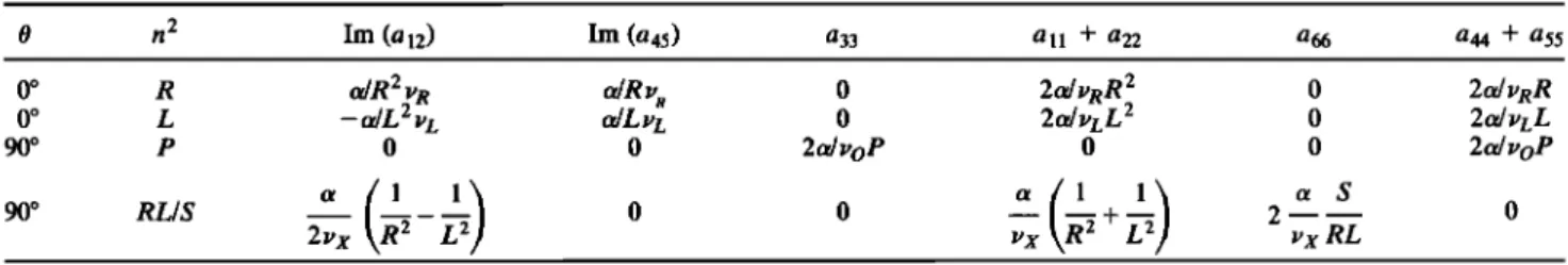
TABLE 1. Expressions of the Kernels of the Appendix in Special Cases

n 2 _{Im (a12) Im (a45) a33 all + a22} a66 a44 + a55

o 0 o 90 ø

90 ø RL/S

odR

2 vR

odR

v•

0

2Od

VR

R2

- odL 2 vL odL vœ 0 2Od VL L2

0 0 2OdvoP 0 2vx Vx 0 0 0 a S 2•• Vx RL 2 od vl• R 2od vœ L 2Od voP 0

Here a = l/e0 and vi = 1/2 to 3 {0/0•o [- (ton)-2]}i; i = R, L, O or X.

PE -- • 833 Sll + S22 (9) 866 S44 q- S55

which represent the ratios of the parallel to the perpendicular energy for the electric and magnetic wave fields. For 0-->

•r/2, Pœ -• oo

and PH --->

0 for O polarization

(n 2 --->

P),

whereas

P•r --> 0 and

PH--->

oo

for X polarization

(n 2 --->

RL/S).

In the following we will show that there are thresholds in PE and PH in certain cases allowing the identification of both the O and the X modes.

Consider first the following quantities: a33m(O) Pk( O)m = m= O, X allre(O) + a22m(O) (10) a66m(O) Ph( O)m = rn = O, X a44m(O) + a55m(O)

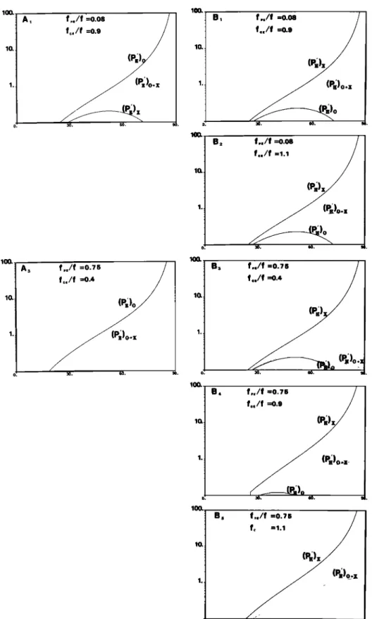
Examples of the functions P'(O)m are shown in Figure 5 (solid lines) for the wave and plasma parameters correspond- ing to Figure 4. Their characteristics can be understood with

the aid of the expressions

for aij listed

in Table 1, from which

it follows that P•r(O)x = P•r('rr/2)x = 0. With the exception of regions 3, 10, 6-a, and 12, discussed in the previous section, P•r(O)x is bounded by a maximum value Qœ at 0 = 0œ. Similarly for the magnetic components, Pb(O)o = Pb(•r/ 2) 0 = 0. In all regions of the CMA diagram, Pb(O) o is bounded by a maximum value QH at 0 = OH. Formally, Qœ

0_< 0_< •r/2

0_< 0_< •r/2

(11) and QH can be expressed as

Qœ = max [P•r(O)x]

max [Pb(O)o]

For the electric component of the O mode we find that P•r(O)o = 0 and P•r(•r/2) o = oo. Since the wave normal surfaces never cross, it follows that P•r(O)o > P•r(O)x for 0 -< 0 -< •r/2, again in all regions except the ones mentioned above. Similar arguments for the magnetic component of the X mode lead to Pb(O)x > Pb(O)o, which is valid in all regions.

A wave field may consist of both O mode and X mode. An example of the P values for a mixed wave field is shown with dotted lines in Figure 5. The field is composed of two WDFs

identical to Dirac distributions and centered on the same

value of 0. One WDF is the O mode, and the other the X

mode.

It can

be observed

that

the

P' functions

are

generally

more

sensitive to large 0 values. Region 1 of the CMA diagram is again the only one where electric as well as magnetic estimators can be used. For the case shown in Figure 5, panels A1 and B1, the electric and magnetic curves are quite similar, and P•rx and Pbo reach their maximum (=0.2) at 0 E = O H = 50 ø, whereas P•ro and Pbx are monotonic

functions that run from zero at 0 = 0 ø to oo at 0 = 90 ø. P•r(o+x) and Pb(o+x) are mean curves varying from 0 to 1. Referring

to the relations (11), we see that P•r > 0.2 indicates the presence of an O mode whereas P H > 0.2 identifies the presence of an X mode. It is likely that the hypothesis of a single propagating mode can be made for P•r or P H >> 0.2. The main contribution to the final value of the P•r and P H estimators is due to large 0 waves, one possible definition of the large 0 waves being 0 > 0•r, OH. For the case shown in Figure 5, panels A3 and B3, the situation is almost the same for PH, Pbo having a maximum =0.2 at OH = 52 ø. Due to the logarithmic scale, the P•x curve is not represented, but a threshold <0.01 may be adopted to point out the presence of the O mode (see Figure 11).

The situation in region 3 is illustrated in Figure 5, panel B4. There is a resonance angle for the X mode at 0 = 25 ø. The maximum of the Pbo curve is equal to =0.1 for OH = 40 ø. The two examples of region 6-a (panels B2 and Bs) have slightly different maxima, but do not present any particular- ity.

Returning to (11), it can be concluded that P•r values greater than Q•r indicate the presence of the O mode. The exact P•r value depends on 0 and on the wave energy density in each mode. In the same way, PH values greater than QH correspond to the presence of the X mode. On the other hand, a value of P•r less than Q•r, or of P H less than QH, cannot be readily interpreted since it may be due to parallel waves in any mode as well as to nonparallel waves in the X mode for Pe and in the O mode for P H.

The Mode Identification

Combining the results obtained for the quasi-parallel and quasi-perpendicular estimators, one generally obtains good information on the propagation mode present in the medium and on their propagation characteristics, without any hy- pothesis on the 0 distribution. This is illustrated in Figure 6 for two different values of the wave and plasma parameters.

The symbols (1[) and (_1_) represent quasi-parallel and quasi-

perpendicular propagation and are absent for propagation that is both parallel and perpendicular; Or is the resonance

angle

of the R-X mode at fpe/f = 0.75 and fce/f = 0.9. We

assume that in regions where they can be compared, there is no inconsistency between the signs of Im (S•2) and Im (S45). Obviously, simultaneous values of P•r and P H, such as

PARROT ET AL.' MODE IDENTIFICATION OF HF PLASMA WAVES 17,055 lOO. lO. A1 lOO. 2

_f,,/f

_=0.08

fc./f

=l.1

(P;)o.•

f,,/f =0.76

f.,/f

=0.4

f,,/f =0.76

f,/f =o.9

/•

_{f,,/f =0.76}

_/

f. =1.1

(P•)• ,

Fig. 5. Variations of (P•c)x, (P•c)o, (Pb)x, and (Pb)o versus 0 (solid line); (P•)x+o and (Pb)x+o (dotted line). The plasma parameters are the same as in Figure 4.

17,056 PARROT ET AL..' MODE IDENTIFICATION OF HF PLASMA WAVES fo./f = 0.08 ; f=./f = 0.9 • Im (S•) > 0 PH 0 Q. •

0 i•_x(//) R-x

Fig. 6. Identification of the propagation modes and the main propagation characteristics when combining the quasi-parallel and quasi-perpendicular estimations of polarization. In the top panel, Im

(S 0) means either Im (S]2) or Im (S45).

PE >> QE and PH >> QH, correspond to cases with two modes.

All these considerations being taken into account, it is observed that, provided the WDFs in each mode have different 0 distributions, one can make the distinction be- tween propagations in a single mode or in two modes, with indications on the general propagation characteristics: quasi- parallel or quasi-perpendicular. There are exceptions in cases with a dominant mode, i.e., when there is a large difference in the value of the Im (a12rn) and Im (a45rn) coefficients. In such cases there will always exist combina- tions of the sign of Im (S•2) and Im (S4•), and of the value of P• and PH, for which it is impossible to see whether the nondominant mode is present or not. The case of a dominant mode is discussed further in section 3.

The technique can be applied to experimental data. Know-

ing the plasma parameters fce and foe and the wave fre-

quency, one needs only to look to the sign of Im (S •2) and/or Im (S4•) and to calculate the ratios P• and/or PH. These ratios must be compared to thresholds evaluated as in (11). An example of the identification of the modes with synthetic data is given below.

Examples of Applications

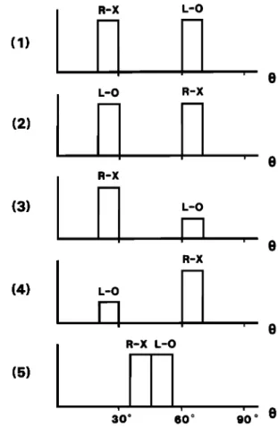
As an example of application, consider five different models of WDF (see Figure 7) where waves in the R-X and in the L-O modes are simultaneously present. For the sake of simplicity, it is assumed that the WDF in each mode is constant over a given 0 interval, the central 0 values of the WDFs being different for the two modes. No information on the ß distribution is needed since Im (a12m) and Im (a45m) are not • dependent. For each model, taking the plasma parameters of Figure 4, one obtains with (6) the values of Im [S•2(f)] and Im [S45(f)]. Then, applying (7) and (8), one estimates a propagation mode. The set of results is summa- rized in Table 2 a. In order to avoid too specific discussions, we have not considered the plasma parameters of Figure 4,

panel B4, for which a resonance angle has to be taken into

account.

The following two points come out:

1. For wave frequencies very close to a critical fre- quency (f = fx in panel B• of Figure 4) it is always the L-O mode which is identified, unless it has very little energy compared to the R-X mode, which is consistent with panel B3 of Figure 4, where the Im (a45) values in the R-X mode are always negligible in relation to the Im (a45) values in the L-O mode.

2. There is no simple rule to determine which waves have the most important contribution to the signs of Im (S•2) and Im (S4•).

The only way to improve our mode identification is to compute the values of the P• and P H estimators and to compare them to the Q• and QH thresholds. This has been done for the same conditions as above, substituting the five WDF models into (6). The QE and QH values are directly derived from Figure 5. The set of all relevant values is given

in Table 2b. The results of the tests are summarized in Table

2c. The dashes mean that P• < Q• or PH < QH. We note that (1) in most cases, P• and PH values of the order of 0.2 are high enough to detect the presence of a given mode, and (2) as forecast, P• values are used to point out the presence of one mode (here L-O) whereas PH values are used to point out the presence of the other mode (here R-X), the two measurements being sometimes complementary (model 5).

Now, examining Tables 2 a and 2c, we see that in most cases where electric and magnetic measurements can be compared (A• and B•, A3 and B3) one identifies the simul-

(1) (2) R-X L-O R-X L-O R-X (3) L-O (4) L-O R-X ' o R-X L-O (5) i

io o

e'o

o

,'o o e

Fig. 7. Models of WDF used for a test on synthetic data. The units are arbitrary.

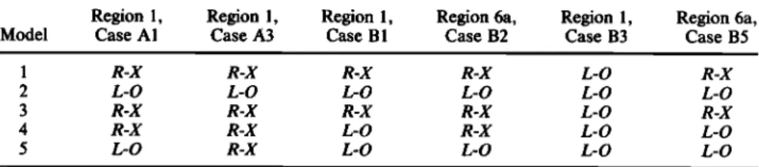
PARROT ET AL ' MODE IDENTIFICATION OF HF PLASMA WAVES 17,057 TABLE 2a. Results of the Test With Synthetic Data Obtained From Figure 7: Polarization

Estimator for Quasi-Parallel Waves

Region 1, Region 1, Region 1, Region 6a, Region 1, Region 6a,

Model Case AI Case A3 Case B I Case B2 Case B3 Case B5

I R-X R-X R-X R-X L-O R-X

2 L-O L-O L-O L-O L-O L-O

3 R-X R-X R-X R-X L-O R-X

4 R-X R-X L-O R-X L-O L-O

5 L-O R-X L-O L-O L-O L-O

The first two columns refer to panels Al and A 3 of Figure 4 obtained for electric measurements,

whereas the last four refer to panels B l to B5 of Figure 4, obtained for magnetic measurements.

taneous presence of the two modes. In all the other cases, where we rely on the magnetic data only, the full identifica-

tion depends on the sign of Im (S45). If it is negative, i.e., if it shows up the L-O mode, the PH estimator may point out

the presence of the R-X mode. If it is positive, i.e., if it corresponds to the R-X mode, it is not necessary to estimate the PH value any more: it does not contain any supplemen- tary information.

Returning to the ideal cases where magnetic plus electric data may be compared, most of the time one can obtain first approximations on the propagation characteristics in each mode. As an example, consider plasma parameters of panels A• and B• of Figures 4 and 5. Applying the strategy defined in

Figure

6 and

using

the signs

of Im (So.)

and

the

Pœ,

PH values

of Table 2, one observes that for model 1, the R-X mode is

conveyed by rather parallel waves and the L-O mode by rather perpendicular waves; model 2 is the opposite of model 1; the propagation characteristics of model 3 are similar to those of

model 1; the L-O mode of model 4 is not detected; and finally for model 5 we find L-O mode waves plus R-X mode waves propagating with K vectors nearly perpendicular to B 0.

An experimental illustration of the interest of a good definition of the Pœ threshold can be found in the Viking data

recorded by the V4H experiment [Bahnsen et al., 1987]. In

this experiment, the measured electric field component is alternatively almost parallel, then perpendicular to the geo-

magnetic field B 0. Then, assuming the wave field is time

stationary,

after half the spin

rotation

one may estimate

Pœ

(see equation (9)). This has been done for the event of Figure 1 of de Feraudy et al. [1987] just at the time (=2033 UT) where the satellite seems to pass through the source region of AKR emissions. Assuming that the plasma frequency is given by the upper cutoff frequency of the VLF hiss [de

Feraudy

et al., 1987]

we obtain

fpe = 20. kHz. As fce = 208

kHz, when

working

at f = 233 kHz, we have

fpe/f = 0.085

and fce/f-' 0.89, which is typically the case of our Figure 5,

panel A•. The computation of Pœ gives Pœ = 1.12. Referring

to Figure 5, panel A•, and equation (12), Pœ is compared against Qœ = 0.20. Our conclusion is that, as suggested by de

Feraudy et al. [1987], L-O mode waves are definitely present. Moreover, if we take the lower cutoff frequency of the event as well as the spin modulation pattern of the band as indicators of the presence of R-X mode waves, we find, with de Feraudy et al., that AKR emissions in the source regions are the sum of L-O and R-X mode waves. However, to be affirmative about the presence of R-X mode waves, one would need to estimate the quantities (7), (8), and (9).

3. THE VALIDITY DOMAINS

The Dominant Modes

To determine the wave and plasma parameters for which the quasi-parallel polarization estimators are strongly biased toward one of the two modes (see Figure 4, panel B3), we

define the quantities

g12 = Im [a12(O)]L Im [a12(O)]R (12) Im [a45(O)]L R45 = Im [a45(O)]R

For R•2 and R45 greater than 1 the L mode is called the

dominant mode, while for R •2 and R45 less than 1 the R mode is dominant. When one mode is dominant, the polarization

TABLE 2b. Results of the Test With Synthetic Data Obtained From Figure 7: Polarization

Estimator for Quasi-Perpendicular Waves

Case AI, Case A3, Case B l, Case B2, Case B3, Case B5,

Model

Q = 0.22

Q = 10

-3

Q = 0.22

Q = 0.12

Q = 0.21

Q = 0.10

17,058 PARROT ET AL.'. MODE IDENTIFICATION OF HF PLASMA WAVES

TABLE 2c. Results of the Test With Synthetic Data Obtained from Figure 7: Polarization Estimator for Quasi-Perpendicular Waves

Model Case A1 Case A3 Case B1 Case B2 Case B3 Case B5 1 L-O L-O ...

2 '" L-O R-X R-X '" R-X 3 L-O L-O ...

4 '" L-O R-X R-X R-X R-X

5 L-O L-O R-X R-X R-X R-X

The column heads refer to panels of Figure 5.

estimators tend to favor this mode although the other mode may be of larger energy density, thereby rendering the mode

identification difficult.

In order to study the behavior of R •2 and R45 for different

regions

of the CMA diagram,

the fpe/f ratio was fixed, and

the fce/f ratio was taken as variable.

Three

fpe/f values

are

considered' 0.08 (the left vertical line in Figure 2 a), 0.75 (the middle vertical line), and 1.2 (the right vertical line).

To have an idea of the 0 dependence, the computations of R•2 and R45 are done for one large 0 value (solid curve) and for one small 0 value (dashed line). Generally one takes 0 = 80 ø and 0 = 5 ø, respectively, but those values may be modified in regions with either a resonance angle Or or an

angle

Oc

for which

n 2 = S. The R•2 quantity

was estimated

even within regions of the CMA diagram where the identifi- cation of the propagation modes is impossible from the

electric measurements.

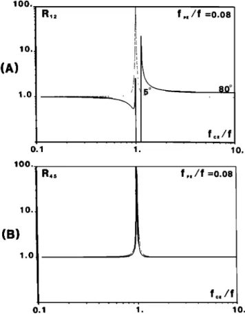
Figure 8a shows the variation of R 12 as a function Of fce/f

for fpe/f = 0.08. For R •2 > 1, there is a tendency

to observe

the left-handed polarized mode, even if the right-handed polarized mode has the same wave energy density; for R •2 <

1 the tendency is to observe the right-handed mode. As fce/f increases, one passes from region 1 in the CMA diagram to region 6 (regions 2 and 3 are not seen in the graph due to the

fpe/f value and the frequency

bin). In region 1 there is an

equal contribution of the two modes for fce/f • 0.3. When fce/f approaches 1, large 0 waves have a higher contribution

in the R-X mode than in the L-O mode, whereas low 0 waves show a higher contribution in the L-O mode close to fce/f-- 1 only. When f <fce, the L-O mode is greater than the Z right-handed mode, particularly for the large 0 waves. Note

that forfce/fvalues

between

1.0 and 1.123,

the quantity

n 2 -

S is negative at 0 - 80 ø, which means that no mode identification is possible, at least from the electric measure- ments. Figure 8b concerns the magnetic measurements (R45). The 0 - 5 ø and 0 - 80 ø solutions are practically identical, except in a very narrow domain around f =fce where the L-O mode is dominant above fce as well as below.

More important

effects

are seen

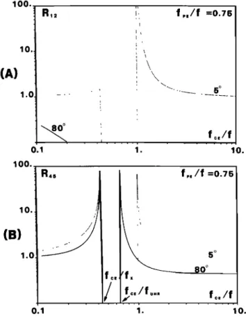
forfpe/f = 0.75 (Figure

9).

When the electric measurements are considered (Figure 9a), no mode identification is possible between the R = 0 cutoff (fx frequency) and the electron gyrofrequency with our method. This poses no problem for the interval between fx and fUI-IR (region 2 of the CMA diagram) since only one single mode propagates here. However, the interval between fUHR and fce corresponds to region 3, for which the interpre- tation of the sign of Im (S12) is ambiguous. For fce/f > 1, in region 6-a, the mode identification is again not possible up to a fce/f value given by 0 (see Figure 3). The latter constraint explains why there is no 0 = 80 ø curve below fce on the present graph. In any case, the interpretation of the sign of

Im (S•2) in this region of the CMA diagram is generally impossible since one does not know beforehand the position of the distribution in 0, with respect to the Oc angle. For fce/ f < 1, it is the mode with the highest wave energy that gives the sign of Im (S•2) if the waves propagate with small 0 values. But as soon as large 0 waves are present in the R-X mode (for instance, 0 > 30 ø at fce/f = 0.4 in Figure 4, panel B3), they control the sign of Im (S•2).

The mode identification is easier with magnetic measure- ments (Figure 9b). The L-O mode is dominant below fce/fx, the small 0 values being more sensitive to this mode. Above fce/fUHR the frequency domain for which the R45 curves may be drawn is a function of the 0 value under consideration. It starts from the vicinity of fce/fUHR for a large 0 value, but from fce/f • 1 for small 0 values. Although the interpretation is difficult, it is clear that at fce/f values below = 1.5 the L-O mode is dominant, whereas above this value it is the R-X

100. 10.

(A)

R,•

i f "/f

=0.08

(B)

Fig. 8. (a) Ratio between Im (a•2) in the L mode and Im (a •2) in

the R mode as a function offce/f, with fee/f = 0.08, f = 300 kHz. The

solid line corresponds to 0 = 80 ø, and the dashed line to 0 = 5 ø. (b) Same as Figure 8a, but for Im (a45).

fc,/f

PARROT ET AL.' MODE IDENTIFICATION OF HF PLASMA WAVES 17,059 mode. For fce/fvalues in between fce/fUHR and 1.0, there is

no propagation of small 0 waves due to the resonance angle.

Atfpe/f = 1.2 (Figure 10), a mode identification is required

for fce/f • 1 only (region 7). Due to the existence of a resonance angle the large 0 value has been fixed at 20 ø. The

solutions obtained for the electric measurements are dis-

played in Figure 10a. The left-handed polarized mode (Z mode here) is dominant over a large frequency domain. As far as the solutions obtained for the magnetic measurements are concerned (Figure 10b), they favor the Z mode just belowfce. At smaller frequencies, the Z mode is very slightly dominant for the largest 0 waves (which here are very small), whereas it is the whistler mode for the smallest 0 waves.

The Pœ and PH Thresholds

The variations of the PJrx and Pbo maximum values denoted QE and QH, respectively, as regards fce/f, are shown in Figure

11 forfpe/f= 0.08 (A l, B1), 0.75 (A 2, B2), and 1.2 (A 3, B3).

Note that the Q•r values have not been plotted in regions where the tests on the parallel to perpendicular energy of the electric field are not relevant. So one can consider that in the present field of study, electric and magnetic thresholds are always

below

-•0.6. At fixedfpe/fvalues,

they

both

decrease

whenfce/f

increases, and, conversely, at fixed fce/f value they both decrease when fpe/f increases.

In any case, one is very far from the constraints when assuming plane waves at 0 - 90 ø (Pe --> o• for the O mode and PH --> o• for the X mode). Values of P•r and PH greater than

100. 10.

(A)

=1.2

fc=/f

(B)

o. 1

... •.

lO.

Fig. 10. (a) Same as Figure 8a but for fpe/f = 1.2. The solid line

corresponds to 0 = 20 ø, and the dashed line to 0 = 5 ø. (b) Same as

Figure 10a but for Im (a45).

100. 10.

(A)

R,,5

I

f,./f =0.75

fc./fu.,

fc./f

(B)

Fig. 9. (a) Same as Figure 8b but forfpe/f = 0.75. The solid line

corresponds to 0 = 80 ø, and the dashed line to 0 = 5 ø. (b) Same as

Figure 8b but for fpe/f = 0.75.

a fraction of unity are sufficient to point out the presence of waves propagating in O or X modes.

As an indication, Figure 12 shows the variations of the and 0H angles; 0e values have not been plotted in regions where the polarization of the electric field is not readily interpretable. We see that the waves that contribute the most to the P•r and PH values always have 0 values above 70 ø for the magnetic measurements but they can also include waves

propagating

at 0 = 20

ø for the electric

measurements

(fpe/f -

1.2). The electric measurements, which were already found to provide a poor estimator of the polarization of quasi- parallel waves (see previous section), may also give rise to a poor estimator of the polarization of quasi-perpendicular

waves.

4. CONCLUSION

We have studied the problem of interpreting the direct measurements of polarization sense for HF plasma waves in a cold and collisionless magnetoplasma, in the case where two magnetoionic modes may simultaneously be present. It is shown that two types of propagation estimators could be considered.

The first estimator, generally more sensitive to the quasi- parallel waves, consists in the determination of the signs of Im (S•2) and Im (S45): the imaginary parts of measured cross-spectra between two electric or two magnetic wave field components, both perpendicular to each other and to the Earth magnetic field. According to the wave and plasma parameters at the point of measurement the estimator may

17,060 PARROT ET AL.' MODE IDENTIFICATION OF HF PLASMA WAVES QE o o.1 0.2 0.16 0.08.

e=0.08

•=0.75

I:.

f:e

f•e=l.2

f

f

ß

i

!z ß

f•

f•e

Fig. 11. Variations

of QE

and

Qiv

versusfce/fførfpe/f

= 0.08

(A], B1),fpe/f'-

0.75

(A2, B2),

anaft,

e/f = 1.2

(A3,

B3).

phenomenon may be so important at the vicinity of the

characteristic

frequencies

of the medium

(electron

gyrofre-

quency, upper hybrid frequency, R = 0 cutoff frequency, etc.) that the identification of a given mode may be impos- sible, even when it conveys the largest wave energy density.

The estimator used for the electric measurements (Im (S]2))

presents two serious drawbacks: first, it does not apply in

specific

regions

of the CMA diagram,

and second,

it may be

sensitive to quasi-perpendicular waves. There is no restric-

tion for the estimator used for the magnetic measurements (Im (S45)).

The second estimator, more sensitive to the quasi-

perpendicular

waves,

is obtained

by testing

the values

Pœ

and

P H of the ratio

of the parallel

to the perpendicular

energy,

in

the electric and magnetic wave field components, against thresholds. A major result of the study is the definition of

thresholds for electric as well as for magnetic measurements.

Their values, which depend on the wave and plasma parame-

ters, are always much lower than 1. For instance, with the parameters used for Figures 4 and 5, Pœ and PH values greater

than 0.2 are sufficient to establish the existence of O and X

PARROT ET AL.' MODE IDENTIFICATION OF HF PLASMA WAVES 17,061 0 ø

f-• =008

f....-=

o.76

1

•e lO

',

f-

f

f

Fig. 12. Variations of 0œand O H versus fce/ffOrfpe/f = 0.08 (A1, B1), 0.75 (A 2, B2), and 1.2 (A 3, B3). The wave

frequency is f = 300 kHz.

P H are not required. An example of application to Viking data

has enabled us to check that in the source region, AKR

emissions could be the sum of L-O and R-X waves.

Applications have been performed on synthetic data con- structed from two-propagation mode models with different wave distribution functions. They show that the combination

of the four estimators often enables us, to point out the

simultaneous

presence

of the two modes.'

Moreover,

when

the WDFs of the two modes are very different and when the wave frequency is far from the characteristic frequency of the medium, the main propagation characteristics in each

mode (propagation quasi-parallel or quasi-perpendicular) may be derived. But obviously there are cases where the use of the propagation mode estimators does not lead to reliable identifications. The only way to proceed is to perform a full determination of the WDFs in each mode, which has never been undertaken so far. As a consequence, if one wants to avoid any misinterpretations, one must carefully study the properties of the propagation mode estimators--as we did-- with the wave and plasma parameters in hand, before starting the analysis of real data.

17,062 PARROT ET AL.' MODE IDENTIFICATION OF HF PLASMA WAVES

wave field components of HF waves are not simultaneously recorded before being transmitted to the ground, it will not be possible to fully apply the techniques proposed here to real data. However, this will become possible in the near future with the Soviet Interball project.

APPENDIX

Here we give expressions

of the kernels

aij used

in this

paper, as a function of the plasma parameters.

(n 2 _ p)2

Im

(a12)

= n4(n

2

_ L)

2 (n

2

- S)Dx

(n 2_P)2cOs

2 0

P

n2(n

2 L)

2 (n

2- S)D 2

X

(n 2 - R) 2 cot

2 0

a33

=

n4

X

(n2-p)2(n2-R)2{1

1 }

2n

4

(n

2_R)

2+(n

2_L)• X

(n 2 - P)2(R - L) 2 sin

2 0

a66

--

4n2(n

2 - L)

2

X

a44

+ a55

= 2n2(n2

_ L)

2

ß {(P - L)2(n

2 - R) 2 + (P- R)2(n

2 - L)2}X

X = 8[E0I"g(A'

q- /•

(p

- L)2(n

2

- R)

2

}

A

'= 2(P-

R)

2 1

+ • •2-• • c0S2

0

(R - L) 2(n2

- P) 2

/x'

- (n

2

- L)

2 sin2

0

1 3

-2]

=

The Editor thanks T. Neubert, H. K. Wong, and a third referee for their assistance in evaluating this paper.

REFERENCES

Allis, W. P., S. J. Buchsbaum, and A. Bers, Waves in Anisotropic Plasmas, MIT Press, Cambridge, Mass., 1963.

Bahnsen, A., M. Jespersen, E. Ungstrup, and I. B. Iversen, Auroral hiss and kilometric radiation measured from the Viking satellite, Geophys. Res. Lett., 14, 471, 1987.

Benson, R. F., Ordinary mode auroral kilometric radiation, with harmonics, observed by ISIS 1, Radio $ci., 19, 543, 1984. Benson, R. F., and W. Calvert, ISIS 1 observations at the source of

auroral kilometric radiation, Geophys. Res. Lett., 6, 479, 1979. de Feraudy, H., B. M. Pedersen, A. Bahnsen, and M. Jespersen,

Viking observations of auroral kilometric radiation from the plasmasphere to night auroral oval source regions, Geophys. Res.

Lett., 14, 511, 1987.

Grabbe, C. L., Auroral kilometric radiation: A theoretical review, Rev. Geophys., 19, 627, 1981.

Gumett, D. A., and J. L. Green, On the polarization and origin of auroral kilometric radiation, J. Geophys. Res., 83,689, 1978. Gurnett, D. A., S. D. Shawhan, and R. R. Shaw, Auroral hiss, Z

mode radiation, and auroral kilometric radiation in the polar magnetosphere: DE 1 observations, J. Geophys. Res., 88, 329,

1983.

Kaiser, M. L., J. K. Alexander, A. C. Riddle, J. B. Pearce, and J. W. Warwick, Direct measurements by Voyager 1 and 2 of the polarization of terrestrial kilometric radiation, Geophys. Res.

Lett., 5,857, 1978.

Lefeuvre, F., Y. Marouan, M. Parrot, and J. L. Rauch, Rapid determination of the sense of polarization and propagation for random electromagnetic wave fields. Application to GEOS-1 and AUREOL-3 data, Ann. Geophys., $er. A, 4, 457, 1986. (Correc- tion, Ann. Geophys., $er. A, 5,251, 1987.)

Marouan, Y., Etats de polarisation et d6termination des caract6ris- tiques moyennes des ondes naturelies dans un magn6toplasma froid. Application h des donn6es EBF, Ph.D. thesis, Univ.

Orl6ans, Orl6ans, France, 1988.

Oya, H., and A. Morioka, Observational evidence of Z and L-O mode waves as the origin of auroral kilometric radiation from the Jikiken (EXOS-B) satellite, J. Geophys. Res., 88, 6189, 1983. Shawhan, S. D., and D. A. Gurnett, Polarization measurements of

auroral kilometric radiation by Dynamics Explorer-l, Geophys.

Res. Lett., 9, 913, 1982.

Stix, T. H., The Theory of Plasma Waves, McGraw-Hill, New

York, 1962.

Storey, L. R. O., and F. Lefeuvre, The analysis of 6-component measurements of a random electromagnetic wave field in a magnetoplasma, I, The direct problem, Geophys. J. R. Astron.

Soc., 56, 255, 1979.

Storey, L. R. O., and F. Lefeuvre, The analysis of 6-component measurements of a random electromagnetic wave field in a magnetoplasma, II, The integration kernels, Geophys. J. R.

Astron. Soc., 62, 173, 1980.

Acknowledgments. We thank H. de Feraudy for kindly provid- ing V4H data and for very informative discussions. We are obliged to A. Bahnsen, principal investigator of this experiment on Viking. Several points have been raised by the referees. We especially thank

one of them for his constructive criticisms that led to substantial

improvement of the paper.

F. Lefeuvre, Y. Marouan, and M. Parrot, LPCE/CNRS, 3A, Avenue de la Recherche Scientifique, 45071 Orl6ans Cedex 02,

France.

(Received May 20, 1987;

revised March 28, 1989'