Digital holographic imaging of aquatic species

(1)

Digital Holographic Imaging

of Aquatic Species

by

José Antonio Domínguez-Caballero

B.S., Instituto Tecnólogico de Morelia (2002)

Submitted to the Department of Mechanical Engineering

in partial ful…llment of the requirements for the degree of

Master of Science in Mechanical Engineering

at the

MASSACHUSETTS INSTITUTE OF TECHNOLOGY

February 2006

c Massachusetts Institute of Technology 2006. All rights reserved

The author hereby grants to Massachusetts Institute of Technology

permission to reproduce and

to distribute copies of this thesis document in whole or in part.

Signature of Author . . . .

Department of Mechanical Engineering

15 January 2006

Certi…ed by. . . .

George Barbastathis

Associate Professor of Mechanical Engineering

Thesis Supervisor

Accepted by . . . .

(2)

(3)

Digital Holographic Imaging

of Aquatic Species

by

José Antonio Domínguez-Caballero

Submitted to the Department of Mechanical Engineering on 15 January 2006, in partial ful…llment of the

requirements for the degree of

Master of Science in Mechanical Engineering

Abstract

The aim of this thesis is to design, develop and implement a digital holographic imaging (DHI) system, capable of capturing three-dimensional (3D) images of aquatic species. The images produced by this system are used in a non-intrusive manner to characterize the abundance, morphology and 3D location of the aquatic species. The DHI system op-erates by recording the hologram produced by the interference between a reference wave and the wave scatter by a coherently illuminated object with a charge-couple-device (CCD). The recorded hologram contains information about the amplitude and phase of the optical …eld as modi…ed by the object. This optical …eld is retrieved by numerical algorithms, which enable the reconstruction of the …eld at di¤erent distances relative to the detector from a single hologram. The recording of the holograms with the CCD allows the implementation of image post-processing techniques intended to enhance the recon-structed images. A description of the optimization of the reconstruction by means of an auto-scan algorithm and the reconstruction of large holograms are discussed. It is found that the in-line single-beam experimental set-up is the most suitable con…guration for underwater imaging of aquatic species. This is experimentally veri…ed by imaging brine shrimp and copepods under various conditions. Small, sub-10 m features of the objects were successfully resolved. It is also found that by using con…gurations with a spheri-cal reference wave, resolutions comparable to those obtained by a conventional optispheri-cal microscope can be achieved in a “lens-free” approach with larger working distances. Thesis Supervisor: George Barbastathis

(4)

Acknowledgments

I would like to thank my advisor, Professor George Barbastathis, for his guidance and support as well as for giving me the fantastic opportunity to work in his group. I have learned a lot from him in the past couple of years and I look forward to the years to come. Thank you for being such a great advisor.

I am also very grateful for the support, advice and energy that my co-advisors, Pro-fessor Jerome H. Milgram and ProPro-fessor Cabell Davis, have invested in this project.

I would like to thank all the members of the 3D Optical Systems Group not only for their help and advice, but also for their support and friendship. I have had a great time working with you guys.

Thanks to Anthony Nichol for helping me manufacture the high-pass Fourier …lter that I used in some experiments.

I am very thankful to Nick Loomis for helping me with the set-up of some experiments. Welcome to the amazing world of underwater digital holography!

Many thanks to Rebecca Moon for proof-reading this thesis. Thank you also for all your love and unconditional support.

Finally, I would like to thank my parents, Jose Antonio and Elsa, and my sister and brothers, Susana, Carlos and Javier, for all their love and support. It is this love that feeds me with energy to become a better person.

(5)

List of Tables

1.1 Categorization of acoustic systems. . . 14 4.1 Speci…cations of the selected diode laser. . . 88 4.2 Speci…cation of the Kodak KAF-16801E CCD. . . 93

(9)

List of Figures

1-1 Plankton net. . . 12

1-2 Copepod Eurytemora a¢ nis. . . 13

1-3 Acoustical sensing set-up for recording zooplankton. . . 14

1-4 Photo of an Acoustic Doppler Current Pro…ler. . . 15

1-5 Multi-frequency acoustic system. BIOMAPPER II. . . 17

1-6 Video Plankton Recorder. . . 18

1-7 Images of plankton taken by the VPR. . . 18

1-8 Underwater Video Pro…ler System. . . 19

1-9 The ZooVis System. . . 20

2-1 In-line recording setup for standard optical holography. . . 25

2-2 In-line reconstruction setup for conventional optical holography. . . 26

2-3 O¤-axis recording con…guration for conventional optical holography. . . . 27

2-4 O¤-axis reconstruction con…guration for conventional optical holography. 27 2-5 Coordinate system for holographic imaging system. . . 34

2-6 Scattering model for single object. . . 39

2-7 In-line single-beam recording set-up. . . 39

2-8 In-line Mach-Zehnder set-up: clean reference beam. . . 40

2-9 Modi…ed in-line Mach-Zehnder set-up with high-pass Fourier …lter. . . 41

2-10 Modi…ed in-line Mach-Zehnder set-up with variable attenuator. . . 42

2-11 In-line set-up with a spherical reference wave. . . 43

(10)

2-13 Example of an exact di¤raction kernel. . . 49

2-14 Example of a paraxial approximated di¤raction kernel. . . 50

2-15 PSF obtained experimentally. . . 51

2-16 Experimental set-up used to record the PSF of the system. . . 51

2-17 Transfer function from paraxial approximated di¤raction kernel. . . 53

2-18 Block diagram of the reconstruction algorithm by the convolution approach. 54 2-19 Reconstruction of the point source experiment. . . 55

3-1 1D model of the bandwidth for a hologram formation in a CCD. . . 58

3-2 Minimum allowable imaging distance for in-line holography. . . 61

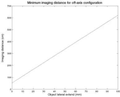
3-3 O¤-axis bandwidth model. . . 62

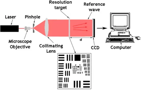
3-4 Minimum allowable imaging distance for the example of o¤-axis holography. 63 3-5 In-line set-up to measure the resolution limit in DHI. . . 65

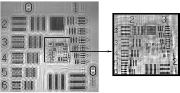
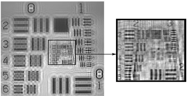
3-6 Image of a 1951 USAF resolution target reconstructed for d=12.5mm. . . 65

3-7 Image of a 1951 USAF resolution target reconstructed for d=286mm. . . 66

3-8 Image of a 1951 USAF resolution target reconstructed for d=600mm. . . 66

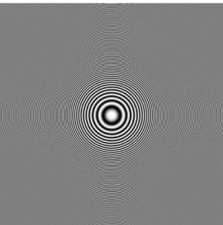
3-9 Hologram of the 1951 USAF resolution target. . . 68

4-1 Aberration produced by refractive index change. . . 74

4-2 Refraction from a ray emerging from a point source in seawater. . . 74

4-3 Spherical aberration produced by an on-axis point object. . . 75

4-4 Reconstruction of a resolution target: CCD properly aligned. . . 76

4-5 Reconstruction of a resolution target: CCD misaligned. . . 77

4-6 Optical absorption in seawater. . . 79

4-7 Output power after propagation in seawater: Pin=10mW. . . 80

4-8 Quantum e¢ ciency of the Kodak KAF-16801E CCD. . . 81

4-9 Minimum required laser power as a function of distance. . . 84

4-10 Minimum required laser power as a function of wavelength. . . 85

(11)

4-12 Minimum required laser power for Ti in the range [0.2msec,2msec]. . . 86

4-13 Number of bits versus laser power. . . 87

4-14 Number of bits versus propagation distance. . . 87

4-15 Number of bits versus integration time. . . 88

4-16 Interline-transfer architecture [87]. . . 91

4-17 Frame-transfer architecture [87]. . . 92

4-18 Full-frame transfer architecture [87]. . . 92

4-19 Object velocity versus integration time ranging from 100 sec to 3msec. . 95

4-20 Object velocity versus integration time ranging from 10 sec to 100 sec. 95 4-21 Monostable multivibrator circuit. . . 97

4-22 Time sequence from monostable multivibrator circuit. . . 97

4-23 In-line single-beam experimental set-up using a Helium-Neon laser. . . . 100

4-24 Hologram of a brine shrimp. . . 100

4-25 Reconstruction of a brine shrimp located 68mm from the CCD. . . 101

4-28 Reconstruction of a brine shrimp with a mild level of motion blur. . . 103

4-29 In-line single-beam experimental set-up using a Helium-Neon laser. . . . 104

4-30 Reconstruction of a brine shrimp using the entire CCD: d=103.5mm. . . 105

4-31 Reconstruction of a brine shrimp using the entire CCD: d=109mm. . . . 106

4-32 Comparison between recontructions using a portion and the full CCD. . . 106

4-33 Final in-line single-beam experimental set-up. . . 107

4-34 Final in-line single-beam experimental set-up: Top view. . . 108

4-35 Reconstruction of a brine shrimp using the …nal in-line single-beam set-up. 109 4-36 Reconstruction of a brine shrimp using the …nal in-line single-beam set-up. 109 4-37 Reconstruction of a brine shrimp at d=149mm. . . 110 4-38 Reconstruction of a brine shrimp using the in-line Mach-Zehnder set-up. 111

(12)

4-39 Reconstruction of a brine shrimp using the modi…ed in-line Mach-Zehnder

set-up with high-pass Fourier …lter. . . 112

4-40 Culturing tank for copepods. . . 114

4-41 Digital hologram of free-swimming copepods. . . 114

4-42 Reconstruction of a copepod using the in-line single-beam set-up. . . 115

4-45 Reconstruction of a copepod using the …nal in-line single-beam set-up. . 117

4-48 Reconstruction of a 1951 USAF resolution target using the experimental set-up with a spherical reference wave. . . 119

5-1 Reconstruction of large holograms algorithm: no storage to the hard drive. 122 5-2 Reconstruction of large holograms algorithm: storing the spectrum. . . . 123

5-3 Reconstruction of large holograms: storing the spectrum and reading the kernel from the hard drive. . . 123

5-4 Computational time versus the number of reconstructions. . . 124

5-5 Computational time for each iteration versus the number of reconstructions.124 5-6 Comparison between the original copepod hologram and two binary holo-grams with threshold = 40 and threshold = 50. . . 125

5-7 Histogram of the original copepod hologram. . . 126

5-8 Comparison between the original copepod hologram reconstruction and the reconstructions from the two binary holograms at d=114.4mm. . . . 127

5-9 Hologram of a copepod modi…ed by setting a portion to zero forming the letters “MIT” and its reconstruction. . . 127

5-10 Auto-scan reconstruction algorithm. . . 129

(13)

5-12 Hologram of copepods collected in the Boston’s Harbor on November 17th,

2005 at 1p.m. . . 131

5-13 Modi…ed hologram after the implementation of the block-averaging algo-rithm with a block size of 128 128 pixels. . . 131

5-14 Schematic of a reconstruction of a single plane. . . 132

5-15 Schematic of the instant-volume reconstruction algorithm. . . 133

5-16 Reconstruction performed by the instant-volume reconstruction algorithm from the modi…ed hologram of section 5.3.1. . . 134

5-17 Block diagram of the thresholding and analysis algorithm. . . 135

5-18 Binary image after thresholding. . . 136

5-19 Identi…ed ROI from the binary image. . . 136

5-20 Block diagram of the auto-focus algorithm. . . 137

5-21 Detection of the object’s axial position from a coarse scan. . . 138

5-22 Detection of the object’s axial position from an intermediate scan. . . 139

5-23 Detection of the object’s axial position from a …ne scan: step size = 0.1mm.140 5-24 Detection of the object’s axial position from a …ne scan: step size = 0.01mm.140 5-25 In-focus reconstructed image of a copepod at d = 40.25mm. . . 141

5-26 In-focus reconstructed images of copepods. From left to right, imaging distances: d= 62.5mm, d= 75mm and d = 69.5mm. . . 141

5-27 In-focus reconstructed images of copepods. From left to right, imaging distances: d= 73mm and d = 77mm. . . 142

5-28 Image processing sequence produced by the analysis algorithm. . . 143

5-29 Output Image from the analysis algorithm. . . 144

5-30 Hologram of a copepod and the modi…ed hologram with the DC term removed. . . 145

5-31 Reconstruction from original hologram and hologram with DC term removed.146 5-32 Phase distributions reconstructed from original hologram and hologram with DC term removed. . . 146

(14)

5-33 Modi…ed hologram and reconstruction obtained from high-pass …lter. . . 147 5-34 Modi…ed hologram and reconstruction obtained from Laplacian. . . 148 5-35 Band-pass …lter algorithm for DC term suppression. . . 149

(15)

Chapter 1 Introduction

1.1 Overview

In Chapter 1, the importance of studying aquatic ecosystems and the motivation to develop an instrument that facilitates the analysis and characterization of aquatic species is discussed. A brief overview of current technologies used to study plankton is also presented.

In Chapter 2, the concept of holographic imaging is described through the analysis of conventional optical holography. A more detailed examination of the foundation of digital holographic imaging (DHI) systems is explored through several recording set-ups and numerical reconstruction algorithms.

In Chapter 3, an analysis of the resolution of the DHI system and the sampling requirements is conducted.

In Chapter 4, design considerations required to develop the DHI system are addressed and experimental results from imaging brine shrimp and copepods are presented.

In Chapter 5, image post-processing algorithms designed to optimize, enhance and analyze the images obtained from the DHI system are described.

(16)

Chapter 6 provides a conclusion for the e¤ectiveness of a DHI system to characterize aquatic species based on experiments conducted with plankton. This chapter also sug-gests areas to further improve on the design, development and implementation of this imaging system and outlines future directions for this research.

1.2 Imaging of Aquatic Species

The critical need to understand the dynamics of aquatic ecosystems has led to the devel-opment of tools to help scientists collect high-resolution spatio-temporal data on species-speci…c population structures. Such data are critical for accurate modeling of biological populations towards a potential predictive capability of ecosystem ‡uctuations. In the case of aquatic (marine and freshwater) ecology, the implications of such ‡uctuations are re‡ected in issues such as: shoreline development; sewage and toxic pollution; over-…shing; and global warming. An ability to predict these issues would help governments and non-governmental organizations assess the impact of humans on the quality of their environment.

A signi…cant part of the research into aquatic ecology has been canalized to the analysis of planktonic populations. In the next subsections the importance of aquatic ecosystems and the roll of plankton will be brie‡y described in order to provide a basic understanding of the motivations in developing research in this …eld.

1.2.1 Importance of Aquatic Ecosystems

The earth is comprised of seventy-…ve percent water, of which ninety-eight percent is in oceans - where half of the earth’s photosynthesis occurs. A body of water principally constituted by multiple species interacting with each other and their chemical and physi-cal environment over multiple time-space sphysi-cales is considered to be an aquatic ecosystem.

(17)

From phytoplankton to small …sh and whales, the aquatic food chain constitutes a very complex system that still remains largely unexplored.

In aquatic ecosystems, plankton represents a fundamental link and constitutes the beginning of the food chain. Plankton is the aggregate community of swimming organisms that inhabit the water of oceans, seas, and bodies of freshwater. They are often used as indicators of environmental and aquatic health, due to their high sensitivity to changes in the environment, as well as for their short life span. Plankton can be divided into three broad functional groups:

Phytoplankton. These are algae that live near the water surface where there is enough sunlight to produce the photosynthesis required to survive. Phytoplankton are also called “producers” as they produce their own food.

Zooplankton. These are small protozoa, crustaceans and animals that feed on other plankton. Eggs and larvae of larger animals such as …sh, crustaceans and annelids are also included in this category.

Bacterioplankton. These are bacteria and archaea that are crucial to the absorp-tion of nutrients dissolved in the water.

Phytoplankton are great indicators of high nutrient conditions, due to their propensity to multiply rapidly if they are in adequate conditions. They also alter the biogeochemical cycling nutrients and carbon in the ocean. Similarly, zooplankton are useful indicators for the health of future …sheries, as they are the food source for many organisms of higher trophic levels.

Copepods are small aquatic animals that belong to the zooplankton subclass and con-stitute the largest and most diversi…ed group of crustaceans in the world. In addition, copepods include over 14,000 species, 2,300 genera and 210 families making them the dominant form of marine plankton and a fundamental part of the trophodynamics of the

(18)

ocean. From sponges to vertebrates, copepods can virtually parasitize or be the inter-mediate host of all animal groups, including mammalians and humans. In both marine and freshwater, copepods that parasitize …sh and gill are a serious pest of commercial importance. On the other hand, copepods also have the potential to act as control mech-anisms for malaria, by consuming mosquito larvae. Harmful Algal Blooms (HABs) can exert a dominant (and harmful) in‡uence on pelagic ecosystems via the consumption of nutrients, the production of toxins, and the creation of anoxic conditions [1].

The need to study planktonic populations and other forms of aquatic organisms has prompted a generation of sampling tools and techniques that provide some of the infor-mation required to understand the mechanisms of aquatic ecosystems. In the following subsection some of these sampling systems are brie‡y described.

1.2.2 Sampling Systems of Aquatic Species

Several sampling methods have been developed in order to better understand aquatic ecosystems. These sampling techniques can be broadly categorized into: direct sampling, acoustic sensing and optical imaging. The developed systems range from commercially available instruments, which are mass-produced, to one-of-a-kind instruments, produced for particular circumstances. Despite recent developments, most systems are still inad-equate for providing the high-resolution data on species abundances, morphology and life-stage needed to predict information including population sizes, species and habits. Acoustic techniques o¤er the possibility of longer range imaging, but they su¤er from a lack of speci…city and knowledge of the multidimensional features of the scattering functions. Optical methods o¤er a very high resolution and characterization of the ac-quired data, which is usually presented in a very convenient form for humans to analyze. However, optical techniques usually have a very limited sampling range, and if operated with high-powered light they disturb the animals being sampled, making it di¢ cult to capture their natural behavior.

(19)

Many of the systems made to characterize aquatic species have been devoted to the study of micronekton, nekton, and in particular the study of plankton. E¤orts to study the relationship of HABs to plankton were initially reported in [2] and [3]. These studies have also helped to understand the relationship between phytoplankton and zooplankton.

One of the techniques used often to analyze plankton is to capture small samples from the ocean with the help of “plankton nets”for a later characterization in the laboratory. Plankton nets are made of a very …ne nylon mesh supported by rings forming a truncated cone (similar to a wind sock) with a bottle attached to the narrower side. The net is towed through the ocean letting the water pass through the mesh but trapping small particles that are concentrated inside the bottle. An example of a commercial plankton net is shown in Figure 1-1 [4].

Figure 1-1: Plankton net.

This direct sampling technique produces the best morphological characterization of the species by imaging them in a controlled environment with high-magni…cation micro-scopes. However, plankton towing is highly intrusive and does not allow the behavior of the sampled organisms to be monitored. Information about the abundance as function

(20)

of location cannot be retrieved. An example of an image taken with a microscope from copepods collected using plankton nets is shown in Figure 1-2 [5].

Figure 1-2: Copepod Eurytemora a¢ nis. Female of 1mm in length, commonly found in estuarine waters throughout the northern hemisphere.

Acoustics techniques have proliferated considerably in recent years due to the ease of creating, recording and processing sound waves. Several reviews relating to contemporary instruments and sound scatter by organisms in the sea involving zooplankton have been written [6], [7]. Books describing the use of acoustics for …sheries assessments [8] and zooplankton acoustics [9] are also available.

The general set-up for acoustical sensing is shown in Figure 1-3. Acoustic sensors consist of a set of electronics for both transmitting and receiving the sonar signal. The transmitting electronics are connected to transducers that transform the electrical signal into a sound wave. The receiving electronics are connected to transducers that transform the pressure wave into an electrical signal that is then recorded and analyzed. For a more detailed explanation of the principles of sonar systems refer to [10] and [11].

There are two common methods used for sampling aquatic species: echo integration and echo counting. With echo integration the biomass is estimated by recording the backscattering of a sampled volume using either single frequency or multiple frequency

(21)

Figure 1-3: Acoustical sensing set-up for recording zooplankton.

inversions. With echo counting the number of organisms can be inferred from the multi-plicity of traces after recording the re‡ection of a single animal. When densities become high, echo counting presents problems due to multiple re‡ections that saturate the sys-tem and make individual traces indiscernible. More precise identi…cation of species may be accompanied with net tows or optical imaging methods.

One way to characterize acoustic sensing systems is to consider the number of beams and number of frequencies in which they operate. Table 1.1 contains a list of sensors categorized in this form [1]. Although many acoustical systems to monitor …sh are available today, the number of systems designed to monitor zooplankton are very limited.

Table 1.1: Categorization of acoustic systems.

Split Beam Dual Beam Single Beam Multi Beam

Single Commercial Commercial Commercial Commercial

Frequency FTV: Ja¤e [19]

Multiple Wiebe[12], [13] Wiebe [15] Maps/Taps: Not known

Frequency and Demer [14] Holliday [16]

and Gri¢ ths [17]

Wide band Not known Not known Commercial Not known

System (SciFish) Foote [18]

(22)

type. Many economical consumer oriented sensors for detecting …sh are available. Un-fortunately the lack of proper calibration procedures makes them unsuitable for scienti…c use as no quantitative biomass information can be retrieved. For this reason, the Acoustic Doppler Current Pro…ler (ADCP) is a very popular system in the oceanographic com-munity. This system works by sending four beams of sound into the water for a later measure of the Doppler shift and hence, some estimate of the vector-valued current (ap-pealing to estimate biomass) can be found. Studies of zooplankton biomass using this device were reported in [20]. Di¢ culties in achieving quantitative information made the ADCP a more suitable system for qualitative estimations of animal abundance. Figure 1-4 shows a photo of an ADCP [21].

Figure 1-4: Photo of an Acoustic Doppler Current Pro…ler.

Both dual beam and split beam systems have similar goals where the position of the animal must be known in order to estimate the incident sound intensity to discern the wave. These systems produce good quantitative measurements but they have to be calibrated routinely. In the dual beam system, the received and transmitted beam patterns are cylindrically symmetric and the ratio between the intensity of the received wave per object is used to locate the target and thus the target strength. In the split beam system, the disk is split into four quadrants sensitive to sound and the time delay between quadrants is used to distinguish the direction of the sound source. A comparison of the

(23)

performance of both systems can be found at [22], where split beam systems were found to be more robust in estimating animal positions. Current companies that manufacture bioacustic systems include Simrad, Reson A/S, Biosonics and Hydroacoustic Technology Inc.

Due to the low acoustic re‡ectivity of zooplankton, multi-beam systems provide higher power and larger …eld of view. The FishTV system [19] is one multi-beam system used to map the behavior of euphausiids and copepods.

The multi-frequency system is another type of acoustic sensor. A series of instruments in one frequency regime (400 kHz – 3Mhz) by Holliday [23] have been used in the past several decades to estimate the size and type of animals ranging from 200 m–1cm in size. The deployment of the latest version of the system, TAPST M _{is described in [16]}

where according to the authors, the best results were obtained at ranges up to 20 or 30m. Another example of a multi-frequency system is the Biomapper [12]. BIOMAPPER II is a newer version of this system fabricated by the Woods Hole group [24]. Figure 1-5 shows a sketch of the BIOMAPPER II [25]. Other examples of multi-frequency systems are found in [18] and [17].

The broadband system is the …nal type of acoustical sensors. An example of this sensor used in a laboratory can be found in [26]. A commercial broadband system is currently available from Scienti…c Fishery Systems Inc. [27].

The third type of sampling systems of aquatic species is the optical imaging systems. These systems have performed reasonably well for observing zooplankton and, in some situations; information regarding animal identi…cation and abundance can be retrieved. One disadvantage of these systems is that they tend to sample smaller volumes than acoustic systems. This is sometimes compensated by the use of fast frame rates and rapid surveys.

(24)

Figure 1-5: Multi-frequency acoustic system. BIOMAPPER II.

In the realm of optical imaging systems the Video Plankton Recorder (VPR) plays an important role, [28], [29]. The VPR is a video-microscope system that uses forward scattering light to image organisms that are nearly transparent ranging from 0.2 –20mm in size. Multiple cameras synchronized at 60 …elds per second (fps) to a red-…ltered 80Watts xenon strobe (pulse duration = 1 sec) image the same volume of water in order to provide information on di¤erent scales. The sampled volume ranges from about 1 ml to 1 l; depending on the settings of the magni…cation optics in each video camera. An au-tomatic image classi…cation system was developed, based on neural network approaches, to help reduce the vast quantity of data to a description of the patterns of concentration [30]. An example of a deployment of this device in the George’s Bank region can be found in [31]. Figure 1-6 shows the schema and photo of the VPR system. Images acquired using this device are shown in Figure 1-7.

The Underwater Video Pro…ler System is an alternative imaging device capable of sampling organisms down to 100 m in size [32]. It consists of a Hi-8 video camera, a

(25)

Figure 1-6: Video Plankton Recorder. To the left: the schema of the VPR showing the layout of mayor components. To the right: the VPR tested at the Woods Hole Oceanographic Institute. (Photo by Woods Hole Oceanographic Institute)

Figure 1-7: Images of plankton taken by the VPR during transatlantic survey in August 2003. (Photo by Woods Hole Oceanographic Institute)

(26)

controlling and logging unit, batteries and several light systems. The lighting system can either consist of four spotlights to illuminate a volume of 70 l of water, or be a collimated light …eld in front of the camera that produces an illumination sheet used for particle distributions. Results of some deployments of this system can be found in [33], [34] and [35]. Figure 1-8 shows a photo of an Underwater Video Pro…ler System [36].

Figure 1-8: Underwater Video Pro…ler System.

The ZooVis System is an alternative optical imaging system design to collect quan-titative images of zooplankton to depths of 250m [37]. The system is based on a high-resolution camera pointing down into a sheet of light produced by a strobe. The strobe and the camera are synchronized to take images with su¢ cient quality to di¤erentiate between species. The ZooVis System is shown in Figure 1-9 [38].

The 3D Zooplankton Observatory is a system designed to obtain information about three-dimensional trajectories of zooplankton using Schlieren imaging in conjunction with multiple cameras to obtain orthogonal projections of the target [39]. The system images 1 l of water and permits viewing aquatic organisms ranging from phytoplankton to …sh. An alternative device to image organisms under water is the Flow Cam system by

(27)

Figure 1-9: The ZooVis System.

Fluid Imaging Technologies, (Boothbay, ME). The Flow Cam system works by pumping samples through a small illuminated volume that has high-resolution optics incident upon it. The system is optimized due to the small size of the volume of interrogation. However, this limits the system to be used in situ.

FIDO- is an imaging system design to map the location and biomass of phytoplank-ton by recording the scattered or ‡uorescent light from a volume of approximately half a liter. In a typical application, the volume of water is illuminated with a sheet of light allowing imaging of an area of 25cm x 25cm at a range of 80cm [40], [41].

An optical imaging system of speci…c interest to this thesis is underwater holography. In the standard form, holographic imaging uses a photosensitive …lm to capture the interference pattern between a reference wave and the wave scattered by an illuminated object. In-line and o¤-axis are the two main con…gurations that can be encountered. In in-line con…guration, both the object and reference wave are collinear and parallel to the optical axis of the recording medium. In the o¤-axis con…guration, the two beams are

(28)

separated by a small angle producing a di¤erent e¤ect during the reconstruction of the target. Information about the amplitude and phase of the object …eld can be retrieved by illuminating the recorded …lm with a beam similar to the reference beam used in the recording step. The details of this method will be explained in the next chapter.

Holographic imaging of underwater organisms is a particularly e¤ective technique as it provides a good characterization of the morphology of the animals and recovers their three-dimensional location. By capturing several consecutive holograms, data regarding biomass and ‡ow type can be retrieved. A good review of the principles and practice of holographic recording of plankton can be found in [42].

It is important to note that there are other systems available to count plankton including the optical plankton counter (OPC) and the laser optical plankton counter (LOPC). As these systems are not considered "imaging systems" per se, they have not been discussed in this section. The main reason they are not considered imaging systems is that they do not produce representations (or images) of physical objects. These systems are design to count the number of objects of interest per unit volume.

Hybrid systems (combining acoustics and optics) have been developed in order to compensate the limitations that occur with the individual systems. The lower frequency acoustical techniques for sensing zooplankton are advantageous in mapping moderate distances (10’s-100’s of meters) and the optical systems are more e¤ective for animal identi…cation. Examples of in situ hybrid systems are documented in [43] and [44].

1.3 Motivation for Digital Holographic Imaging of

Aquatic Species

In the previous section, the importance of studying aquatic ecosystems and a survey of the current sampling methods for plankton were discussed. None of these techniques

(29)

rep-resents an optimum solution to the problem of underwater species characterization. In order to develop a predictive capability in environmental science, it is imperative to ac-quire data relating to biomass, behavior, morphology, and the life stage of the organisms that inhabit a certain aquatic ecosystem. Although acoustic sampling methods gener-ally provide high-resolution backscatter data for estimating abundance concentrations, they do not provide detailed information regarding size and taxonomical composition of plankton. Optical techniques have been shown to produce better results in the level of species identi…cation, but tend to sample smaller volumes of water and therefore re-quire faster surveys to compensate. In addition, most devices are very bulky and, due to their short sampling range, disturb the animals that are sensitive to hydrodynamic disturbances. This invasiveness a¤ects mapping the true behavior of the organism under study. Optical imaging systems that work with high-powered light, such as the Video Plankton Recorder (VPR), produce an additional disturbance to the natural dynamics of plankton.

Digital Holographic Imaging (DHI) is a technology promising to solve the majority of the problems identi…ed. With DHI, the morphology of the sampled objects can be retrieved with su¢ cient quality to estimate the size, life stage and correspondent species. In addition, the three-dimensional position relative to the imaging sensor can be com-puted from a single captured image (single hologram). In the basic con…guration, DHI is a lens-free technique that is capable of sampling large volumes from a single hologram by means of post-processing digital scans, allowing estimates of the biomass concentrations. The highly sampled range provided by this method, assuming that the water is su¢ -ciently clear, allows a non-intrusive system to map the natural behavior of the animals being studied. By capturing consecutive holograms along the path of an underwater vehicle it is possible to estimate trajectories and swimming velocities of plankton.

DHI records the hologram in a CCD that usually requires low levels of coherent illumination. No …lm is used; therefore, no chemical post-processing is required to retrieve

(30)

the recorded optical …eld. As the image is already available in digital form, several image post-processing algorithms can be applied to reconstruct and enhance the quality of the image. Automatic plankton categorization algorithms can be implemented to help reduce the amount of computation. DHI systems for aquatic species can be built in a very compact form allowing ‡exibility of manipulation and a reduction of the hydrodynamic disturbances that a¤ect plankton. In the past few years, technologies such as CCD imaging sensors, computers and pulsed diode lasers have been showing technological progress that are further favorable for practical underwater DHI.

The goal of this thesis is to describe the characterization, design and implementation of a digital holographic imaging system for aquatic species. This imaging system is part of a larger project, with the ultimate goal of developing a system capable of sampling all aquatic regions on earth, including the full depth of the ocean (11,000m). An Autonomous Underwater Vehicle (AUV) will carry the DHI system. In order to obtain a better characterization of the aquatic ecosystem, the AUV will also be equipped with additional sensors. Multiple AUVs working simultaneously in a given region would provide the high-resolution species-speci…c abundance data needed for accurate environmental modeling, assessment, and prediction.

In the next chapter, the basic principles and formulations of digital holographic imag-ing will be discussed.

(31)

Chapter 2 Digital Holographic Imaging

2.1 Conventional Optical Holography

In 1948 Dennis Gabor invented optical holography. This invention, for which he won the Nobel Prize for Physics in 1971, was a result of an “exercise in serendipity”, as Gabor explains in his autobiography. Optical holography was initially presented in the context of electron microscopy as a method to resolve the problem introduced by the spherical aberrations of electron lenses that set the limit in the resolving power [45]. Two detailed papers, [46], [47], followed his pioneering work, which explored presenting holography as a method for recording and reconstructing the amplitude and phase of a wave …eld. He invented the world “holography” from the Greek words “holos” meaning “whole” and “graphein”meaning “to write”. Holography only attracted mild interest until the 1960s, when the concept became popular, improved predominantly by the invention of the laser. A hologram is a recorded interference pattern formed by combining a …eld scattered by a coherently illuminated object, with a …eld from background illumination (termed a reference wave,) which must be mutually coherent with the object-scattered …eld. In the conventional form, the interference pattern is recorded on a photosensitive …lm that is chemically developed later. The information about the 3D wave …eld scattered by the

(32)

object is encoded into a set of fringes (interference fringes). This set of fringes is usually not visible to the human eye due to the high frequency content. The 3D object wave is reconstructed by illuminating the …lm again with the reference wave. In experiments conducted by Gabor both the reference wave and the object wave were collinear and normal to the photographic plate. This con…guration is known as “in-line” where the reconstruction results in the real image being superimposed by the undi¤racted part of the reconstruction wave (the DC term) and the virtual image. This con…guration is explained in greater depth later in section 2.2. Figure 2-1 shows a sketch of a typical in-line recording setup. The reconstruction setup is shown in Figure 2-2.

Figure 2-1: In-line recording setup for standard optical holography.

The application of the Gabor hologram is bound by certain limitations. One sig-ni…cant limitation is the assumption of imaging highly transparent objects. The e¤ect of removing this assumption is discussed in more detail in the next chapter, where the quality of the holograms is analyzed in relation to the number of particles being imaged (in other words, the transparency of the object). Another signi…cant limitation is the overlapping between the twin-images (virtual and real images) and the DC term. Several

(33)

Figure 2-2: In-line reconstruction setup for conventional optical holography.

methods have been developed to overcome these limitations including the earlier work by Gabor [48] and the more recent phase-shifting techniques [49].

Leith and Upatnieks made signi…cant advancements on Gabor’s technique by in-venting o¤-axis holography [50], [51]. Whilst conducting research at the University of Michigan’s Radar Laboratory, they observed the similarity between Gabor’s lens-less imaging system and the synthetic-aperture-radar problem. In o¤-axis holography, the interference pattern is recorded with a reference wave tilted by a small angle respective to the optical axis as shown in Figure 2-3. The small angular di¤erence is equivalent to the use of heterodyning in radar, which was Leith and Upatnieks’inspiration. The main advantage of o¤-axis holography is that the DC term and the real and virtual images are spatially separated during the reconstruction. However, the high-frequency content of the hologram sets a limit in the type of recording …lm required in the experiment. Figure 2-4 shows the o¤-axis reconstruction setup.

As noted earlier, most recordings performed in optical holography are made on a photographic …lm or plate. The …lm used to record the interference pattern is assumed to provide a linear mapping of intensity incident during the detection process into amplitude

(34)

Figure 2-3: O¤-axis recording con…guration for conventional optical holography.

(35)

transmitted by or re‡ected from the …lm during the reconstruction process [52]. Several other materials suitable for holography also exist, including photorefractive materials, dichromated gelatin and photopolymers.

During the same period that Leith and Upatnieks were developing o¤-axis hologra-phy, Y.N. Denisyuk, a scientist from what was then the Soviet Union, invented the thick re‡ection hologram. This hologram was greatly in‡uenced by the work of Gabor and G. Lippmann [53], a French physicist. With re‡ection holograms, there is only one illumi-nation beam working as a reference and illuminates the object through the holographic plate.

Holograms are sometimes also classi…ed by the di¤raction or imaging conditions that exist between the object and the recording medium. The …rst classi…cation is the Fresnel type. A hologram is considered to be of this type if the recording plane lies within the region of Fresnel di¤raction of the illuminated object. As expected, the second class is the Fraunhofer type. With this type of hologram, the transformation from the object to the recording plane is better described by the Fraunhofer di¤raction equation. A hologram is referred to as an image hologram if the …lm is located in the image plane of the optical system. In the case of Fourier holograms, the recording plane resides in the Fourier plane of the object amplitude transmittance. Finally, with the lens-less Fourier transform hologram, the reference wave comes to focus in the object plane and then diverges to the recording plane. Similarly, the object wave propagates, without crossing any optical elements, to the recording plane.

Powell, Stetson et al developed Holographic Interferometry (HI) in the 1960s [54], [55]. HI is an important branch of holography capable of mapping displacements from rough surfaces with an accuracy of a fraction of a micrometer. With HI, it is also possible to compare interferograms produced by wave fronts recorded at di¤erent times.

Computer Generated Holography (CGH) was made possible with the development of computers, where arti…cial holograms were synthesized by numerical methods [56], [57],

(36)

[58]. The computer-generated holograms were later replayed using conventional optical techniques.

Similar to CGH, computers have been applied in the numerical reconstruction of holograms [59], [60]. With this technique, the …eld is optically enlarged and then sampled from Fourier and in-line holograms recorded in the conventional form used in optical hologrammetry. In the 1980s, Onural and Scott improved the reconstruction algorithm and applied this technique for particle measurements [61], [62], [63], [64]. Their improved algorithm is equivalent to a high order approximation that suppresses the e¤ect of the twin-image in the reconstructed …eld. The development of the numerical reconstruction techniques lead the way to what it was later termed “Digital Holography”.

Although not discussed in this thesis, other branches of holography include: holo-graphic stereograms [65], [66]; rainbow holograms [67]; multiplex holograms [68], [69]; embossed holograms; thick holograms; and volume holograms [70].

A noteworthy limitation of optical holography is its reliance on the coherence length of the illuminating source. This is sometimes compensated by using high-quality lasers and by trying to match the propagation distance of the reference and object waves. In addition, clean and sharp fringes are required; therefore high stability is needed during exposure. If the power used to record the hologram increases, the required exposure time decreases, alleviating part of the stability constraint. High-resolution …lm is also required in order to capture the high-frequency content of the interference pattern, especially in o¤-axis holography. For example, a common photographic plate used in optical holography is the Kodak Spectroscopic Plate Type 649F, which has 2000 lines-pairs (cycles)/mm. In addition, the …lm has to be used in the linear region of the transmittance versus exposure curve [52], which is not always practically possible. The low dynamic range of the recording medium is another parameter that a¤ects the quality of the reconstructions.

(37)

2.2 Digital Holographic Imaging: Basics

As discussed in the previous chapter, conventional holography provides a convenient way to store the 3D optical …eld of a sampled object. However, recording a hologram in a photographic medium requires developing the …lm prior to reconstruction. A single hologram contains an extremely large amount of information and typically takes several days to reconstruct an object scene from one hologram using optical replay and high resolution digitizing systems. This makes the process time-consuming, unstable and in‡exible [71]. In addition, aberrations produced by the optical elements used to replay the hologram may disturb the quality of the reconstructions. Digital holographic imaging (DHI) o¤ers a possibility to overcome these limitations.

In DHI, the hologram is recorded in a charge-coupled device (CCD) and the object is reconstructed using numerical methods. Direct recording of the hologram with the CCD avoids the intermediate steps of developing and digitizing the photographic …lm and no scratched or faded negatives are produced. In addition, CCDs have a higher dynamic range than standard …lms. The dynamic range is de…ned as the ratio between the maximum and minimum levels of brightness detected by the recording medium. This is usually de…ned over the region of linear response. The typical dynamic range of a photographic …lm is less than 1,000 (brightness range of less than 7.5m_{) [72]. The typical}

dynamic range of a CCD is approximately 100,000 to 500,000 with the usable range in accurate brightness determination of up to 14.5m_{. The CCD’s quantum e¢ ciency}

(sensitivity of detection) is approximately 35 times better than that of a conventional untreated …lm. CCDs do not su¤er from reciprocity failure, which is the gradual loss of sensitivity as the exposure time increases. In addition, CCDs below saturation have a linear response to light and a spectral range (approximately 400nm to 1,100nm) much wider than that of ordinary …lm.

(38)

2.2.1 Wavefront Recording

Similar to conventional optical holography, DHI records the interference pattern produced by the superposition of a reference wave and the wave scattered by a mutually coherently illuminated object. The recorded intensity distribution (interference pattern) is called a “hologram” and has the property of encoding the information about the phase and amplitude of a 3D optical …eld as a set of interference fringes. The fringe contrast is function of the amplitudes of the object and reference waves and the coherence length of the illuminating source.

The intensity recorded at the hologram plane is given by

I(xh; yh) = jr(xh; yh) + o(xh; yh)j 2 (2.1) = _jr(xh; yh)j 2 +_jo(xh; yh)j 2 +r(xh; yh)o (xh; yh) + r (xh; yh)o(xh; yh),

where denotes the complex conjugate.

From the four terms of the right hand side of equation 2.1, the …rst term is a constant when the reference beam is uniform across the hologram (plane reference wave) [73]. The second term is the intensity distribution of the free-space propagated object …eld. This is also referred to as the halo. The third term is the out-of-focus optical …eld of the real image multiplied by the reference …eld. Similarly, the fourth term is the out-of-focus optical …eld of the virtual image multiplied by the complex conjugate of the reference …eld. The reference …eld is a constant for in-line holograms and a spatial sinusoid for o¤-axis holograms. The third and fourth terms are interesting because they are proportional to the 3D optical …eld of the object to recover.

In a general form, the complex amplitude of the object wave is given by

(39)

where Ao is the real amplitude and o is the phase.

Similarly, the complex amplitude of the reference wave is given by

r(xh; yh) = Ar(xh; yh) exp[ i r(xh; yh)], (2.3)

where Ar is the real amplitude and r is the phase.

If we substitute equations 2.2 and 2.3 into equation 2.1, the recorded intensity becomes

I = Io[1 + m cos( )], (2.4)

where Io is the mean intensity

Io =jAr(xh; yh)j2+jAo(xh; yh)j2;

m is the contrast

m = 2jAr(xh; yh)j jAo(xh; yh)j jAr(xh; yh)j2+jAo(xh; yh)j2

; and is the phase di¤erence

= r o.

It is clear from equation 2.4 that the mean intensity and contrast only depend on the amplitudes of the optical …elds, whereas the cosine is function of their relative phases. Thus, information about both amplitude and phase of the object …eld has been recorded in the third and fourth terms of the interferogram 2.1.

2.2.2 Wavefront Reconstruction

Analogous to conventional optical holography, the …rst step in the digital reconstruction process is to multiply the recorded hologram by the computer generated complex

(40)

conju-gate of the reference wave used in the recording step. The modi…ed intensity distribution becomes: ^ I(xh; yh) = rd(xh; yh) I(xh; yh) (2.5) = r_d(xh; yh) [jr(xh; yh)j2+jo(xh; yh)j2] +_jr(xh; yh)j2o (xh; yh) + r (xh; yh)2oh(xh; yh).

The combination of the …rst two terms of equation 2.5 is the so-called DC term or Zero order term. It represents the undi¤racted …eld that propagates parallel to the optical axis. For in-line holography, it is usually correct to assume that the magnitude of the object wave is much smaller than the amplitude of the reference wave (jo(xh; yh)j << Ar(xh; yh)).

If this condition is ful…lled, the e¤ect of the DC term on the reconstructions is very small and can therefore be neglected [74]. In cases where this assumption is no longer valid, several algorithms may be implemented to suppress the DC term. These will be discussed in Chapter 5.

The third term of equation 2.5 contains the desired optical …eld multiplied by a con-stant factor. This …eld is located at the hologram plane, where a free-space propagation is needed to recover the 3D …eld of the sampled object (the real image). The fourth term corresponds to a wavefront similar to the object …eld incident on the recording plane but with opposite curvature (the virtual image). This term is out-of-focus and represents the most signi…cant limitation because it introduces artifacts in the reconstruction. In o¤-axis holography, the DC term and the twin images (real and virtual images) are spatially separated and the real image (with no artifacts) can be retrieved.

The second step in the wavefront reconstruction process is to compute the …eld at an image plane separated by a distance d from the hologram plane as shown in Figure 2-5. In DHI, this free-space propagation is done by means of di¤raction and Fresnel transformations, as opposed to conventional holography, which is done optically.

(41)

Figure 2-5: Coordinate system for holographic imaging system.

Using the Huygens-Fresnel theory of di¤raction as predicted by the …rst Rayleigh-Sommerfeld solution [52], the optical …eld at the image plane is given by

E(xi; yi) = 1 i 1 Z 1 1 Z 1 ^ I(xh; yh) exp (ikr) r cos dxhdyh, (2.6)

where is the laser wavelength and k is the wavenumber given by k = 2 = .

The variable r is the distance between a point in the hologram plane and a point in the image plane, given by

r =p(xi xh)2+ (yi yh)2+ d2, (2.7)

and the obliquity factor cos is given by

cos = d

(42)

If we substitute equations 2.7 and 2.8 into equation 2.6 we get: E(xi; yi) = d i 1 Z 1 1 Z 1 ^ I(xh; yh) exp i2 p(xi xh)2+ (yi yh)2+ d2 (xi xh)2+ (yi yh)2+ d2 dxhdyh. (2.9)

Equation 2.9 has the form of a two-dimensional (2D) linear convolution and may be written as E(xi; yi) = 1 Z 1 1 Z 1 ^ I(xh; yh)he(xi xh; yi yh; d)dxhdyh (2.10) = _{f ^}I(x; y) he(x; y; d)gjx=xi;y=yi,

where indicates a 2D linear convolution, and

he(x; y; d) =

d i

exp i2 p_x2 _{+ y}2_{+ d}2

x2_{+ y}2 _{+ d}2 , (2.11)

is the exact di¤raction kernel for a …xed reconstruction distance d. This kernel is also known as the Point Spread Function (PSF) or the impulse response of the optical system. The exact di¤raction kernel of equation 2.11 can be simpli…ed using the paraxial or Fresnel approximation. This approximation is valid if the lateral quantities (xo xh)and

(yo yh) are smaller than the axial distance d. If we expand equation 2.7 to a Taylor

series, we get: r = d + (xi xh) 2 2d + (yi yh)2 2d 1 8 [(xi xh)2+ (yi yh)2]2 d3 + (2.12)

In order to neglect the fourth term of equation 2.12 the following condition has to be met [79], [80]:

1 8

[(xi xh)2 + (yi yh)2]2

(43)

or d >> 3 r 1 8 [(xi xh)2+ (yi yh)2]2 . (2.14)

Then equation 2.7 becomes:

r = d +(xi xh)

2

2d +

(yi yh)2

2d . (2.15)

If we substitute equation 2.15 into equation 2.6, we …nd the paraxial-approximated di¤raction integral as ^ E(xi; yi) = exp(i2 d) i d 1 Z 1 1 Z 1 ^ I(xh; yh) exp i d[(xi xh) 2_{+ (y} i yh)2] dxhdyh, (2.16)

or, expressed as a 2D linear convolution,

^ E(xi; yi) = 1 Z 1 1 Z 1 ^ I(xh; yh)hf(xi xh; yi yh; d)dxhdyh (2.17) = _{f ^}I(x; y) hf(x; y; d)gjx=xi;y=yi, where hf(x; y; d) = 1 i dexp i d(x 2_{+ y}2₎ _. _(2.18)

The Fresnel kernel of equation 2.18 is a 2D linear chirp function (i.e. it has a quadratic phase structure.) The multiplicative constant phase factor exp(i2 d₎ _{has been dropped,}

as it does not signi…cantly a¤ect the reconstruction. The Fourier transform of this kernel is analytically available and is also a 2D linear chirp function in the frequency domain:

Hf(u; v; d) = =fhf(x; y; d)g (2.19)

= exp i d(u2+ v2) .

(44)

function (TF) of the system. The local spatial frequency of the TF is de…ned as the derivative of the phase:

u(x) = 1 2 @ _d(x2_{+ y}2₎ @x = x d, (2.20) v(y) = 1 2 @ _d(x2+ y2) @y = y d.

As the approximated Fresnel kernel has an analytic Fourier transform, we …nd our-selves at liberty to implement a computationally e¢ cient reconstruction algorithm called the “convolution approach”. In the convolution approach, the numerical reconstruction is done in the frequency domain with the help of the fast Fourier transform (FFT) algo-rithm.

Regardless of the algorithm implemented in the reconstruction step, the retrieved …eld has a complex form enabling information about the phase and intensity distribution to be computed [81]. The intensity of the …eld at a given reconstruction distance d is:

I(xi; yi) =jE(xi; yi)j2. (2.21)

The phase is calculated by

tan[ (xi; yi)] =

Im[E(xi; yi)]

Re[E(xi; yi)]

, (2.22)

where Re and Im denote the real and imaginary parts respectively.

Phase-shifting algorithms have been suggested in order to remove the artifacts in-troduced by the DC term and the virtual image in the reconstruction [75], [76]. The key focus in phase-shifting holography is to record several holograms (a minimum of three) with each having the reference wave phase-shifted by a certain amount. Several devices can be applied to produce the desired phase-shift in the reference wave including: piezoelectric transducer mirrors, liquid-crystal retarders and waveplates. These devices

(45)

are usually sensitive to vibrations and require a very precise control. Phase-shifting al-gorithms require a more complicated optical set-up and numerical alal-gorithms. In some cases, phase-shifting holography cannot be applied, as the object is moving or it changes over time. Recent work in single-exposure phase-shifting hologrammetry may reduce or solve some of these limitations [77], [78].

2.2.3 Recording Set-ups

Selecting the appropriate recording set-up in a holographic experiment is a very important step, which usually depends on the characteristics of the object to be imaged. Typically, objects are classi…ed according to their ability to transmit light, namely: transparent, semi-transparent, or opaque. They are also categorized according to their re‡ectivity properties as: pure absorptive, weakly re‡ective or strong re‡ective.

In addition to in-line and o¤-axis con…gurations, experimental set-ups are classi…ed according to their recording set-ups. Recording set-ups may be arranged either with transmission or re‡ective geometry. With transmission geometry, the forward scattered light from the object interferes with a uniform reference wave at the detector plane to form a hologram. With re‡ection geometry, the backward scattered light from the object contributes to the hologram formation. Figure 2-6 shows a simple scattering model from a single object illuminated with a coherent plane-wave.

The simplest recording set-up is the in-line single-beam con…guration. In this con…g-uration the laser source is low-pass …ltered to remove impurities in the wavefront. This is usually achieved with a combination of a microscope objective and a pinhole. The mi-croscope objective focuses the incoming light to its focal point. At the same focal plane, a pinhole is placed to block the high-frequency content of the optical …eld. This activity is a simple spatial …ltering operation. A second lens is placed one focal length apart from

(46)

Figure 2-6: Scattering model for single object.

the pinhole to collimate and expand the light beam. The expanded plane wave is used to illuminate the small object (or several cleaned small objects) contained in a transparent medium. The undi¤racted portion of the plane wave serves as a reference wave and the light scattered from the objects forms the object wave. These two waves interfere at the detector plane forming a hologram, which is then digitally recorded. Figure 2-7 shows the main components used in this set-up.

Figure 2-7: In-line single-beam recording set-up.

In the previous set-up, the reference wave is corrupted while propagating through the transparent medium. As explained in the following chapter, the quality of the holograms

(47)

may be degraded if the number of imaged particles increases. Other e¤ects have been neglected including: multi-scattering (scattering produced by particles that are close together); change of polarization of the incoming light; and extinction of the illumination source as it propagates through the medium. If a clean reference beam is desired, the expanded beam may be split into two di¤erent paths (the reference beam and the object beam) and later recombined to record the hologram. This is usually accomplished with a Mach-Zehnder interferometer, such as the one shown in Figure 2-8.

Figure 2-8: In-line Mach-Zehnder set-up: clean reference beam.

In the in-line Mach-Zehnder set-up shown in Figure 2-8, the object wave is composed of both the corrupted undi¤racted …eld and the light scattered by the objects. An alternative con…guration to remove the undi¤racted …eld is the modi…ed in-line Mach-Zehnder with a high-pass Fourier …lter (equivalent to dark illumination used in standard microscopy). In this set-up, a 4f system (i.e. an astronomical telescope) is introduced to the object’s path before recombining again with the reference wave at the hologram plane.

(48)

The 4f system consists of a pair of lenses (with the same focal length) separated two focal lengths from each other. In the center of the 4f system (the Fourier plane) a high-pass …lter is inserted. The high-pass …lter blocks the low-frequency DC term and enables the higher-frequency information of the optical …eld to pass. The Fourier transform of the undi¤racted plane wave or DC term is a delta function (or more precisely a Jinc function [52]) manifested as a “bright dot”located at the center of the Fourier plane. By blocking this “bright dot,”we are e¤ectively removing the DC term and only the remaining light is scattered by the objects. The modi…ed in-line Mach-Zehnder set-up with high-pass Fourier …lter is shown in Figure 2-9.

Figure 2-9: Modi…ed in-line Mach-Zehnder set-up with high-pass Fourier …lter.

Another modi…cation of the in-line Mach-Zehnder con…guration may be implemented if the relative intensities of the object and reference waves need to be tuned to maximize fringe contrast. Variable attenuation can be achieved by inserting a neutral density …lter or a pair of polarizers in the reference path. An alternative method is to exchange the …rst beam-splitter of the Mach-Zehnder con…guration to a polarized beam-splitter and to insert two waveplates as shown in Figure 2-10. The rotation of the …rst half-waveplate will cause one beam to decrease in intensity while the other beam becomes

(49)

brighter. In order to tune the global power of the system, these variable attenuation techniques can also be applied before the spatial …lter.

Figure 2-10: Modi…ed in-line Mach-Zehnder set-up with variable attenuator.

Recording set-ups can also be designed to use a spherical reference wave as the carrier in the hologram formation. An example of a simple set-up using a spherical reference wave is shown in Figure 2-11. In this con…guration, the recorded fringes contain additional chirp and therefore a corrective quadratic phase term has to be included in the numerical reconstruction. The interference fringes are magni…ed allowing the reconstruction of smaller features of the object. However, the conical shape of the illuminating beam reduces the sampled area.

In applications that require additional magni…cation, such as in digital holographic microscopy [82], [83], [84], [85], an optical magni…cation module can be inserted before

(50)

Figure 2-11: In-line set-up with a spherical reference wave.

the CCD. Optical magni…cation modules may be designed in di¤erent con…gurations including: microscope, telescope and telephoto systems.

As mentioned previously, an alternative con…guration for recording in-line holograms is the re‡ection geometry, where the system is arranged as a Michelson interferometer. With this con…guration, the input beam is also spatially …ltered and collimated. A single beam-splitter divides the beam in two paths forming the reference and object waves. A mirror is placed normal to the reference wave to re‡ect the incident beam back into the system. The object beam illuminates the sample and the re‡ected light (backward scatter light) is recombined again with the same beam-splitter. Both beams interfere at the detector plane forming the hologram. The main components used in this set-up are shown in Figure 2-12.

In addition to in-line set-ups, o¤-axis con…gurations are easily made from the geome-tries discussed by tilting a mirror and causing the reference wave to be incident at a small angle respective to the object wave.

Further analysis and experimental results obtained using the recording set-ups pre-sented in this subsection will be further examined in Chapter 4. Additional con…gurations

(51)

Figure 2-12: In-line set-up with re‡ection geometry.

such as Fourier and lens-free Fourier digital holographic set-ups will not be discussed, as they are not applicable for underwater imaging.

2.3 Numerical Reconstruction

The analytical derivations for the recording and reconstruction processes were carried out for the case of continuous functions. In reality, the numerical reconstruction in DHI is done by computers and therefore a discrete form of the reconstruction algorithms have to be implemented. For this reason two reconstruction algorithms, the Fresnel approximation and the convolution approach, are discussed in their discrete forms.

(52)

2.3.1 Reconstruction by the Fresnel Approximation

The reconstruction by the Fresnel approximation was presented in the continuous form in equation 2.16 of section 2.2.2. An equivalent form of this equation is given by

^ E(xi; yi) = exp(i2 d₎ i d exp i d( 2 + 2) 1 Z 1 1 Z 1 ^ I(xh; yh) (2.23) exp [ i2 (xh + yh )] exp i d xh 2 _{+ y} h2 dxhdyh, where: = xi d, (2.24) = yi d.

Equation 2.23 is termed Fresnel transformation. This equation reconstructs the real image at a distance d from the CCD. In order to reconstruct the virtual image, a virtual lens needs to be included in the reconstruction [86]. Similar to conventional optical holography, where the virtual image is composed of a bundle of rays diverging from the hologram plane, the virtual lens focuses the light to form the image of the original object. The complex factor introduced by the virtual lens with focal length f is given by

L(xh; yh) = exp[i f(x 2 n+ y 2 h)]. (2.25)

For a magni…cation of 1 a focal length of f = d=2 has to be implemented [80]. An extra quadratic phase factor has to be included in the reconstruction in order to compensate for the defocus introduced by the virtual lens of equation 2.25. The correction phase factor is given by P (xi; yi) = exp[i f(x 2 i + y 2 i)] (2.26)

(53)

Therefore, the reconstruction of the virtual image using the Fresnel approximation is given by ^ E(xi; yi) = exp(i2 d₎ i d P (xi; yi) 1 Z 1 1 Z 1 ^ I(xh; yh)L(xh; yh) (2.27) exp i d[(xi xh) 2_{+ (y} i yh)2] dxhdyh.

The coordinates used in the equations above are the same as shown in Figure 2-5 of section 2.2.2.

In the recording step, the CCD samples the hologram in a regular lattice. CCDs are composed of M N pixels distributed in a grid. Each pixel has a lateral extend of xand y in the x and y directions respectively. It is assumed that the requirements imposed by the sampling theorem have been met in the recording step. These conditions will be studied in more detail in Chapter 3. The discrete form of the Fresnel transformation (equation 2.23) is given by ^ E(m; n) = exp(i 2 d₎ i d exp i d(m 2 2 + n2 2) M_X1 k=0 N_X1 l=0 ^ I(k; l) (2.28) exp [ i2 (k xhm + l yhn )] exp i d k 2 _x h2 + l2 yh2 , for m = 0; 1; 2:::; M 1; n = 0; 1; 2; :::; N 1: Given the Fourier transform relationships:

= 1 M xh ; = 1 N yh ; (2.29) xi = d M xh ; yi = d N yh ;

(54)

after substitution of equations 2.29 into equation 2.28 we get: ^ E(m; n) = exp(i 2 d₎ i d exp i d( m2 M2 _x2 + n2 N2 _y2) M_X1 k=0 N_X1 l=0 ^ I(k; l) (2.30) exp i2 km M + ln N exp i d k 2 _x h2 + l2 yh2 .

The discrete Fresnel transform can also be computed using the fast Fourier transform (FFT) algorithms. First the matrices ^I(k; l) and exp [(i = d) (k2 _x

h2+ l2 yh2)] are

computed and the Fourier transform is applied. The result is then multiplied by the phase factor in front of the discrete sums of equation 2.30 in order to reconstruct the …nal image.

The sample distances in the reconstructed image, xi and yi, as given by equation

2.29, are functions of the imaging distance, the recording wavelength and the size of the hologram. This produces reconstructions sampled in projective rather than Carte-sian coordinates, making it unsuitable for some applications including particle imaging velocimetry (PIV). In equation 2.29, the sampling rate equals the di¤raction-limited res-olution of the optical system. The hologram is the aperture of the optical system and equation 2.29 is the radius of the airy pattern formed in the image plane as predicted by the theory of di¤raction.

2.3.2 Reconstruction by the Convolution Approach

Demetrakopoulos and Mittra were the …rst to implement the convolution approach for the reconstruction of holograms [88]. In 1997 Kreis applied this reconstruction technique to optical holography [89].

Making reconstructions using the convolution approach was introduced in the con-tinuous form in equations 2.10 and 2.17 of section 2.2.2. Similarly, the exact and ap-proximated di¤raction kernels were presented in equations 2.11 and 2.18. The paraxial

Digital holographic imaging of aquatic species

Digital Holographic Imaging

of Aquatic Species

by

José Antonio Domínguez-Caballero

B.S., Instituto Tecnólogico de Morelia (2002)

Submitted to the Department of Mechanical Engineering

in partial ful…llment of the requirements for the degree of

Master of Science in Mechanical Engineering

at the

MASSACHUSETTS INSTITUTE OF TECHNOLOGY

February 2006

c Massachusetts Institute of Technology 2006. All rights reserved

The author hereby grants to Massachusetts Institute of Technology

permission to reproduce and

to distribute copies of this thesis document in whole or in part.

Signature of Author . . . .

Department of Mechanical Engineering

15 January 2006

Certi…ed by. . . .

George Barbastathis

Associate Professor of Mechanical Engineering

Thesis Supervisor

Accepted by . . . .

Digital Holographic Imaging

of Aquatic Species

by

José Antonio Domínguez-Caballero

Abstract

Acknowledgments

Contents

List of Tables

List of Figures

Chapter 1

Introduction

1.1

Overview

1.2

Imaging of Aquatic Species

1.2.1

Importance of Aquatic Ecosystems

1.2.2

Sampling Systems of Aquatic Species

1.3

Motivation for Digital Holographic Imaging of

Aquatic Species

Chapter 2

Digital Holographic Imaging

2.1

Conventional Optical Holography

2.2

Digital Holographic Imaging: Basics

2.2.1

Wavefront Recording

2.2.2

Wavefront Reconstruction

2.2.3

Recording Set-ups

2.3

Numerical Reconstruction

2.3.1

Reconstruction by the Fresnel Approximation

2.3.2

Reconstruction by the Convolution Approach