HAL Id: hal-00299346
https://hal.archives-ouvertes.fr/hal-00299346
Submitted on 11 Jul 2006
HAL is a multi-disciplinary open access
archive for the deposit and dissemination of
sci-entific research documents, whether they are
pub-lished or not. The documents may come from
teaching and research institutions in France or
abroad, or from public or private research centers.
L’archive ouverte pluridisciplinaire HAL, est
destinée au dépôt et à la diffusion de documents
scientifiques de niveau recherche, publiés ou non,
émanant des établissements d’enseignement et de
recherche français ou étrangers, des laboratoires
publics ou privés.
runoff modelling: a case study in central Sweden
J. Olsson
To cite this version:
J. Olsson. Spatio-temporal precipitation error propagation in runoff modelling: a case study in
cen-tral Sweden. Natural Hazards and Earth System Science, Copernicus Publications on behalf of the
European Geosciences Union, 2006, 6 (4), pp.597-609. �hal-00299346�
www.nat-hazards-earth-syst-sci.net/6/597/2006/ © Author(s) 2006. This work is licensed under a Creative Commons License.
and Earth
System Sciences
Spatio-temporal precipitation error propagation in runoff
modelling: a case study in central Sweden
J. Olsson
Swedish Meteorological and Hydrological Institute, Norrk¨oping, Sweden
Received: 26 October 2005 – Revised: 20 April 2006 – Accepted: 4 May 2006 – Published: 11 July 2006
Abstract. The propagation of spatio-temporal errors in
pre-cipitation estimates to runoff errors in the output from the conceptual hydrological HBV model was investigated. The study region was the Gim˚an catchment in central Sweden, and the period year 2002. Five precipitation sources were considered: NWP model (H22), weather radar (RAD), pre-cipitation gauges (PTH), and two versions of a mesoscale analysis system (M11, M22). To define the baseline esti-mates of precipitation and runoff, used to define seasonal precipitation and runoff biases, the mesoscale climate anal-ysis M11 was used. The main precipitation biases were a systematic overestimation of precipitation by H22, in partic-ular during winter and early spring, and a pronounced local overestimation by RAD during autumn, in the western part of the catchment. These overestimations in some cases ex-ceeded 50% in terms of seasonal subcatchment relative ac-cumulated volume bias, but generally the bias was within
±20%. The precipitation data from the different sources were used to drive the HBV model, set up and calibrated for two stations in Gim˚an, both for continuous simulation during 2002 and for forecasting of the spring flood peak. In sum-mer, autumn and winter all sources agreed well. In spring H22 overestimated the accumulated runoff volume by ∼50% and peak discharge by almost 100%, owing to both overesti-mated snow depth and precipitation during the spring flood. PTH overestimated spring runoff volumes by ∼15% owing to overestimated winter precipitation. The results demon-strate how biases in precipitation estimates may exhibit a substantial space-time variability, and may further become either magnified or reduced when applied for hydrological purposes, depending on both temporal and spatial variations in the catchment. Thus, the uncertainty in precipitation es-timates should preferably be specified as a function of both time and space.
Correspondence to: J. Olsson
1 Introduction
The development of improved techniques for runoff esti-mation and flood forecasting requires an improved under-standing and observation of preceding atmospheric condi-tions, that develop into severe rainfall (and, in turn, flooding) events. Crucial for accurate flood forecasting is an accurate estimate of areal precipitation, its magnitude and distribution over a catchment (e.g. Johansson and Chen, 2005). Such es-timates can be obtained from a wide range of sources, in-cluding rain gauges, weather radars and NWP models. Of-ten flood forecasting is based mainly on one of the sources. However, with today’s widespread production and high level of access to (real-time) data from the various sources, the possibility of improving forecasting by blending data from several sources is apparent (e.g. Todini, 2001). Each source has its own advantages but also errors, which may be re-flected in both systematical biases and random deviations. The prospect of blending requires an understanding of both the level and spatio-temporal variation of these errors from the different sources, as well as the influence of these errors in hydrological modelling.
The issue of error propagation from the precipitation input to the simulated runoff has been the focus of several previ-ous investigations. Some of these have focused on errors in radar precipitation and its effect on simulated runoff events, generally in rather small catchments (10–1000 km2). Sharif et al. (2002) analysed the effect of errors induced by radar beam geometry and orientation on runoff, and found that runoff errors may be twice the magnitude of rainfall volume errors. Hossain et al. (2004) compared runoff modelled by radar data and gauge data, respectively, and concluded that radar data requires substantial adjustment to reduce the error in runoff estimates to the level obtained from using gauge data. Carpenter and Georgakakos (2004) added noise to radar-derived precipitation, and found that the associated un-certainty in simulated runoff decreased systematically with
Fig. 1. Characteristics of the Gim˚an catchment.
decreasing size of the catchment. Another group of inves-tigations have manipulated gauge data to study implications for runoff. Nandakumar and Mein (1997) added a ±10% bias to gauge observations and obtained a ±30% bias in the simulated mean runoff. Chaubey et al. (1999) studied the im-portance of reproducing spatial rainfall variability and found that this had an impact also on model parameter uncertainty. Maskey et al. (2004) applied fuzzy set theory and concluded that the uncertainity associated with the temporal distribution of precipitation may overshadow the uncertainity associated with precipitation amount. Other studies have focused on other sources, e.g. the effect of errors in satellite data (e.g. Nijssen and Lettenmaier, 2004) and regional climate model output (e.g. Kyriakidis et al., 2001) on estimated runoff. In summary, it is clear that errors in precipitation estimates may have a strong influence and possibly magnify substantially when transformed into runoff by a hydrological model.
The present study aims at complementing previous inves-tigations in mainly two respects. Firstly, we compare pre-cipitation from five sources simultaneously: NWP model, weather radar, rain gauges and two versions of a mesoscale analysis. This makes a complete assessment of the various sources’ characteristics in terms of errors and biases possi-ble, and provides results relevant for designing and evaluat-ing systems in which the sources are blended. Secondly, we employ an operational perspective by using (i) actual precip-itation products from the SMHI meteorological forecasting systems and (ii) a runoff model set-up used in the SMHI hy-drological forecasting system. This makes is possible to eval-uate the results not only in principal terms, but also as a con-crete assessment of the forecasting system performance. The study focuses mainly on time and space scales relevant for
water supply management (seasons) in rural, medium-sized catchments (∼5000 km2), but the results have clear implica-tions also for the prediction of short-term and local runoff variability.
2 Study region and data sources
The area studied is the Gim˚an catchment in central Sweden (Fig. 1). The catchment was selected to represent the hy-drometeorological conditions in Sweden, and also because a major flood occurred there in the summer 2000. Following a wet spring and early summer, filling up soil and groundwater storages, extreme rainfall amounts in mid-July led to heavy and rapid flooding in Gim˚an. At some stations the discharge reached the highest level since measurements began nearly 100 years ago, causing serious damage to infrastructure and property. In light of this documented vulnerability to flood-ing, the catchment was considered suitable for the present type of investigation.
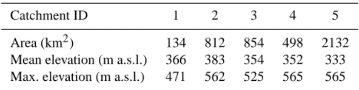
The catchment is centred at approximately 62.8◦N and 15.5◦E. The catchment area is 4400 km2 with a mean al-titude of 350 m a.s.l. (range: 20–540 m a.s.l.) and a mean annual precipitation of ∼700 mm. An area of 72×120 km (8640 km2), covering the Gim˚an catchment was selected as the study region and used when extracting data from the dif-ferent sources described below (Sects. 2.1–2.4). The catch-ment may be divided into five main subcatchcatch-ments (num-bered 1 to 5 in Fig. 1) and Table 1 shows some characteristics of the subcatchments. It can be seen that there is a gradient in mean elevation decreasing from west to east, but that the highest single elevations are in the eastern subcatchments.
Two radar sites cover the catchment, one ∼20 km north-west and one ∼100 km south-east of the catchment.
Precipitation data from five sources were analysed: NWP model, weather radar, precipitation gauges, and two versions of a mesoscale analysis system. All data were retrieved from the sources’ “operational versions”, i.e. the data sets are ac-tual products in the SMHI meteorological and hydrological forecasting systems, and thus reflect the current operational status in terms of data resolution and quality. For the present comparison, data from year 2002 were used. Although a longer time period would have been preferable, 2002 was selected as for this year consistent data from all sources be-low were readily available. Generally, 2002 was a slightly dry year in the region, with a total precipitation of ∼90% the long-term average. In particular late summer and autumn were drier than a normal year. Mean temperature in the re-gion in 2002 was ∼1.5◦C higher than the long-term average (SMHI, 2002).
2.1 NWP model (H22)
The numerical weather prediction model HIRLAM (High Resolution Limited Area Model) has been jointly developed by the weather services in Sweden, Norway, Finland, Den-mark, Iceland, Ireland, the Netherlands and Spain. The HIRLAM based precipitation estimates are dependent on the model characteristics, especially the physics parameterisa-tions. The model integration area of the SMHI HIRLAM version used in this study consists of 162×142 horizontal grid points at 22×22 km resolution and 31 vertical levels. Semi-Lagrangean time integration and a fourth order implicit horizontal diffusion scheme are used. The physics package included a first order local vertical diffusion scheme (Louis, 1979), a cloud and condensation scheme based on explicit forecasts of cloud water (Sundqvist et al., 1989) and a radia-tion scheme based on Savij¨arvi (1989). For the details of the various components of the HIRLAM forecasting system, see Und´en et al. (2002) and K¨all´en et al. (1996).
2.2 Mesoscale analysis (M22 and M11)
In the mesoscale analysis system at SMHI, MESAN, man-ual observations, automatic station data, satellite and radar imagery are combined by optimal interpolation. Represen-tativity and quality of each observation is taken into account in the interpolation, and the information content dependency on distance is modelled by so-called structure functions. Pre-cipitation analysis is performed using a variable first guess, which makes it possible to increase spatial resolution in data-sparse areas. The description of the error varies as a function of the prevailing weather situation (or precipitation amount). Generally, it is based on a statistically established relation between wind, orography and variations in friction and lati-tude, and approximately 50% of the observed climatological variance can be explained.
Table 1. Subcatchment characteristics.
Catchment ID 1 2 3 4 5
Area (km2) 134 812 854 498 2132 Mean elevation (m a.s.l.) 366 383 354 352 333 Max. elevation (m a.s.l.) 471 562 525 565 565
MESAN is run in two versions. One operational analysis based only on observations available in real-time, calculated in a 22×22 km grid (M22). One post-analysis (climate anal-ysis) including also quality controlled data from non-real-time climate stations and manual observations, calculated in a 11×11 km grid (M11). From the real-time analysis, in which HIRLAM output (Sect. 2.1) is used as the first guess in the optimal interpolation procedure, 12-h precipitation accu-mulations based on synoptical observations were used. From the climate analysis 24-h accumulations, and in this case the first guess consists of 12-h real-time analyses. Further infor-mation can be found in H¨aggmark et al. (1997, 2000).
2.3 Gauges (PTH)
PTHBV is a gridded precipitation (P) and temperature (T) database, intended to use as input in the HBV hydrologi-cal model. The grid is created by optimal interpolation from all available precipitation stations, corrected for catch losses using station specific factors with a seasonal variation (e.g. Alexandersson, 2003). In the interpolation scheme, frequen-cies of wind direction and wind speed are included in the description of the topographic influence. The horizontal res-olution of the PTHBV grid is 4×4 km and precipitation is available as 24-h accumulations. Further information about the interpolation procedure can be found in Johansson and Chen (2003, 2005).
2.4 Weather radar (RAD)
The accumulated precipitation radar product is based on re-flectivity products and synoptical observations. Gauge ad-justment is achieved by the method of Koistinen and Puhakka (1981) with a number of modifications (Michelson et al., 2000). Gauge accumulations are corrected using an imple-mentation of the Dynamic Correction Model presented by Førland et al. (1996), before they are used for the gauge adjustment (Michelson, 2004). If G denotes gauge obser-vation and R the simultaneous radar obserobser-vation, a general relationship between log(G/R) and range from the radar is derived using radar and gauge pairs from a 7-day moving time window. Depending on the number and quality of avail-able synoptical observations, this relationship can either be based on a parabolic regression or just the average log(G/R) value. The result is a field in which the quantitative accu-racy is largely determined by the gauge values and in which
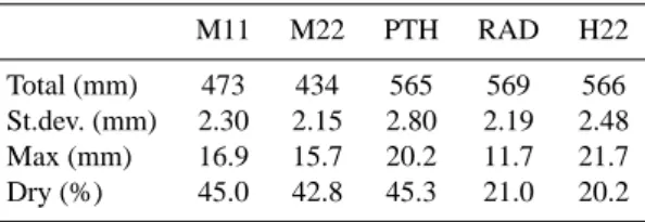
Table 2. Temporal statistics of daily mean areal precipitation in the
entire Gim˚an catchment during 2002.
M11 M22 PTH RAD H22 Total (mm) 473 434 565 569 566 St.dev. (mm) 2.30 2.15 2.80 2.19 2.48 Max (mm) 16.9 15.7 20.2 11.7 21.7 Dry (%) 45.0 42.8 45.3 21.0 20.2
the spatial distribution is determined by the radar data. The horizontal resolution of the radar products is 2×2 km, trans-formed from polar co-ordinates, and the temporal resolution is 3 h. Further information can be found in Michelson et al. (2000) and Koistinen and Michelson (2002).
2.5 Data preparation and general characteristics
Data from all sources were converted to the same tempo-ral resolution. The highest common tempotempo-ral resolution was 24 h, the original resolution of M11 and PTH. To achieve this for the HIRLAM output (H22), for each day the +6 h fore-casted accumulated total precipitation (i.e. the sum of con-vective and large-scale precipitation components) was sub-tracted from the +30 h forecast. For RAD eight 3-h compos-ites were summed and for M22 two 12-h accumulations were summed, to generate daily accumulations.
For each day, whole-catchment and subcatchment spatial averages were calculated for each of the sources, to be used in the subsequent runoff modelling. Error assessment was made mainly by studying seasonal subcatchment precipita-tion accumulaprecipita-tions and expressed as a relative error. Winter was defined as January-March, spring as April–June, sum-mer as July–September, and autumn as October–December.
Table 2 shows some descriptive statistics of the time series of daily whole-catchment averages. In terms of total precip-itation, the values from H22, PTH and RAD are all in the range 565–570 mm, whereas the values from the mesoscale analysis are significantly lower, especially the real-time M22. One obvious reason that M22 and M11 are lower than PTH is that the latter has been corrected for catch losses, as men-tioned in Sect. 2.3. This correction may explain the differ-ence between M11 and PTH. The fact that M22 is lower than M11 further indicates that rainfall amounts are underes-timated in the real-time synoptical observations, as the main difference between M22 and M11 is that in the latter data from climate stations are taken into account (Sect. 2.4).
Daily variability, as represented by the standard deviation, is clearly highest for PTH, followed by H22. The lower variability of M22 and M11 is possibly related to a gener-ally lower level of precipitation amounts, as indicated in the 2002 totals. The maximum value is generally rather close to 20 mm, the main exception being radar with only 11.7 mm.
This indicates an underestimation by RAD of large, areally extended rainfalls, which has also been found in e.g. Michel-son et al. (2000). Blocking effects is one possible cause, and this underestimation is likely also a reason for the low stan-dard deviation in the RAD data, found above. The percent-age of dry days, defined as having a mean areal precipitation less than 0.1 mm, is ∼45% for M22, M11 and PTH, but only
∼20% for H22 and RAD. In the case of H22, this indicates that the model generates small amounts of precipitation too often. This is a known tendency of NWP models. The low value for RAD similarly may indicate a frequent overesti-mation of light precipitation, but may also be related to the higher areal resolution of RAD and thus the possibility of detecting precipitation missed by gauges.
3 HBV model application
To investigate how differences and errors in the precipita-tion data propagate into the associated runoff, data from the different precipitation sources were used to drive the hydro-logical HBV model. In this section, the structure of the HBV model and its application in the Gim˚an catchment is described.
3.1 The HBV model
The HBV model (Bergstr¨om, 1976, 1992; Lindstr¨om et al., 1997) is a rainfall-runoff model which includes concep-tual numerical descriptions of hydrological processes at the catchment scale. It has been applied in a wide range of cli-mates and for scales ranging from lysimeter plots (Lindstr¨om and Rodhe, 1992) to the entire Baltic Sea drainage basin (Bergstr¨om and Carlsson, 1994; Graham, 1999). The model is used for flood forecasting in the Nordic countries and also, e.g., spillway design floods simulation (Bergstr¨om et al., 1992), water resources evaluation (Jutman, 1992; Brandt et al., 1994), and nutrient load estimates (Arheimer, 1998).
The general water balance in the HBV model can be de-scribed as
P − E − Q = d
dt[SP + SM + U Z + LZ + lakes] (1)
where P is precipitation, E is evapotranspiration, Q is runoff, SP is snow pack, SM is soil moisture, UZ is upper groundwater zone, LZ is lower groundwater zone, and lakes is the lake volume. Input data are observations of precipi-tation, air temperature and estimates of potential evapotran-spiration. The time step is usually one day, but it is possi-ble to use shorter time steps. The evaporation values used are normally monthly averages although it is possible to use daily values. Air temperature data are used for calculations of snow accumulation and melt and also, if required, to adjust potential evaporation.
The model consists of subroutines for meteorological in-terpolation, snow accumulation and melt, evapotranspiration
0 20 40 60 80 100 120 140 160 19821983 19841985 19861987 198819891990 19911992 19931994 199519961997 19981999 20002001 Year Q ( m 3/s ) Q OBS Q PTH
Fig. 2. Observed and simulated runoff in station Gimdalsbyn during the calibration period.
estimation, a soil moisture accounting procedure, routines for runoff generation and finally, a simple routing procedure be-tween subcatchments and in lakes. It is possible to run the model separately for several subcatchments and then add the contributions from all subcatchments. Calibration as well as forecasts can be made for each subcatchment. For basins of considerable elevation range a subdivision into elevation zones can also be made. This subdivision is made for the snow and soil moisture routines only. Each elevation zone can further be divided into different vegetation zones (e.g. forested and non-forested areas). Applying the model ne-cessitates calibration of a number of free parameters (around 10 in the present application). The model is equipped with an automatic calibration routine (e.g. Lindstr¨om, 1997), opti-mising one parameter at a time while keeping the others con-stant. The one-dimensional search is based on a modification of the Brent parabolic interpolation (Press et al., 1992).
3.2 Set-up, calibration and application
The HBV model has been set up for the Gim˚an catchment, divided into five subcatchments (Fig. 1), each specified in terms of altitude, vegetation and lake zones. Model cal-ibration was performed by the automatic calcal-ibration rou-tine described above, using 20 years of precipitation and temperature data (1982–2001) from the PTHBV database (Sect. 2.3). In the catchment, two discharge stations were available. Gimdalsbyn (G in Fig. 1), located at in the out-let of subcatchments 1–4, and Torpshammar (T in Fig. 1), at the outlet of the entire catchment. Therefore calibration was performed in two steps. In the first step parameter val-ues were obtained for subcatchments 1–4 by optimisation to station Gimdalsbyn. In the second step parameters for sub-catchment 5 were fixed by optimisation to station
Torpsham-mar. The result of the calibration for station Gimdalsbyn is shown in Fig. 2. The Nash-Sutcliffe model efficiency coeffi-cient R2(Nash and Sutcliffe, 1970) for the calibration period is 0.8965 and the relative volume error 0.004%; for Torp-shammar the values are 0.903 and 0.16%, respectively. It may be remarked that as the calibration was performed for PTHBV it may not be optimal for the other sources. How-ever, the limited available time periods with consistent data from the other sources makes accurate calibration impossi-ble. Further, having only one single set of model parameters facilitates interpretation of the results with focus on charac-teristics of the input data.
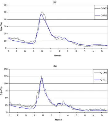
The calibrated HBV model was run for year 2002 us-ing the different types of precipitation input, and compared with the observed discharge in stations Gimdalsbyn and Torpshammar (Fig. 3). Concerning station Gimdalsbyn, the observed runoff exhibits a decreasing trend from Jan-uary (∼15 m3/s) until early April (<10 m3/s) , when spring flood starts. The spring flood reaches its peak in early May (∼50 m3/s), after which a rapid recession takes place until late June (∼15 m3/s), and in total the spring flood occurs al-most exactly within the spring as defined here. A comparison with Fig. 2 shows that the spring flood peak is rather low, be-low average. The second half of the year is characterised by a decreasing discharge which reaches its minimum in mid-October (<2 m3/s), to finally increase slowly to ∼4 m3/s at the end of the year. Concerning station Torpshammar, the more variable behaviour of the observed runoff, as compared with Gimdalsbyn, is due to the fact that this inflow has not been measured directly but estimated from measured values of lake outflow and change in lake volume. The latter is based on water level observations which are inherently un-certain because of natural fluctuations, and a small differ-ence in water level may have a great impact on lake volume
(a) 0 10 20 30 40 50 60 J F M A M J J A S O N D Month Q ( m 3/s ) Q OBS Q M11 (b) 0 25 50 75 100 125 150 J F M A M J J A S O N D Month Q ( m 3/s ) Q OBS Q M11
Fig. 3. Observed and simulated (M11) daily runoff in stations
Gim-dalsbyn (a) and Torpshammar (b) during 2002.
and in turn estimated discharge. To reduce the variability, 5-day running mean values of Q are shown in Fig. 3. The an-nual pattern is naturally similar to Gimdalsbyn, but the spring flood is somewhat more pronounced.
As initial model state at the start of the simulations on 1 January 2002, the final state from the calibration period (1982–2001) was used for all sources. To study the ef-fect of only precipitation input, in the runoff simulations the same temperature input was used for 2002 (from the PTHBV database; Sect. 2.3). The accuracy of the resulting runoff was interpreted in terms of visual agreement with observed runoff as well as the total and seasonal relative accumulated volume bias.
Besides the continuous 1-year runoff simulation experi-ment, a second experiment was performed, aimed at assess-ing how accurately the different sources were able to forecast the spring flood peak in late April and early May (Fig. 3). This forecasting experiment comprised the 2-week period 22 April to 5 May. For a certain day in this period, the cali-brated HBV model was first run from 1 January 2002 (using the same initial state as in the whole-year simulations above) to the previous day, using each of the different sources as in-put. Thus, at the time of the forecast, the different sources were associated with different HBV model states. Then the same actual 2-day forecast from the HIRLAM model was used as input, and a 2-day forecast run was performed. The HIRLAM forecast was produced by an earlier version of the model than described in Sect. 2.1, having a 44×44 km
reso-lution, and the forecast precipitation input was specified on subcatchment level. Overall forecast accuracy was specified in terms of the average relative discharge error over the 2-week period, for both 1 day and 2 days ahead forecasts.
4 Precipitation error assessment
In a strict sense, errors in precipitation estimates can not be calculated as there is no perfect observation system and thus no means of obtaining any “true” precipitation from which to estimate errors. Consequently a suitable baseline estimate must be selected, which albeit not perfect may represent the true rainfall and make possible an error assessment of other estimates. In the present study the mesoscale climate anal-ysis M11 is taken as the baseline source in the precipitation error assessment. M11 is a natural choice as it contains in-formation from the other sources, and as it has been adjusted using reliable climate station data. For each other source, error is expressed as a relative bias of accumulated precipita-tion, as compared with M11.
Concerning seasonal precipitation as represented in M11, in terms of amounts over the entire Gim˚an catchment most precipitation occurred in summer (∼150 mm), fol-lowed by spring (∼140 mm), winter (∼110 mm) and au-tumn (∼90 mm). Overall, seasonal precipitation is relatively evenly distributed over the catchment, with only ∼10 mm difference between the subcatchments with the highest and lowest amounts, respectively. Any obvious trend with mean altitude, implying an increase in precipitation towards the west (Table 1), cannot be found for the seasonal accumula-tions, even though during spring, summer and autumn the lowest amounts are indeed found in the eastern subcatch-ment 5. Winter precipitation, on the other hand, follows an opposite pattern, with a weak but systematic increase in pre-cipitation towards the east.
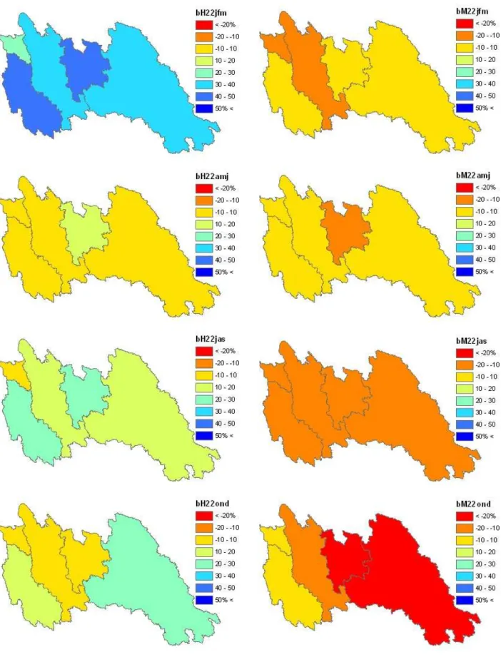
Figure 4 shows the seasonal subcatchment biases for all sources. Notice that the coloured scale is the same for all sources. Although it masks some intra-catchment variability, this has been done to illustrate the differences in bias levels between the sources.
Concerning source H22, a pronounced overestimation is found during winter, of a magnitude approaching 50% in subcatchments 2 and 4. An inspection of daily time series revealed that the total seasonal overestimation contains both small daily components, reflecting the tendency of the model to often generate small precipitation amounts, and large daily components, reflecting forecasted rainfall events that never materialised. During spring, the picture in Fig. 4 indicates a small bias, with most of the catchment being within 10% of M11. In reality, however, the case is one of compensating errors. In April, H22 virtually daily overestimated precipi-tation by 1–2 mm, whereas in June some fairly heavy rain-fall events were clearly underestimated by the model, by up to 8 mm. Summer and autumn are both characterized by an
Fig. 4. Relative accumulated precipitation bias (%) during winter (JFM), spring (AMJ), summer (JAS) and autumn (OND) 2002 for sources
Fig. 4. (Continued). Relative accumulated precipitation bias (%) during winter (JFM), spring (AMJ), summer (JAS) and autumn (OND)
overestimation of 10–30% over most of the catchment, with no clear spatial pattern. The overestimation in summer is largely owing to single events with lower rainfall amounts than forecasted.
Source M22 shows a good agreement with M11 in win-ter and spring, with only some minor underestimation in the central and western parts of the catchment. In summer, un-derestimation by 10–20% occurs over the entire catchment, resulting from small underestimations of many events, typ-ically by ∼2 mm. In autumn there is a spatial pattern with a good agreement with M11 in the west and a pronounced relative underestimation in the east. However, only ∼85 mm of precipitation occurred in subcatchment 5 during autumn, thus in absolute values the underestimation was less severe. The general underestimation by M22 may be related to un-derestimation in synoptical observations, as remarked above. In winter, source PTH exactly reproduces the spatial trend of M11, but consistently overestimates the precipitation by
∼25%. Time series inspection shows that the total overes-timation has both smaller and larger daily components. In the other seasons, the PTH bias ranges from being within 10% of M11 to overestimate by 30%, with a tendency to-wards more pronounced overestimation in the eastern part of the catchment, receiving the lowest amounts of precipitation. The general overestimation by PTH may be related to the correction for observation losses, as previously noted.
In spring and summer, source RAD generally reproduces the M11 levels and patterns to within 10%. The only no-table exception is a pronounced underestimation in ment 1 during summer. The M11 amount in this subcatch-ment and season is, however, substantially larger than in the other subcatchments. In autumn and winter, RAD overes-timates precipitation in the western part of the catchment. In winter, the average bias in subcatchments 1–4 is 20% but in autumn it is 66%, reaching 87% in subcatchment 1. From studying daily time series, the winter overestimation appears somewhat coincidental, as the season contains both daily over- and underestimations by RAD, of various magni-tude. In autumn, however, systematic daily overestimations are apparent. In particular, RAD observes a small amount of precipitation (∼1 mm) every day in autumn. A closer look at the original radar data revealed that the overestimations originate from single radar pixels with unrealistic precipita-tion amounts. This may be due temporary inaccuracies in the radar data, related to e.g. the existence of ground echoes or malfunctioning of the radar located north-west of the catch-ment.
5 Runoff error assessment
Similarly to precipitation, a runoff baseline estimate is re-quired for estimation of the associated errors or biases. One alternative is to use observed runoff as baseline. Defining errors as deviations from observations is intuitively sensible,
Table 3. Relative accumulated volume bias (%) in the runoff
simu-lations.
Station Period M22 PTH RAD H22 Gimdalsbyn JFM −1 2 3 4 AMJ −8 14 20 52 JAS −5 29 −15 1 OND −32 43 20 25 Torpshammar JFM 0 2 1 4 AMJ −4 15 10 57 JAS −11 36 −12 −12 OND −42 66 25 35
but this assumes a perfect model, i.e. that the model output is identical to the observations provided that the input is cor-rect. In reality, however, the runoff model is associated with an error (or uncertainty) and even for accurately specified input data the result will likely slightly differ from observa-tions (see Fig. 2). In light of this we use as runoff baseline the output from the HBV model when fed with the precipita-tion baseline estimate, i.e. M11. It can be argued that source PTH would provide a more appropriate runoff baseline esti-mate, as it was used in the HBV model calibration. However, for year 2002 source M11 reproduces observed runoff more accurately than any other source, including PTH. Because of this, and for consistency with the precipitation error assess-ment, we use M11 to define the runoff baseline estimate.
Figure 3 shows the agreement between observed runoff and runoff simulated using M11 data as input. For both runoff stations, the spring flood peak as well as the minor summer peak are overall well reproduced. The rising limb of the spring flood hydrograph is slightly delayed in the model and the peak slightly underestimated, but the recession is well captured. A notable deviation from the observations is found in winter, when the model systematically underesti-mates the runoff. As seen in Fig. 2, however, this type of winter underestimation is a rather common situation (e.g. the period 1983–1988) and may thus be viewed as a limitation in the model.
5.1 Continuous 1-year simulation
In Fig. 5, the result from the runoff simulations for 2002 is shown. Concerning station Gimdalsbyn (Fig. 5a), all sources are nearly identical during winter. In Table 3, seasonal rel-ative runoff volume biases are presented, and the minor dif-ferences in winter are manifested in biases of only a few per-cent. The reason for the similarity in simulated runoff is that the air temperature in winter is generally below 0◦C (mean January, February, March temperatures in 2002: −9.2◦C,
−4.7◦C, −3.7◦C), thus precipitation is stored in the snow pack, not immediately contributing to runoff.
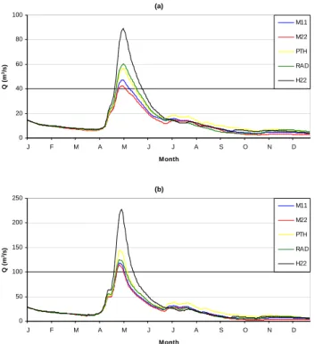
(a) 0 20 40 60 80 100 J F M A M J J A S O N D Month Q ( m 3/s ) M11 M22 PTH RAD H22 (b) 0 50 100 150 200 250 J F M A M J J A S O N D Month Q ( m 3/s ) M11 M22 PTH RAD H22
Fig. 5. Simulated runoff in stations Gimdalsbyn (a) and
Torpsham-mar (b) during 2002.
During the spring flood, however, substantial differences appear. Most striking is the flood peak overestimation by H22, with a peak discharge of nearly twice the baseline value of 47.4 m3/s. In terms of runoff volume, the overestima-tion is more than 50% (Table 3). An analysis of the simu-lation runs revealed that the main source of this discrepancy is the overestimated precipitation by H22 in winter (Fig. 4), mainly March, and spring (April). In March, the overesti-mated precipitation by H22 produced a snow depth approx-imately 20 mm (water equivalent) larger than M11. Snow melt occurred almost exactly within April (i.e. started 1 April and finished 30 April), but in reality this melt was not accom-panied by any significant precipitation, except for the last days in April and first days in May. H22, however, gener-ated a small amount of precipitation (∼1 mm) almost every day in April, as noted above in connection with Fig. 4. These small but frequent additions, in combination with some over-estimation of the heavy precipitation at the time of the spring flood peak in late April and early May, were the reasons for the overestimated spring flood.
Also RAD and PTH overestimates the spring flood, by 10– 15 m3/s in terms of peak discharge and 15–20% in terms of runoff volume. The overestimation by PTH is expected in light of the consistently overestimated winter precipitation in the entire catchment (Fig. 4). In the case of RAD, the over-estimation of winter precipitation was limited to subcatch-ments 1–3, therefore particularly affecting discharge in sta-tion Gimdalsbyn. Sources M22 slightly underestimates the
spring flood, in line with underestimated winter precipitation in subcatchments 1 and 3 (Fig. 4).
In summer a slight but consistent overestimation is found for PTH, partly extending into autumn, producing a volume bias of almost 30%. Looking at the spatial precipitation bi-ases (Fig. 4), summer precipitation is indeed overestimated by PTH, but even more so by H22, which did not cause any overestimated runoff. The reason for this discrepancy was found by inspection of daily precipitation error time series. The latter half of June was a wet period, and some overesti-mations by PTH in the last days of the month made discharge increase to an elevated level, which persisted all summer. Concerning H22, as mentioned above the summer overesti-mation of precipitation was largely associated with a few sin-gle events. Most of them occurred under relatively dry condi-tions, therefore they had little effect on runoff. An exception is in mid-September, when a week-long sequence of overes-timations by H22 is reflected in a slight increase in discharge (Fig. 5a). RAD underestimates the summer runoff volume by 15% (Table 3), which is related to the local but substantial underestimation of precipitation in subcatchment 1 (Fig. 4).
Also in autumn all sources agree rather well. M22 dis-charge is consistently at a slightly lower level, in line with the underestimated autumn precipitation (Fig. 4). The substan-tial overestimation of autumn precipitation by RAD, how-ever, has only a rather small impact on runoff. It is man-ifested in only a slight increase from mid-October to early November, after which the discharge level is rather stable (Fig. 5a). The reason for the limited impact on runoff can be found in the air temperature. Already in October, mean temperature was below 0◦C (−1.2◦C), but on single days the
temperature was up to 4◦C throughout the month.
There-fore in October the overestimated precipitation had some im-pact on runoff. In November and December, however, the temperature was consistently below 0◦C (mean temperatures
−6.9◦C and −10.6◦C, respectively), and the excess precip-itation in RAD was thus stored as snow. It may be noted that in relative terms the volume biases are large in autumn (Table 3), owing to the low discharge level.
Figure 5b shows the simulated runoff in station Torpsham-mar. Overall, the situation is very similar to that of station Gimdalsbyn, and thus is most of the above discussion valid also in this case. Also the relative volume biases are over-all similar to Gimdalsbyn, both in terms of magnitude and in terms of dependence on source and season (Table 3).
There are, however, some differences between the stations, which may be interpreted in terms of the spatial precipita-tion error distribuprecipita-tions. Concerning the spring flood, the overestimation by RAD is much less pronounced in Torp-shammar than in Gimdalsbyn, as winter precipitation was accurately estimated in the eastern part of the catchment (Fig. 4). The less pronounced underestimation by M22 can be explained similarly. In summer, the overestimation by PTH is somewhat more pronounced (36% volume bias, compared with 29% for Gimdalsbyn), which is in line with
32 0 4 8 12 16 20 24 28 1 2 3 4 5 6 7 8 9 10 11 12 13 Day P ( m m ) 0 20 40 60 80 100 120 140 Q ( m 3 /s ) P OBS (M11) P 1-day P 2-day Q OBS Q 1-day (M11) Q 2-day (M11)
Figure 6. Observed and forecasted (1- and 2-day; M11) catchment average precipitation and runoff in station Gimdalsbyn during 020423 (day 1) – 020505 (day 13).
Fig. 6. Observed and forecasted (1- and 2-day; M11) catchment
av-erage precipitation and runoff in station Gimdalsbyn during 020423 (day 1) – 020505 (day 13).
the more pronounced overestimation of precipitation in sub-catchment 5. In autumn, the more pronounced overestima-tion of precipitaoverestima-tion in subcatchment 5 by H22 and PTH and underestimation by M22 is reflected in larger volume biases than in station Gimdalsbyn (Table 3).
5.2 Spring flood peak forecasting
Figure 6 shows the HIRLAM 1-day (0–24 h) and 2-day (24– 48 h) precipitation forecasts during the 2-week forecasting period covering the spring flood peak. The values are catch-ment average values, and shown is also the observed average precipitation as represented by source M11. An overestima-tion of the precipitaoverestima-tion is apparent in the main rainy period (day 5–9), more pronounced in the 2-day than in the 1-day forecasts.
Also in the forecasting experiment, M11 was used as the baseline estimate, and Fig. 6 shows also the 1-day and 2-day M11 discharge forecasts for station Torpshammar, compared with the observed discharge. The 1-day forecast predicted very well the increase in discharge just before the peak, but failed to capture the sharp rise to the peak value and underes-timated the discharge by ∼10 m3/s in the latter part of the pe-riod. The fact that the forecast is rather smooth indicates that the contribution to the total discharge from forecasted precip-itation is small, compared with the contribution from snow melt. In fact the more pronounced overestimation of precip-itation in the 2-day forecasts made them perform somewhat better with respect to predicting the discharge peak. Still, in terms of root mean square error RMSE during the forecasting period, the 1-day forecast is slightly better, RMSE=10.7 m3/s compared with 10.9 m3/s for the 2-day forecast. The pic-ture is rather similar for station Gimdalsbyn but as expected from the lower discharge level the deviations are smaller, the RMSE values being 3.2 m3/s for the 1-day forecast and 3.7 m3/s for the 2-day forecast.
Table 4 presents the average relative discharge error dur-ing the forecastdur-ing period for the other sources, as compared
Table 4. Average relative discharge bias (%) in the forecasting
ex-periment.
Station Day M22 PTH RAD H22 Gimdalsbyn 1 −6 21 20 63
2 −7 22 20 65 Torpshammar 1 −4 30 8 79
2 −4 30 8 77
with M11. Overall it is obvious that the forecast performance is very much given by the discharge level at the start of the forecast period, as the rainfall amounts during the period are not large enough to have any substantial impact on the snow-melt dominated runoff. Therefore the numbers in Table 4 largely reflect the situation displayed in Fig. 5. In Gim-dalsbyn, H22 overestimates discharge by more than 60%, PTH and RAD by ∼20%, and M22 slightly underestimates it. The main differences in station Torpshammar is a more pronounced overestimation by H22 and a less pronounced overestimation by RAD. In total, the main outcome from the forecasting experiment is a numerical quantification of the different sources’ performance with respect to reproducing the spring flood peak.
6 Summary and conclusions
The present study aimed at investigating the propagation of spatio-temporal errors in precipitation estimates to runoff er-rors in the output from the conceptual hydrological HBV model. The perspective was operational, involving both pre-cipitation products and model set-up as used operationally in the SMHI forecasting system. The study region was the Gim˚an catchment in central Sweden, which has expe-rienced flooding problems in recent years, and the study period year 2002. Five precipitation sources were consid-ered: NWP model (H22), weather radar (RAD), precipita-tion gauges (PTH), and two versions of a mesoscale analy-sis system (M11, M22). To define the baseline estimates of precipitation and runoff, used to define errors, the mesoscale climate analysis M11 was used.
The precipitation error assessment indicated a systematic overestimation of precipitation by H22, in particular during winter and early spring, reflecting a too frequent generation of light precipitation by the model. M22 generally underes-timated precipitation, possibly related to underestimation in synoptical observations. Probably because of a correction for observation losses, PTH overestimated precipitation. RAD was characterized by a pronounced local overestimation dur-ing autumn, in the western part of the catchment, indicatdur-ing inaccuracies in the performance of a particular radar. The seasonal subcatchment relative accumulated volume biases
were generally within ±20%, but overestimations up to 30– 50% were not uncommon, in some case approaching 100%.
The data from the different sources were used to drive the HBV model, set up and calibrated for two stations in Gim˚an, both for continuous simulation during 2002 and for forecasting of the spring flood peak. In winter the differ-ence in runoff between the sources was negligible, as cipitation was stored as snow and base-flow conditions pre-vailed. In spring substantial biases appeared, most notably for H22 which overestimated the accumulated runoff volume by ∼50% and peak discharge by almost 100%, at both sta-tions. This was a combined effect of overestimations of both snow depth and precipitation during the rising limb of the spring flood hydrograph. PTH overestimated spring runoff volumes by ∼15% at both stations, in line with overesti-mated winter precipitation. For RAD and M22 the result fered somewhat between the stations, reflecting spatial dif-ferences in the precipitation biases. In summer and autumn runoff from all sources agreed rather well, even if relative biases were comparably large owing to low discharge levels. The pronounced overestimation of precipitation by RAD in autumn did not have any strong impact on runoff as it was mainly stored as snow. The forecasting experiment provided a clearer picture of model performance during the spring flood, with relative average discharge errors of up to 80% for H22 and within ±30% for the other sources.
We conclude that the errors or biases in precipitation from different sources exhibit a complex space-time variability, at scales relevant in rural hydrology. The largest biases were found in data from sources H22 and RAD, which was expected as they represent model forecasted and remotely sensed precipitation, respectively. Still, for most seasons and subcatchments, precipitation volumes from these sources were within ±20% of the baseline estimate, which is encour-aging. The runoff modelling experiments clearly demon-strated another feature of the precipitation biasess, namely that they may become either magnified or reduced when ap-plied for hydrological purposes, depending on both temporal and spatial variations in the catchment. Temporal variations may be related to e.g. the dynamics of air temperature and soil moisture, which both influence to which degree precip-itation is stored or directly transformed into runoff. Spatial variations may concern e.g. altitude or distance to catchment outlet. Thus, for optimal use in hydrological forecasting sys-tems, it is desirable that the uncertainty in precipitation esti-mates is specified as a function of both time and space.
Finally we wish to emphasise that this is a case study, observations made and conclusions drawn are strictly valid only for the specific time period and region under investiga-tion. Concerning time, one year is clearly not enough for a proper long-term assessment of systematic differences be-tween sources. On the other hand, as both models and analy-sis systems are under constant development, it may be prac-tically impossible to obtain consistent historical output for all sources during longer time periods. Concerning area, the
size of the study region is rather small, especially in rela-tion to the 22×22 km resolurela-tion of H22 and MA22. Further, the temporal and areal representativity of a certain time pe-riod and region is always to some extent unknown, but it is clear that in the present case neither time period nor region represents any extreme conditions. Nevertheless, further in-vestigations are required to judge to which degree the results obtained in the present study can be generalised.
Acknowledgements. The present investigation was performed within the EU-project CARPE DIEM (contract no. EVG1-CT-2001-0045). I thank two anonymous reviewers for their constructive criticism and B. Johansson and G. Grahn for helpful support and fruitful discussions.
Edited by: M. Bruen Reviewed by: two referees
References
Alexandersson, H.: Correction of precipitation with a simple clima-tological approach (in Swedish), SMHI Reports Meteorology, nr. 111, 2003.
Arheimer, B.: Riverine Nitrogen – analysis and modelling under Nordic conditions, Kanaltryckeriet, Motala, 1998.
Bergstr¨om, S.: Development and application of a conceptual runoff model for Scandinavian catchments, SMHI Reports Hydrology and Oceanography, nr. 7, 1976.
Bergstr¨om, S.: The HBV model – its structure and applications, SMHI Reports Hydrology, nr. 4, 1992.
Bergstr¨om, S. and Carlsson, B.: River runoff to the Baltic Sea: 1950–1990, Ambio, 23, 280–287, 1994.
Bergstr¨om, S., Harlin, J., and Lindstr¨om, G.: Spillway design floods in Sweden. I: New guidelines, Hydrol. Sci. J., 37, 505–519, 1992. Brandt, M., Jutman, T., and Alexandersson, H.: The water bal-ance of Sweden, Annual mean values 1961–1990 of precipita-tion, evaporation and runoff (in Swedish), SMHI Reports Hy-drology, nr. 49, 1994.
Carpenter, T. M. and Georgakakos, K. P.: Impacts of parametric and radar rainfall uncertainty on the ensemble streamflow simu-lations of a distributed hydrologic model, J. Hydrol., 298, 202– 221, 2004.
Chaubey, I., Haan, C. T., Grunwald, S., and Salisbury, J. M.: Uncer-tainty in the model parameters due to spatial variability of rain-fall, J. Hydrol., 220, 48–61, 1999.
Førland, E. J., Allerup, P., Dahlstr¨om, B., Elomaa, E., Jonsson, J., Madsen, H., Per¨al¨a, J., Rissanan, P., Vedin, H., and Vejen, F.: Manual for operational correction of nordic precipitation data, DNMI Report nr. 24/96, Norwegian Meteorological Institute, Norway, 1996.
Graham, P.: Modelling runoff to the Baltic basin. Ambio, 28, 328– 334, 1999.
H¨aggmark, L., Ivarsson, K.-I., and Olofsson, P.-O.: MESAN – Mesoscale Analysis (in Swedish), SMHI Reports Meteorology and Climatology, nr. 75, 1997.
H¨aggmark, L., Ivarsson, K.-I., Gollvik, S., and Olofsson, P.-O.: Mesan, an operational mesoscale analysis system, Tellus, 52A, 2–20, 2000.
Hossain, F., Anagnostou, E. N., Dinku, T., and Borga, M.: Hydro-logical model sensitivity to parameter and radar rainfall estima-tion uncertainty, Hydrol. Processes, 18, 3277–3291, 2004. Johansson, B. and Chen, D.: The influence of wind and topography
on precipitation distribution in Sweden: Statistical analysis and modelling, Int. J. Climatol., 23, 1523–1535, 2003.
Johansson, B. and Chen, D.: Estimation of areal precipitation for runoff modelling using wind data: a case study in Sweden, Clim. Res., 29, 53–61, 2005.
Jutman, T.:. Production of a new runoff map of Sweden. Proceed-ings of Nordic Hydrological Conference, 4–6 August, Alta, Nor-way, NHP report, nr. 30, 643–651, 1992.
K¨all´en, E.: HIRLAM Documentation Manual, Available from SMHI, 60176 Norrk¨oping, Sweden, 1996.
Koistinen, J. and Michelson, D. B.: BALTEX weather radar-based products and their accuracies, Boreal Env. Res., 7, 253–163, 2002.
Koistinen, J. and Puhakka, T.: An improved spatial gauge-radar ad-justment technique, Preprints 20th AMS Conf. on Radar Met., 30 November–3 December, Boston, MA., 179–186, 1981. Kyriakidis, P. C., Miller, N. L., and Kim, J.: Uncertainty
propaga-tion of regional climate model precipitapropaga-tion forecasts to hydro-logic impact assessment, J. Hydrometeorol., 2, 140–160, 2001. Lindstr¨om, G.: A simple automatic calibration routine for the HBV
Model, Nordic Hydrol., 28, 153–168, 1997.
Lindstr¨om, G. and Rodhe, A.: Transit times of water in soil lysime-ters from modelling of oxygen-18, Water, Air and Soil Pollution, 65, 83–100, 1992.
Lindstr¨om, G., Johansson, B., Persson, M., Gardelin, M., and Bergstr¨om, S.: Development and test of the distributed HBV-96 hydrological model, J. Hydrol., 201, 272–288, 1997.
Louis, J. F.: A parametric model of vertical eddy fluxes in the atmo-sphere, Bound.-Layer Meteorol., 17, 187–202, 1979.
Maskey, S., Guinot, V., and Price, R. K.: Treatment of precipitation uncertainity in rainfall-runoff modelling: a fuzzy set approach, Adv. Water Resour., 27, 889–898, 2004.
Michelson, D. B.: Systematic correction of precipitation gauge ob-servations using analyzed meteorological variables, J. Hydrol., 290, 161–170, 2004.
Michelson, D. B., Andersson, T., Koistinen, J., Collier, C. G., Riedl, J., Szturc, J., Gjertsen, U., Nielsen, A., and Overgaard, S.: BALTEX Radar Data Centre products and their methodologies, SMHI Reports Meteorology and Climatology, nr. 90, 2000. Nandakumar, N. and Mein, R. G.: Uncertainty in rainfall-runoff
model simulations and the implications for predicting the hydro-logic effects of land-use change, J. Hydrol., 192, 211–232, 1997. Nash, J. E. and Sutcliffe, J. V.: River flow forecasting through con-ceptual models. Part I: A discussion of principles, J. Hydrol., 10, 282–290.
Nijssen, B. and Lettenmaier, D. P.: Effect of precipitation sam-pling error on simulated hydrological fluxes and states: Antic-ipating the Global Precipitation Measurement satellites, J. Geo-phys. Res., 109, D02103, doi:10.1029/2003JD003497, 2004. Press, W. H., Teukolsky, S. A., Vetterling, W. T., and Flannery, B.
P.: Numerical Recipes in FORTRAN, The Art of Scientific Com-puting, Second Edition, Cambridge Univ. Press, 1992.
Savij¨arvi, H.: Fast radiation parameterization schemes for mesoscale and short-range forecast models, J. Appl. Meteorol., 29, 437–447, 1989.
Sharif, H. O., Odgen, F. L., Krajewski, W. F., and Xue, M.: Numeri-cal simulations of radar rainfall error propagation, Water Resour. Res., 38, 8, doi:10.1029/2001WR000525, 2002.
Sundqvist, H., Berge, E., and Kristjansson, J. E.: Condensation and cloud parameterization studies with a mesoscale numeri-cal weather prediction model, Mon. Wea. Rev., 117, 1641–1657, 1989.
Swedish Meteorological and Hydrological Institute (SMHI): Weather and Water – the Weather Year 2002 (in Swedish), V¨ader och Vatten, nr. 13, SMHI, Norrk¨oping, Sweden, 2002.
Todini, E.: A Bayesian technique for conditioning radar precipita-tion estimates to rain-gauge measurements, Hydrol. Earth Syst. Sci., 5, 187–199, 2001,
http://www.hydrol-earth-syst-sci.net/5/187/2001/.
Und´en, P., Rontu, L., J¨arvinen, H., Lynch, P., Calvo, J., Cats, G., Cuxart, J., Eerola, K., Fortelius, C., Antonio Garcia-Moya, J., Jones, C., Lenderlink, G., McDonald, A., McGrath, R., Navas-cues, B., Woetman Nielsen, N., Ødegaard, V., Rodriguez, E., Rummukainen, M., R˜o˜om, R., Sattler, K., Hansen Sass, B., Savij¨arvi, H., Wichers Schreur, B., Sigg, R., The, H., and Tijm, A.: HIRLAM-5 Scientific Documentation, available from SMHI, 60176 Norrk¨oping, Sweden, 2002.