Design of a single element 3D ultrasound scanner

(1)

Design of a Single Element 3D Ultrasound Scanner

by

Xiang Zhang

B.S. University of Maryland (2013)

Submitted to the Department of Mechanical Engineering

in partial fulfillment of the requirements for the degree of

Master of Science in Mechanical Engineering

at the

MASSACHUSETTS INSTITUTE OF TECHNOLOGY

June 2015

c

○ Massachusetts Institute of Technology 2015. All rights reserved.

Author . . . .

Department of Mechanical Engineering

May 8, 2015

Certified by . . . .

Brian W. Anthony

Principal Research Scientist, Department of Mechanical Engineering

Thesis Supervisor

Accepted by . . . .

David E. Hardt

Graduate Officer, Department of Mechanical Engineering

(2)

(3)

Design of a Single Element 3D Ultrasound Scanner

by

Xiang Zhang

Submitted to the Department of Mechanical Engineering on May 8, 2015, in partial fulfillment of the

requirements for the degree of

Master of Science in Mechanical Engineering

Abstract

Over the past decade, substantial effort has been directed toward developing ultra-sonic systems for medical imaging. With advances in computational power, previously theorized scanning methods such as ultrasound tomography can now be realized. This thesis presents the design, error analysis, and initial image reconstructions from a sin-gle element 3D ultrasound tomography system. The system enables volumetric pulse echo or transmission imaging of distal limbs, for applications including: improving prosthetic fittings, monitoring bone density, and characterizing muscle health. The system is designed as a flexible mechanical platform for iterative development of algorithms targeting imaging of soft tissue with bone. The mechanical system in-dependently controls movement of two single element ultrasound transducers in a cylindrical water tank. Each transducer can independently circle about the center of the tank as well as move vertically in depth. High resolution positioning feedback (∼1𝜇m) and control enables flexible positioning of the transmitter and the receiver around the cylindrical tank; exchangeable transducers enable algorithm testing with varying transducer frequencies and beam geometries. High speed data acquisition (DAQ) through a dedicated National Instrument PXI setup streams digitized data directly to the host PC. System positioning error has been quantified and is within limits for the desired imaging modality. Imaging of various objects including: cal-ibration objects, phantoms, bone, animal tissue, and human forearm are presented accordingly.

Thesis Supervisor: Brian W. Anthony

(4)

(5)

Acknowledgments

I would like to thank my advisor Brian Anthony for the continued guidance and sup-port during this project. Brian’s expansive set of knowledge helped guide me through the previously unfamiliar territories in this project. In addition, Brian always helped support the project needs in both hardware and software, but more importantly adding the right personnel to move the project forward.

I would also like to thank Jon Fincke, our resident acoustics expert. His under-standing of acoustic imaging has helped push the project forward in both algorithm development and how to improve the mechanical design. His acoustic data processing skills and Matlab expertise has helped crunch much of the data I have produced.

I’d also like to thank Stephen Racca and the "Bench to Bucks" team for their concept generation and additional prototyping after completion of the class.

(6)

(7)

List of Figures

1-1 Comparison of UST images to MRI images . . . 18

2-1 Ring array systems . . . 24

2-2 Conical transducer array . . . 25

2-3 Array probe with reflector [8] . . . 26

2-4 Reflector tomography . . . 27

2-5 36 angle reflector tomography at multiple heights . . . 27

3-1 Cylindrical Scanning Layout . . . 30

3-2 Cylindrical Scanning Layout . . . 30

3-3 Dual ring bearing . . . 34

3-4 Tracked design . . . 35

3-5 Dual arm design . . . 35

3-6 Through tank design . . . 36

3-7 Nested tank design . . . 36

4-1 Scanner 3D coordinate system. . . 40

4-2 Bearings choices for angular rotation . . . 41

4-3 Cross section of transducer bracket . . . 43

4-4 High resolution encoding setup and drive pinion . . . 44

4-5 LabView angular control VI for a single motor . . . 45

4-6 LabView stepper control VI . . . 47

4-7 Full scanning system with calibration plate . . . 48

(12)

5-2 Custom FPGA personality for high speed triggering . . . 53

5-3 DAQ schematic and synchronization . . . 53

6-1 0.5in nylon 6-6 rod centered in the tank on the calibration plate. . . . 56

6-2 DAQ Stability. . . 58

6-3 Mechanical Positioning Error. . . 59

6-4 Simulated transducer beam pattern. . . 60

6-5 Measured transducer beam pattern. . . 61

7-1 B-mode images of centered cylindrically symmetric objects . . . 63

7-2 Object distortions in Cartesian and Polar coordinates . . . 64

7-3 Angular Insensitivity of a omni-directional source . . . 65

7-4 Defined transducer (R) and point scatterer (P) coordinates for Eq. 7.1 66 7-5 Profile of a point scatterer at (0,60mm) viewed in pulse-echo by an omni-directional source/receiver moving in a circular aperture . . . . 66

7-6 Image correction algorithms flow chart . . . 68

7-7 Correct images after migration . . . 69

7-8 Vertical steel rod scans . . . 70

7-9 Corrected vertical steel rod scans . . . 70

7-10 Axial scan of steel rod with steel collars. . . 71

7-11 Axial scan of steel collars on a steel rod at various separations . . . . 72

7-12 Top and bottom view of scanned lamb long bone . . . 73

7-13 Lamb long bone at viewed at various angles . . . 74

7-14 Exemplary scan angular and axial scan planes . . . 74

7-15 Angular scan of a lamb long bone . . . 75

7-16 Axial scan of a lamb long bone . . . 75

7-17 Forearm angular scans . . . 76

8-1 Planar scanning of a lamb bone at various heights . . . 80

8-2 Axial scanning of a lamb bone at various fixed angular positions . . . 81

(13)

9-2 Tomographic imaging of a pig limb section . . . 85 9-3 Transmission B-mode images . . . 86 9-4 Spectrogram of received signals . . . 86

(14)

(15)

List of Tables

2.1 Comparison of system architectures . . . 28

3.1 Attenuation coefficient of various biological tissues [14] . . . 31

3.2 Concept Selection Pugh Chart . . . 37

(16)

(17)

Chapter 1 Introduction

Ultrasound imaging has been used widely in the clinical setting for several decades. It is inherently safe and cost-effective, compared to other major imaging modalities such as X-ray, computed tomography (CT), and magnetic resonance imaging (MRI). Comparing the number of ultrasound procedures done globally in 2011 versus the number done in 2000, there has been more than an order of magnitude increase in quantity (250M → 2800M) [26]. Whereas, the number of MRI and CT scans only doubled (35M → 80M and 75M → 160M respectively). However, the number of dig-ital X-ray procedures in 2011 (3300M) did surpass ultrasound [26]. This is likely due better penetration of X-rays through the body when compared to ultrasound. How-ever, X-rays procedures expose patients to ionizing radiation and X-ray machines are generally costly and non-portable. With the increase in transistor density following Moore’s Law and the miniaturization of electronic devices, ultrasound systems have evolved from bulky work stations to laptop sized portables. Additional ultrasound imaging modes such as doppler, 3D, and elastography, have also been enabled.

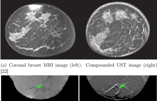
The image quality of ultrasound is typically lower than other modalities. Recent research into ultrasound tomography (UST) has mitigated this statement. The UST principle has been known since the 1970s [24], but only recently has computational power become sufficient to reconstruct images on clinically relevant time scales. UST systems incorporating ultrasound transmission and reflection data of the breast have produced images with qualities comparable to those of MRI [22] [11]. As seen in

(18)

Fig. 1-1a and Fig. 1-1b, UST images are almost indistinguishable from MRI images. Quantitative speed of sound and attenuation mapping of the breast with UST can also diagnose and localize tumors via differences in tissue density [21].

(a) Coronal breast MRI image (left). Compounded UST image (right) [22]

(b) Sagittal breast MRI image with image registration (left). Com-pounded UST image (right) [11]

Figure 1-1: Comparison of UST images to MRI images

Inspired from the UST results, we aim to utilize the UST technique for volumet-ric limb imaging. Unlike soft tissue imaging of the breast, limb imaging gives rise to complex propagation modes, mode conversion, and multiple paths due to the pres-ence of bone. At typical medical ultrasound frequencies (1-5MHz ), bones typically cause shadowing within the image. However, transmission of ultrasound is possible at lower frequencies (0.5-1MHz ) and have been used classify patients with and without osteoporosis [13]. To develop a UST system for volumetric limb imaging, innovations in both hardware and software are necessary. Novel scanning systems are needed, including transducers, mechanical positioning structures and actuators, and data ac-quisition setups. The scanning system must be capable of recording both reflected and transmitted waves inside the appropriate scan volume. New algorithms

(19)

account-ing for the complex propagation of sound waves in bone are necessary to accurately reconstruct tomographic data. The developed hardware should be sufficiently flex-ible to support rapid and iterative development of various complex algorithms and support use of various transducers.

1.1 Clinical Motivation

Using ultrasound to image bone and the surrounding tissue results in strong refraction, attenuation, and scattering of the transmitted acoustic waves. Typical assumptions made in soft tissue imaging do not hold with the presence of bone. In this regard, scans of soft tissue with bone presents an interesting set of new imaging challenges and applications [14]. Accurate quantitative characterization of bone and surrounding soft tissues has wide potential in BLANK applications. We consider several motivating clinical needs: (1) improve prosthetic fittings by integrating internal tissue and bone structural information into the socket design process [4], (2) monitor bone density deterioration for osteoporosis progression and diagnosis [13], and (3) better quantify neuromuscular disease progression such as Duchenne’s muscular dystrophy [6].

1.1.1 Prosthetic Fitting

The current plaster casting method for prosthetic fitting is a largely subjective process [16]. Typical fittings require several iteration to achieve a desirable fit. Improper fittings at the limb-socket interface can cause neuromas, inflammation, soft tissue calcifications, and pressure sores [16]. Any of these pain inducing pathologies can force the wearer into a wheelchair or crutches, reducing their mobility and quality of life. The prosthetics fitting challenge hinges on the ability to record skin and bone surfaces of adequately high-resolution. A 3D ultrasound system capable of accurately segmenting the skin surface and the bone surface, while being integrated into a prosthetic CAD modeling system will substantially improve the socket design process [27].

(20)

1.1.2 Bone Mineral Density Monitoring

Osteoporosis (a condition under which the bone mineral density (BMD) is substan-tially reduced) is a condition affecting a significant part (>50% in the US) of the population aged 50 and above [19]. Osteoporosis greatly increases the risk of frac-tures, which can be particularly debilitating at the older age. Early diagnosis, quan-titative measurement, and monitoring are important to manage the progression of the condition, but also to assess the efficacy of new treatments. Currently, X-ray is the predominant imaging modality for such diagnosis and monitoring. However, it is estimated that one must lose ∼30% of BMD to be noted on X-rays [19]. A more sen-sitive testing modality could provide earlier osteoporosis diagnosis and improve BMD measurement accuracy. The clinical potential of ultrasound to study bone fractures was first explored for monitoring of fracture healing [12]. Variation in the transmis-sion of ultrasound through the heel can be used to classify patients with and without osteoporosis [13]. Volumetric ultrasound imaging through a distal limb could be used to volumetrically map the speed of sound and attenuation inside the bone, providing a richer set of measurements of the bone mineral density.

1.1.3 Muscle Deterioration Monitoring

Characterized by progressive disability leading to death, Duchenne muscular dystro-phy (DMD) remains one of the most common and devastating neuromuscular disor-ders of childhood [3]. It is caused by a genetic mutation which generates a complex sequence of events in muscle cells which eventually undergo fibrosis and are replaced by adipose and connective tissue. Average survival of DMD patients is to the age of 25, although in some cases patients have survived into their forties. Although a vari-ety of promising new treatment strategies are in development, outcome measures for clinical trials remain limited for the most part to a set of functional measures, such as the six-minute walk test [6]. While clearly useful, such measures are impacted by unrelated factors, such as mood and effort, and have limited repeatability. To address this and other limitations, magnetic resonance imaging (MRI) is now being

(21)

investigated as a surrogate measure. However, more easily applicable, cost-effective, office-based surrogate measures that provide high repeatability and sensitivity while still correlating strongly to disease status would find wider use in Phase II and possi-bly in Phase III clinical trials in DMD. A 3D ultrasound system capable of providing quantitative measurements of the muscle deterioration can serve as a convenient, non-invasive, clinically meaningful method to track DMD disease progression that surpasses the functional measures currently in use.

1.2 Thesis Scope

This thesis describes the design of a 3D ultrasound imaging system capable of both reflective and transmission imaging of a limb. In Chapter 2 and 3, existing UST sys-tems are first described and system requirements for volumetric tomographic imaging are extracted with reference to the defined clinical motivations. Detailed mechan-ical and electrmechan-ical design and construction of the system is presented in Chapter 4 and 5, followed by system characterization in Chapter 6. Initial echo imaging and tomography scans on the completed system is presented in Chapter 7-9.

(22)

(23)

Chapter 2 Ultrasound Tomography

With the increase of computational power in the past decade, ultrasound tomography (UST) is emerging as a promising new imaging modality for imaging of soft tissues. Recent systems targeting in-vivo breast imaging have produced clinically relevant images with quality and resolution comparable to those of MRI [5], [11]. However, an UST system for in-vivo imaging and quantitative characterization of soft tissue surrounding bone has not yet been developed. For this thesis, we aim to design a system that supports iterative development and testing of algorithms for ultrasound imaging of soft tissue with bone motivated by a few target clinical applications.

2.1 Soft Tissue Ultrasound Tomography Systems

The kinematics of current UST enabled systems vary greatly to accommodate the respective transducer architectures. Transducer architectures include: ring arrays, conical arrays, array probes, and single elements. Advantages and disadvantages for each architecture will be evaluated in the following sections, with reference to designing a rapid algorithm development system to target the clinical motivations listed in Chapter 1.

(24)

2.1.1 Ring Arrays

Ring transducer systems typically consists of a rigid ring transducer (256-2048 ele-ments) scanning in one axis along the target, reconstructing 2D slices of the object. Such systems were the first to provide clinically relevant data and obtain FDA ap-proval [5]. The first Computed Ultrasound Risk Evaluation prototype (CURE) devel-oped by Duric et al. used a 20cm diameter ring transducer consisting of 256 elements [5]. The system produced compounded breast ultrasound images of quality rivaling those of MRI [22]. A denser ring transducer (15cm 2048 elements) system was de-signed by Waag and Fedewa, but has not been used for clinical imaging [28]. The two systems shown in Fig, 2-1 below, enable reflective imaging with attenuation and sound speed mapping within the circular aperture. Due to the high number of trans-ducers, complex data acquisition (DAQ) hardware is necessary for parallel sampling of the numerous receive channels. Custom sampling and multiplexing hardware were developed for each scan system. Custom ring transducers are costly when compared to commercial hand held probes and are not easily exchangeable.

(a) CURE system by Duric et al [5]. (b) Ring array system by Waag and Fedewa [28].

Figure 2-1: Ring array systems

Ring transducers provide great image quality within the horizontal (in-plane) circular aperture (Fig. 1-1a), but the slice thickness (out-of-plane) is limited (12mm in the CURE system) [5]. The difference in in-plane and out-of-plane resolution creates an anisotropic voxel sizes in the volumetric reconstructions, limiting imaging

(25)

to coronal breast slices.

2.1.2 Conical Arrays

To correct the anisotropic resolution in ring transducer systems and enable non-sliced 3D tomography, a conical array system for breast imaging was developed by Hopp et al. The conical system consist of 628 transmitters and 1413 receivers forming a 26cm diameter 18cm height semi-ellipsoidal aperture around the breast. Producing up to 80GB of data per scan on an FPGA-based sampling system, reflection, attenuation, and sound speed mapping is possible in spherical 3D coordinates [11]. The conical array is shown in Fig. 2-2.

Figure 2-2: Conical transducer array

With out of plane receivers, the conical array system can produce isotropic voxels in volumetric imaging. This enables extraction of transverse and sagittal volume slices shown in Fig. 1-1b, which is not possible in sliced based systems.

Relative to ring transducers, conical arrays have more transducer elements. DAQ and processing systems for the conical array is as complex, if not more complex, than the systems for ring transducers, but recent implementation of FPGAs and GPU pro-cessing has helped improve data throughput and propro-cessing [2]. The manufacturing complexity and cost of a conical array does not enable geometric flexibility in the system. Despite the transducer density, both the ring and conical arrays are still undersampling the slice or volume, respectively [23].

(26)

2.1.3 Array Probe Scanner

Mechanical sweeping with an array probe provides added system flexibility at the cost of scanning speed. Mechanical scanning with commercial array probes has been used for boundary detection for improving prosthetic fittings [4]. Commercially available probes do not support tomographic scanning and require an additional receiver to sample transmission data. Hansen et al. bypassed this limitation by adding an acoustic mirror opposing the transmitter [8]. Shown in Fig. 2-3, the stainless steel acoustic mirror reflects the incident wave back to the transmitter, providing through transmission data without a receiver. Ray tracing based on the arrival time of the reflected wave enables sound speed and attenuation mapping within the image slice.

(a) (b)

Figure 2-3: Array probe with reflector [8]

Images (Fig. 2-4) are produced on the reflector system with as few as 3 insonifying angles (60∘, 140∘, 260∘). Higher quality images are produced with 36 insonifying angles at 10∘ increments at multiple heights (Fig. 2-5) [10]

The reflector tomography system suffers from the slice thickness limitation as with the ring transducer system. The inability to capture off angle reflections limits imaging to coronal breast slices. From the cost perspective, commercial ultrasound probe and system costs ∼$10,000 per probe and ∼$100,000 to ∼$250,000 per sys-tem. Though likely cheaper than the ring array and conical array systems (pricing unavailable) $10,000 to exchange a transducer for testing and development is still non-trivial.

(27)

Figure 2-4: Reflector tomography

Figure 2-5: 36 angle reflector tomography at multiple heights

2.2 Single Element Scanning

For rapid iterative algorithm development, a system is required that is flexible and simple. The system should provide flexible transducer configurations (frequency/beam geometry) in conjunction with accurate transducer positioning. With high production cost and system complexity, ring and conical arrays are unsuitable for flexible itera-tive development. Array probes do provide more flexibility but cost is still high per probe (∼$10,000) and data acquisition flexibility is dependent on the corresponding probe imager manufacturer.

Single element scanning with one transmit and one receive channel is well suited at the developmental stages. Exchangeable transducers and single channel data acqui-sition significantly reduces cost and system complexity, while maintaining flexibility and low-level control of the system.

However, the flexibility and simplicity of a single element scanning system sacri-fices the scanning speed. The transmit and receive transducers must be mechanically

(28)

placed at each sampling locations around the aperture to complete a scan. Mechan-ical positioning will always be slower than electronic switching but does allow for custom sampling resolution around the aperture. In reference to prosthetic fitting, as dicussed by Mak et al. [16], patient movement during a scan heavily affects the re-sulting image. Motion compensation or tracking may be necessary at lower scanning speeds to correct for patient motion.

2.3 Summary

An overview of ultrasound tomography was first given. Relevant tomographic systems using ring arrays, conical arrays, array probes, and single elements were discussed. Capabilities and limitations of each transducer architecture were presented and eval-uated with reference to designing a developmental system for bone imaging. In con-clusion, single element scanning offered the best flexibility, cost effectiveness, and simplicity for a developmental system. A summarized Pugh chart comparison with the ring transducer system as a reference is presented. in Table [TABLE]. Design, construction, characterization, and imaging with the selected system is presented in the following chapters.

Parameter Ring Spherical Probe Single

Flexibility 0 - + ++

Simplicity 0 - + +

Cost 0 - + ++

Speed 0 ++ - –

Sum 0 -1 2 3

(29)

Chapter 3 System Requirements

In this chapter, the basic layout of a single element scanning system is first presented along with relevant transducer parameters. Based on the layout and the clinical motivations (Chapter 1), the purpose and requirements of the system are specified to constrain a deterministic design space. The functional requirements of the system are then defined and justified. Accordingly, concepts are developed and evaluated against the functional requirements.

3.1 Single Element Scanning Layout

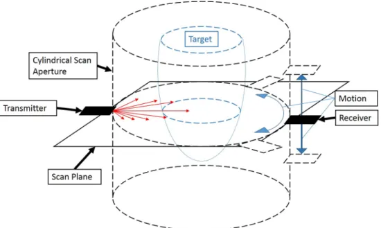
A cylindrical aperture is preferred over a semi-spherical aperture to reduce the com-plexity of the mechanical positioning system. With two single element transducers, a cylindrical aperture can be created with a combination of rotatory and linear position-ing systems (rotary tables, linear sliders, lead screw drives, etc); whereas, creatposition-ing a spherical aperture requires more complex mechanical designs (robotic arms) to define the motion axises. For imaging, the spherical system [11] overcomes the slice thickness limitations of the ring transducer system [5] by capturing out-of-plane transmissions with additional receivers. However, if the single element transducers are able to move relatively out-of-plane in a cylindrical aperture, the out-of-plane transmissions could be captured as well. The layout of a single element system in cylindrical coordinates is presented Fig. 3-1.

(30)

Figure 3-1: Cylindrical Scanning Layout

3.2 Transducers

The image quality of an acoustic scanning system is heavily dependent on the trans-ducer parameters. Particularly, the frequency and beam geometry will directly affect the depth of penetration and the image resolution, respectively. An example beam geometry of a focused single element transducer is presented in Fig. 3-2 for clarifica-tion.

(31)

3.2.1 Focus

The geometric focus point is defined by the physical curvature of the transducer lens and governs the length of the near-field, beamwidth, and beam spread [26]. The near to far-field transition locates the maxima of the transmitted acoustic wave and begins beam spreading and the decrease in wave amplitude [26]. The transducer focus should be carefully selected to ensure ample coverage of the target in the cylindrical aperture.

3.2.2 Frequency

Independent of the focus, the transducer frequency (f ) directly contributes to the im-age resolution. The wavelength (𝜆) of the transmitted wave is inversely proportional to the transducer frequency by 𝜆=c/f, where c is the speed of sound in the medium. With idealized single pulse transmissions, the best spatial resolution on the beam axis (axial resolution) is defined as 𝜆/2 [26]. For example, a 5MHz transducer scanning in water (c∼1500m/s) would have a wavelength of 𝜆=300𝜇m and an axial resolution of 150𝜇m. The resolution perpendicular to the beam axis (lateral resolution) is de-fined by the beamwidth, dependent on beam spread and the object distance from the transducer.

Frequency also affects penetration depth into the target. Attenuation of ultra-sound during propagation through a medium is frequency and distance dependent. Typical acoustic attenuation coefficients in biological tissue is shown in Table. 3.1.

Tissue Attenuation coefficient (dB/MHz/cm) Cancellous bone 10 - 40

Cortical bone 1 - 10

Fat 0.8

Muscle 0.5 - 1.5

Skin 2 - 4

Table 3.1: Attenuation coefficient of various biological tissues [14]

In comparison, bone is significantly more attenuating than soft tissue. Diagnostic ultrasound devices in soft tissue range from 2 to 15MHz in frequency, whereas clinical

(32)

bone devices range from 0.25 to 1.25MHz [14]. For the clinical motivations discussed in Chapter 1, the transducer frequency should accommodate transmission through bone without sacrificing too much spatial resolution in the muscle layers. The highest transducer frequency expected would be at 5MHz. For transmission through a 3cm thick cortical bone with average attenuation of 5dB/MHz/cm, a 5MHz signal would be attenuated by 75dB. This attenuation is high but still recoverable with current signal amplifiers. Cancellous bone may further limit the frequency but the attenuation is highly variable due to variability in the bone porosity [7]. Multiple frequency transducers may be necessary to separately accommodate each motivating clinical need.

3.3 Functional Requirements

Design Purpose: To develop a flexible tomographic acoustic imaging system that supports rapid algorithm development.

3.3.1 Primary Functional Requirements

To achieve the desired system characteristics, the following functional requirements are imposed on the system. Developed concepts should minimally satisfy the primary functional requirements to be considered.

1. Scan Aperture/Angular DOF. In sliced tomographic scanning, the transmit and receive positions must independently enclose the scan target. Corresponding to this, the system transducer transmitter and receiver positioning must form an cylindrical aperture around the scan target.

2. Axial DOF. To enable 3D volume scanning, the transducers must move axially along the length of the target.

3. Independent Motion. Transmitter and receiver positions must be independently reconfigurable to form any desired transmit receive pairing in the scan volume.

(33)

In conjunction with the angular and axial DOF requirements, the system must control four DOFs, two for each transducer. One transducer must not interfere with the other.

4. Accurate Positioning. Since image quality is directly related to transducer po-sitioning, the system must accurately position the transducers during scanning. For the target applications, the highest frequency expected is 5MHz, correspond-ing to an axial resolution of 150𝜇m. Therefore, the transducer positioncorrespond-ing error must be below 150𝜇m.

5. In-vivo Subject Scanning. System layout must allow scanning of in-vivo targets. 6. Flexible. Transducers should be easily exchangeable to enable testing of varying

transducer frequencies and beam geometries.

7. Safe. The system must be safe for human subjects. Moving mechanical compo-nents should not be in close proximity of the patient body and acoustic power of the transducers must be within FDA limits.

3.3.2 Secondary Functional Requirements

Beyond the primary functional requirements, secondary functional requirements were outlined for further evaluation of developed concepts.

1. Cost. The total system cost should be minimized. Where MRI systems could cost up to five to ten million dollars, typical ultrasound systems are ∼$150K. For a developmental system, we decided to limit our total cost to ∼$30K. 2. Simplicity. The system should not be unnecessarily complex. Concept were

evaluated in simplicity based upon the number of components, the number of custom parts, and the assembly procedure.

3. Speed. Scanning speed is important to produce images on a clinically relevant time scale. However, for a developmental system, image quality should be proven before scanning speed emphasized.

(34)

3.4 Concepts

With the primary and secondary functional requirements in mind, the following con-cepts were developed.

3.4.1 Concept A

As seen in Fig. 3-3, two large ring bearings are used to define the rotational motion while two brackets with linear sliders are used to define the axial motion. Since two independent rotations are required (transmitter and receiver), two ring bearings are necessary. For axial motion, transducer brackets with sliders and lead screws can be used to move each transducer.

Figure 3-3: Dual ring bearing

3.4.2 Concept B

Instead of using two separate bearings to define two independent rotations on the same path, Concept B uses a single track to define the path while independent carts move on the path. As shown in Fig. 3-4, the geared dual v-groove track (yellow) defines the path while two carts independently move on the track. Similar brackets

(35)

shown in Concept A can be used for axial motion.

Figure 3-4: Tracked design

3.4.3 Concept C

Instead of ring bearings, Concept C uses two small bearings below the water tank. Extension arms holding each transducer reach from the bearings into the tank. Again linear sliders can be used for vertical motion on the arms.

Figure 3-5: Dual arm design

3.4.4 Concept D

Building upon Concept C, the length of the arms can be reduced by protruding the arms through the tank base with water sealed bearings.

(36)

Figure 3-6: Through tank design

3.4.5 Concept E

Instead of moving the transducers, the entirety of the tank can be moved with the traducers attached on linear sliders.

Figure 3-7: Nested tank design

3.5 Concept Selection

Concepts were evaluated against the primary and secondary functional requirements in a weighted Pugh Matrix. Primary functional requirements were weighted more heavily to emphasize satisfaction of the overarching design purpose. Concept A was

(37)

selected as the baseline for comparison. All motion related functional requirements were grouped into "Motion" to improve clarity.

3.5.1 Summarized Pugh Chart

FRs Weight Base (A) (B) (C) (D) (E)

Motion 2 0 0 0 0 0 Accuracy 2 0 1 -2 -1 -1 In-vivo scanning 2 0 0 0 0 0 Flexible 2 0 0 0 0 0 Safe 2 0 0 -1 -2 -1 Cost 1 0 -2 -1 -2 -2 Simplicity 1 0 -1 -2 -2 -2 Speed 1 0 0 0 0 -2 Sum 0 -1 -9 -10 -10

Table 3.2: Concept Selection Pugh Chart

In comparison, all concepts satisfy the primary functional requirements, with vari-ations in accuracy and safety. Concept C and D were rated lower in accuracy since the structural path from the bearing to the transducer is longer relative to Concept A. Concept E is lower in accuracy since the inertia of the entire water tank must be moved to move the transducer; deflections are expected to be higher from heavier loading on the motion components. Concept D had the lowest rated safety due to the transducer arms at the tank bottom forming a pinch point near the scan target. Concept C and E were also lower in safety due to supporting the water tank on a smaller base and requiring to move a large mass, respectively. First order designs and reasonable cost estimates were used to compare the secondary requirements. Gener-ally, Concept C, D, and E were worse in cost and simplicity due to the number of custom components required. Speed was generally the same for all except concept E which moves a significantly higher mass.

In summary, Concept A was the best rated and Concept B was a close second. Concept B shows classical trade-off between accuracy, cost and simplicity. However, at this design size, machining of high precision components significantly increases the

(38)

overall cost. In conclusion, Concept A was selected for more further development. Concept B could be explored in the future to improve accuracy.

3.6 Summary

The functional requirements for a 3D single element tomographic system were outlined and the corresponding constraints were defined to guide the design process. Primary and secondary functional requirements were separated to better evaluate concepts. Five design concepts enabling independent transducer positioning were developed and modeled in CAD. Evaluation of the concepts against each other and the functional requirements was completed via a weighted Pugh matrix. Concept A (dual ring bearing) was selected for further development.

(39)

Chapter 4 Detailed System Design

In this chapter, we present the detailed mechanical and electrical design of the system. The necessary transducer DOFs are defined and the corresponding motion control strategy is presented. Design for each component is first presented in Solidworks, fol-lowed by the final physical prototype. Major design decisions are evaluated following the primary and secondary functional requirements and the defined design purpose. Electrical design in this chapter focuses on the motion control system; electrical design of ultrasonic data acquisition for imaging is discussed in Chapter 5.

4.1 Scanning Tank

For volumetric limb imaging, a scanning tank must hold the patient limb, two ducers, and the coupling medium. A medium is necessary acoustically couple trans-ducer to the patient limb. Ultrasound gel is used for contact probe, but for this large scale, a water tank can be used to immerse the limb and transducers. Deionized water is preferred for accurate calibrations and reducing variations in the speed of sound [1]. A 16in diameter and 7.5in long clear acrylic tube was glued (Weld-On 4) to an 0.5in acrylic plate to create the scanning tank. The cylindrical section holds the deionized water while the acrylic base serves as the system base to attach the motion structures.

(40)

4.2 Transducer Degrees of Freedoms (DOF)

In volumetric imaging, transducer DOFs are dictated by the scan aperture. In the cylindrical aperture defined in 4-1, independent angular and axial transducer DOFs are necessary. Similar to the ring transducer setup [5], arbitrary transmit and receive pairs must be possible within a single horizontal scan plane. In addition, as discussed by Hopp et al., out of plane transmit and receive pairs are necessary for reducing slice thicknesses [11]. In total, four DOFs are necessary in the system, an angular and an axial DOF for each transducer.

Figure 4-1: Scanner 3D coordinate system.

Note: Receiver position is relative to the transmitter position instead of the zero reference.

4.3 Angular Motion

To sweep circumferentially around the target, two bearings can be used to define the circular trajectory. To accommodate a patient limb transducer bracketing, and wiring, the the bearings should be around 500mm in diameter. Two options are available: geared slewing bearings and ring bearings. Slewing bearings at this scale are designed for heavy-duty applications such as: industrial machinery, aerospace and defense, and medical systems (MRI, CT). To move these heavy loads, slewing bearings are stiff and

(41)

are typically geared internally or externally for actuation. Slewing bearings provide great stiffness and accuracy but are heavy (∼100lbs) and costly (∼$4000) at the 500mm scale (www.kaydonbearings.com). For our application, loads induced from moving transducers are relatively small and do not require the high load ratings. Thin ring bearings (Lazy Susan’s) are more fitting for these smaller loads. Light and low-cost, ring bearings have both the necessary trajectory and support sufficient loads. However, these ring bearings are not geared nor typically evaluated for error motions. Additional testing and validation (Chapter 6) will be necessary to ensure positioning accuracy within the defined 150𝜇m.

(a) External geared slewing bearing

(b) Lazy Susan bearing

(42)

4.3.1 Bearing Layout

For the two transducers in the system, two ring bearings are necessary for independent angular movements. As defined in Fig. 4-1, the transmitter position (𝜃1) is relative

to the system ground, whereas the receiver angular positioning (𝜃2) is relative to the

transmitter. Therefore, the transmitter bearing must be reference the system ground while the receiver bearing must reference transmitter bearing. Shown in 4-3, the outer race of the bottom bearing is rigidly connected to the tank base (ground) while the inner races are rigidly connected to each other. In this bearing layout, the inner race of the top bearing defines angular position of the transmitter while the outer race of the top bearing defines the angular position of the receiver. This couples the two angular motions. This is acceptable since knowing receiver positioning relative to the transmitter is more important than knowing the absolute positioning of both transducers.

(43)

(44)

4.3.2 Angular Motion Control

For angular motion control, actuation of and feedback from the ring bearing is needed. Since the ring bearings are not geared, a friction pinion drive system is necessary for actuation. For the best accuracy, direct feedback on the ring bearing was chosen over indirect feedback on the drive pinion. As seen in Fig. 4-4, the friction pinion, driven by a brushless DC motor (Maxon), actuates the outer races and a high resolution (∼1𝜇m ) magnetic encoding setup (Renishaw: LM10 encoder, LM10ECL00 encoding tape) provides the feedback. Actuation and encoding for the top and bottom bearings are identical, with the exception the bottom bearing actuation is inverted to reduce space.

Figure 4-4: High resolution encoding setup and drive pinion

Closed-loop position control is implemented by an NI myRIO microcontroller in LabView. The myRIO features a customizable Xilinx FPGA in addition to the main dual-core processor. The FPGA converts the quadrature signal from the LM10 en-coder to counts and the processor samples the count on each loop-iteration. For actuation of the brushless motors, two Maxon motor drivers (Maxon PART

(45)

NUM-BER) with internal speed controllers were added. A simple proportional derivative (PD) controller implements closed-loop position control. The myRIO reads the cur-rent position on the FPGA, compares it to the desired reference, and outputs the desired motor speed to the driver. The gains are tuned to minimize overshoot to eliminate extra triggering (discussed in Chapter 5). Since the encoder tape is not absolute, a reference was marked on the bearing to zero the system during initializa-tion. Since the system is cylindrically symmetric, an arbitrary zero position can be selected. LabView VI for a single motor controller is shown in Fig. 4-5.

(46)

4.4 Axial Motion

To move transducers axially along the tank depth, two transducer brackets were designed. The bracketing should constrain five DOFs and only allow axial translation of the transducers. As seen in Fig. 4-3, the fixed-alignment linear bearing and slider shaft constrains the transducer holder in four DOFs, allowing free translation along the shaft and rotation about the shaft. To constrain rotation and add actuation, a non-captive stepper motor (HaydonKerk) was added. The non-captive motor allows movement of the threaded rod relative to the fixed motor during actuation. The non-captive stepper motor (HaydonKerk) has sufficient shaft play to self-align to the linear slider; this constrains the rotational DOF without over-constraining the holder. However, some rotational play still exists but is negligible for the small drag forces during movement through the water. Transducer bracketing is identical for both transmitter and the receiver, with the exception the receiver fixturing is shortened to adjust for placement on the top bearing inner race instead of the outer race. Holders on both brackets use band clamps to fixture the transducers. Transducers can be easily exchange and custom shapes can be 3D printed to accommodate a wide variety of transducer form factors.

(47)

4.4.1 Axial Motion Control

Since no feedback is available for the non-captive stepper motors, axial positioning is done in open-loop on the myRIO running LabView. Similar to angular motion control, an arbitrary axial position can be selected as the zero position during initialization. Dedicated stepper drivers (Pololu A4983) provide power and converts the input rising edges to steps on the motor. As shown in Fig. 4-6, the myRIO VI reads the desired number of steps from the user, then sends square wave pulses until the corresponding number of rising edges have been sent. With on/off currents in the stepper motor coils during movement, the energized coils radiate electromagnetic waves. Sufficient shielding must be present in the transducer cabling to reduce electromagnetic noise in the signal.

(48)

4.5 Summary

The fully assembled system, including the DAQ hardware is shown in Fig. 4-7.

(49)

Chapter 5 Data Acquisition Design

One of the biggest challenges in ultrasound tomography is the sheer amount of data collected in the system. For a sufficiently sampling ring or spherical breast ultrasound system, data quantities can reach up to 103GB or 97TB of data per scan, respectively [23]. Multi-transducer systems in [5] and [11] must sample all receive channels in parallel. The designed single element system only needs to sample data through one receive channel. This significantly reduces DAQ hardware cost and reduces system complexity. However, single channel streaming does not reduce the total amount of data per scan. In addition, single channel acquisition increases the total scanning time by requiring mechanical positioning of the single transducer at all receive locations and transmit locations. Nevertheless, for a cost effective algorithm development focused system, flexibility in transmitter and receiver pairing is more important than scanning speed. Scan time reduction by novel sampling strategies [25] will be explored in the future but is outside the scope of this thesis. In this chapter, we present the system data acquisition design for the single element system including: transducer selection, pulse emission, system synchronization, data sampling, and data streaming.

5.1 Transducer Selection

For calibration and initial imaging, two identical single element transducers were selected for transmission and receiving. As discussed in Chapter 3, wavelength is

(50)

inversely proportional to the frequency and defines the spatial resolution, higher fre-quency transducers are necessary to have sufficient spatial resolution to calibrate system positioning errors. We selected a 60% bandwidth (at -6dB ) 5MHz transducer for initial scanning and calibration. This frequency and bandwidth gives the best spa-tial resolution while maintaining emission of lower frequency bands for transmission through bone.

To enable testing of tomographic methods such as ray-tracing or attenuation map-ping, wide beamwidth or omni-directional transducers are needed. For these methods, the transmitted beam front should cover the smallest boundary circle (BC) enclosing the target cross section at the center of the tank. With the frequency and beamwidth specification, we selected the Olympus V308-SU transducer with focus at 1in for ini-tial testing (Figure 5-1b). Transducers are easily exchangeable on the holder; various frequencies and beam geometries can be tested in the future.

(a) BC enclosed by a wide beamwidth transducer

(b) Focused single element 5MHz trans-ducer

Figure 5-1: Focused 5MHz transducer and the enclosed BC

5.2 Pulser/Receiver

For ultrasound transmission and reception, a low frequency pulser/receiver (JSR Ul-trasounics DPR300) was selected. The DPR300 shock excitation pulser/receiver is switchable between pulse-echo and pitch catch modes, and has flexibility in the

(51)

trans-mit pulse duration, pulse amplitude, damping, and control over the receive amplifi-cation and filtering.

5.3 High Speed Data Acquisition

As previously discussed, total data quantities can reach many gigabytes. Typical scopes have do not hold sufficient on-board memory to accommodate such large data quantities. High speed transfer from the scope to a host PC is necessary to prevent data loss.

5.3.1 Data Rate

A first-order estimate of data rates in a single slice pulse-echo scan was used to estimate necessary data transfer rates. For a 5MHz transducer sampled 50MHz with 14-bit resolution, a single pulse-echo amplitude modulation scan (A-scan) of a 500mm diameter tank would produce 43.7kB of data. Scanning the 500mm diameter circular aperture with 𝜆/2 (150𝜇m) sampling resolution produces 10467 A-scans. Reasonably limiting a single slice pulse-echo sequence to 5 seconds, each sweep generates about 90MB/s. This data rate is significantly higher than the maximum transfer speeds of USB 2.0 DAQs interfaces (60MB/s). PCI Express bus (500MB/s) based DAQs are necessary to accommodate these high data rates. (Note: USB 3.0 DAQs are sufficient and available but were not selected due to similar pricing for slower data transfer speed when compared to PCI Express)

5.3.2 Digitizer

For ease of system integration in LabView, a high speed NI digitizer card (PXIe-5122) was selected to sample data output from the DPR300 pulser/receiver. In addition, the designed NI PXI chassis incorporates a PCI Express link to the host PC (PXIe-8270), ensuring high data transfer speeds. The PXIe-5122 provides 14-bit sampling resolution up to 100MHz maximum.

(52)

5.4 Synchronization

For data acquisition timing, all components of the system must be synchronized to when the ultrasound transmitting transducer is triggered on the DPR300. In fixed height pulse-echo scanning with uniform sampling, the transducer must emit and receive pulses at fixed angular increments around the scan object. In pitch-catch mode, the transmitter must emit when the receiver has moved a fixed angular increment. Regardless of scanning mode (pulse-echo for backscatter scanning or pitch-catch for tomographic scanning), the system should be triggered based upon the location of the transducer with respect to the desired sampling resolution. Angularly, the trigger signal will be dependent on the encoder count. Axially, the trigger signal will be dependent on the step number. Both the encoder count and the step number is recorded within the myRIO. When the trigger condition of the count or step increment is met, the myRIO control virtual instrument (VI) will automatically send a square wave pulse to trigger both the DPR300 and the PXIe-5122.

On the myRIO, the desired step and count increments between each trigger are set before control is initiated. Axial triggering based on the step increment is done directly in the main control VI; however, angular triggering is done on the FPGA. Due to the high encoder resolution (1𝜇m), the encoder count on the FPGA changes significantly faster (40MHz ) than how fast the control VI can sample (1kHz ). If the trigger condition is dependent on the count sampled by the control VI, many angular triggers would be missed. To eliminate the sampling discrepancy, the angular triggering is directly implemented in hardware on the FPGA. As shown in Fig. 5-2, the myRIO FPGA VI first converts the LM10 quadrature output to counts; if the count is matches the trigger condition, the square wave trigger pulse will sent. An additional line driver (Texas Instruments CD74AC244E) was added on the myRIO trigger output to supply sufficient power to drive the DPR300 and the PXIe-5122 trigger inputs. Full layout of the data acquisition schematic is shown in Fig. 5-3 (line driver not shown).

(53)

Figure 5-2: Custom FPGA personality for high speed triggering

(54)

5.5 Summary

A 5MHz transducer has been selected for initial testing of the system. To accom-modate expected data rates and volume, a high speed DAQ hardware was designed, assembled, and synchronized to the encoder position count on the FPGA which is recording transmit location.

(55)

Chapter 6 System Characterization

Variations and error in the mechanical assembly, transducer characteristics, and data sampling all contribute to degradation and error in the final image quality of the system. Each of these error sources must be accounted for to evaluate and correct for aggregate errors in the system. In this chapter, we present a characterization of the error sources including transducer positioning errors, DAQ instabilities, and speed of sound (SoS) variations. In addition, the actual transducer beamwidth was simulated in a finite element (FE) software (PZflex) and measured to quantify the actual covered ROI.

(56)

6.1 Error Sources

To establish a ground truth, calibration fixtures of known geometry (cylindrical rods/threads) fastened at fixed locations on the threaded calibration plate (Fig. 6-1) were scanned (pulse-echo, 5MHz transducer).

Figure 6-1: 0.5in nylon 6-6 rod centered in the tank on the calibration plate. Using the coordinate system defined in Fig. 4-1, the position of a scatterer in pulse-echo scanning in a single horizontal plane is

𝑠(𝜃) = 𝑅(𝜃) − 𝐶 * 𝑡(𝜃)/2 (6.1)

For each angular position 𝜃, 𝑠 is the distance of a scatterer from the center of the tank, 𝑅 is the radial position of the transducer, 𝐶 is SoS, and 𝑡 is the two-way travel time of the received echo. To separate error contributions from each input, partial derivatives of Eq. 6.1 with respect to each variable is analyzed to define an error budget for each respective input. Total alloted error is bounded by the minimum acoustic resolution of 150𝜇m (5MHz ). 𝑑𝑠 = 𝜕𝑠 𝜕𝑡𝑑𝑡 + 𝜕𝑠 𝜕𝑅𝑑𝑅 + 𝜕𝑠 𝜕𝐶𝑑𝐶 ≤ 150𝜇m (6.2)

(57)

Following Eq.6.2, the total error is the summation of each partial derivative mul-tiplied by the respective deviation. To satisfy the total 150𝜇m alloted error, equal 50𝜇m contribution is alloted for each input. Using expected mean values for each pa-rameter, reasonable error bounds can be defined for each input. With expected SoS in water around 1500m/s [1] and maximum travel time around 200𝜇s in the scanning aperture, the following bounds can be established.

Partial Estimate Bounds Source

𝜕𝑠 𝜕𝑡𝑑𝑡 =

𝐶

2𝑑𝑡 C≈1500m/s 𝑑𝑡 ≤ 67𝑛𝑠 DAQ instability 𝜕𝑠

𝜕𝑅𝑑𝑅 = 1𝑑𝑅 None 𝑑𝑅 ≤ 50𝜇m Position error 𝜕𝑠

𝜕𝐶𝑑𝐶 = 𝑡

2𝑑𝐶 t𝑚𝑎𝑥≈200𝜇s 𝑑𝐶 ≤ 0.5𝑚/𝑠 SoS variation

(58)

6.1.1 DAQ Stability

To characterize the DAQ sampling measurement stability, 2000 pulse echo A-scans were captured with the transducer and the target at a fixed separation. Temporal location of the first echo envelope peak was detected, shifts in the peak location within the 2000 A-scans were recorded to characterize DAQ stability. Measurements were repeated 9 times at varying separations.

Figure 6-2: DAQ Stability.

The maximum temporal shift in peak location is only 1 sampling interval, corre-sponding to 20ns, lower than the alloted 67ns time error. For expected SoS around 1500m/s, final position error due to time sampling would be 30𝜇m.

6.1.2 Radial Positioning Error

Similar to the calibration procedure for ring arrays [28], the radial position error of the transducer is quantified by recording A-scans at 1533 angular positions around a known target (0.5075in (12.9mm) diameter nylon 6-6 rod). With a known SoS in the medium, temporal deviations in the first echo peak can be characterized as the radial

(59)

position error of the transducer at each angular position. 9 A-scans were collected at each angular position.

Figure 6-3: Mechanical Positioning Error.

As seen in Fig. 6-3, radial position of the transducer shows ∼±30𝜇m deviations at each angular position. Maximum and minimum errors at each position was shifted by 1mm to improve clarity (Fig. 6-3 top). The sinusoidal presence in Fig. 6-3 will be discussed in Chapter 7 and is due to the slight non-centered positioning of the nylon rod in the tank. The presented radial error includes the previously evaluated DAQ stability error. However, though inclusive, the total error is still lower than the 50𝜇m alloted.

6.1.3 Speed of Sound Error

For system characterization in pulse-echo, the SoS is assumed to be global and con-stant within the imaging volume. Since SoS is temperature dependent and varia-tions are small in deionized water [1], accurate measurement (±0.1∘C) of

(60)

tempera-ture can be used to compensate for temperatempera-ture deviations. Water temperatempera-ture was measured with a precision thermometer (ThermoWorks-Precision Plus Thermometer) with ±0.05∘C accuracy before each scan.

6.2 Beamwidth Characterization

As discussed in Chapter 5 in Fig. 5-1a, a wide beamwidth transducer is necessary to cover a ROI in the center of the scanning tank. The focused 5MHz transducer was simulated in PZFlex to estimate the ROI coverage size in the tank center. As seen in Fig. 6-4, the beam pattern shows a 62∘ beam width for the focused transducer. At the center of the tank, the ROI covered would be about ∼4.9in in diameter. This beam width was validated with transmission scans on an empty water tank. A fixed transmitter was pulsed as the receiver scanned around the water tank. The simulated and measured beamwidths are shown in Fig. 6-4 and below.

(a) PZFlex Simulation (b) Power profile at 20cm

Figure 6-4: Simulated transducer beam pattern.

At 20mm distance from the face of the transducer (the center of the cylindrical aperture), the simulated beam pattern shows a 62∘ beamwidth, while the measured beam profile in the empty tank showed 61∘. Discrepancies in the power profile can be attributed to the measuring receiver moving in a circular arc while the simulation profile is a linear cut at 20cm. Overall, the simulation and measurement beamwidth

(61)

(a) Measured beam pattern (b) Power profile

Figure 6-5: Measured transducer beam pattern.

show sufficient agreement to validate the transducer beamwidth, corresponding to a ∼4.8in ROI at the center of the scanning tank.

6.3 Summary

To obtain the best image quality, error sources relevant to accurate localization of scatterers in the tank has been tracked and characterized. The total error budget established from the functional requirements was evaluated against the measured error values. The measured errors were within the defined 50𝜇m error boundaries. The beamwidth of the focused 5MHz transducer was simulated and measured and showed sufficient size to cover a 4.8in ROI at the center of the tank.

(62)

Chapter 7 Echo Imaging

In this chapter, we present single element pulse-echo image reconstruction of various targets inside the scanning tank. A-scans at each angular position combined to form a cross-sectional B-mode (amplitude scaled brightness) image of the scan target; axial B-mode slices were produced similarly. Image distortions from the receiver angular insensitivity were corrected with a migration algorithm. Raw B-mode and corrected images are both presented in the chapter. Water temperature was measured in the distilled water before each scan to account for deviations in the speed of sound.

(63)

7.1 Fixed Height Echo Imaging

Tracing the circular path defined by the ring bearing, the focused 5MHz wide beam transducer was used for pulse-echo imaging of various targets at fixed axial heights. A-scans at 1533 angular positions (0.235∘ angular resolution) with 20000 samples (50MHz sampling rate, 14-bit resolution) were combined to produce B-modes slices of scan targets. B-mode images of two cylindrically symmetric objects, centered in the tank, are shown in Fig. 7-1.

(a) 0.5in nylon 6-6 rod (b) Phantom with 0.5in nylon rod

Figure 7-1: B-mode images of centered cylindrically symmetric objects

Reflections from the object boundaries are clearly seen. Multilayer propagations through the co-polymer phantom [20] show sufficient echo power to image internal embedded structures.

(64)

7.2 Image Distortion

As targets move off-center in tank, reconstructed images show significant distortions in size and shape. As shown in Fig. 7-2, off-center scatterers appear as circular doublets in polar images (Fig. 7-2c and 7-2d) and sinusoids in Cartesian images (Fig. 7-2a and 7-2b). Fig. 7-2b is in grayscale to improve contrast.

(a) Two 0.5in Nylon 6-6 rods (Cartesian) (b) Single off-center nylon thread (Carte-sian)

(c) Two 0.5in Nylon 6-6 rods (Polar) (d) Single off-center nylon thread (Polar)

Figure 7-2: Object distortions in Cartesian and Polar coordinates

(65)

dis-cussed in Chapter 6 to cover a ROI, a wide beamwidth is necessary. However, for a focused single element transducer, the receive aperture is directionally insensitive. As discussed by Norton et al. [17], in a circular aperture, each point in a A-scan line actually corresponds to the sum of the echo response from all scatterers along a circu-lar arc centered at the transducer location [17]. This wide beam angucircu-lar insensitivity creates distortions for off-center scatterers in the tank.

Figure 7-3: Angular Insensitivity of a omni-directional source

As shown in Fig. 7-3, echoes from off angle scatterers will appear directly in-line with the transducer face. However, because the transducer position is known, the expected distorted shape for every point scatterer in the image can be calculated (Eq. 7.1). For example, a point scatterer at 𝜃=0∘ and r=60mm scanned in 360∘ pulse-echo with an omni-directional source would produce the (distortion) profile shown in Fig. 7-5d.

(66)

Figure 7-4: Defined transducer (R) and point scatterer (P) coordinates for Eq. 7.1

𝑑 =√︁(𝑅2

𝑟 + 𝑅2𝑝− 2𝑅𝑟𝑅𝑝𝑐𝑜𝑠(𝜃𝑟− 𝜃𝑝) (7.1)

(a) 0-90∘ _{(b) 0-180}∘ _{(c) 0-270}∘ _{(d) 0-360}∘

Figure 7-5: Profile of a point scatterer at (0,60mm) viewed in pulse-echo by an omni-directional source/receiver moving in a circular aperture

Since the distortion profile is known for every point inside the scan plane, each distortion profile can be used to sum and migrate echoes for image correction.

7.3 Image Correction Algorithm

From Eq. 7.1, each calculated distortion profile gives the spatial location of the echoes associated with a single point source. In Cartesian coordinates, calculated point scatterer present as sinusoids, in polar coordinates, circular doublets, as shown in Fig. 7-5. This is in agreement with the appearance of the scanned nylon thread (Fig. 7-2d).

(67)

For image correction, expected distortion profiles are calculated for every point inside the scan plane. Line integrals along the distortion profiles sum the associated echoes for every point. Summation results from each line integral define the echo strength for each point. This operation can be thought of as accumulating echoes from appropriate A-scans points and moving the summation to the proper location in space. This image correction technique is based on the reflectivity tomography algorithm by Norton [18]. The algorithm is valid for a monostatic setup with an omnidirectional transducer which travels in a circular path and insonifies targets that are weak and omnidirectional scatterers. Flow chart for the image correction algorithm is presented in Fig. 7-6.

(68)

(69)

7.3.1 Corrected Images

Corrected B-mode images of the nylon rods and thread are shown in Fig. 7-7.

(a) Corrected two nylon rods (b) Corrected off-center nylon thread

Figure 7-7: Correct images after migration

The algorithm correctly recovers the expected shapes and sizes of the scanned targets. Previously distorted nylon rods show with corrected sizes and locations (Fig. 7a) and the nylon thread shows as a point scatterer as expected (Fig. 7-7b). However, the algorithm does add noise to the image at the scatterer boundaries. This is a result of the finite axial resolution of the transducer and deviations from the original assumptions of the algorithm.

7.4 Fixed Angle Echo Imaging

In addition to the fixed plane images, A-lines from axial scans were combined to produce axial B-mode slices. Axial pulse-echo scanning is mathematically identical to scanning with a linear array probes. Based the array sampling theory, the maximum sampling resolution should be less than 𝜆/2 (150𝜇m at 5MHz ) to prevent grating lobes in real space [26]. Correspondingly, axial scans used 40 step increments (127𝜇m) between triggers. Axial scans of the a steel calibration rod and the rod with an added

(70)

steel collar is shown in Fig. 7-8. An image of the scan setup is presented in Fig. 7-10.

(a) Steel rod (b) Steel rod with collar

Figure 7-8: Vertical steel rod scans

The same image distortion is present in axial scanning as is present in angular scanning. Similar image correction algorithm can be applied in axial scanning with adjustments to the line integrals. In the vertical rectangular plane, the line integral path becomes the Euclidean distance between the transducer and the scatterer, as the transducer is moved.

𝑑 =√︁(𝑅𝑟− 𝑅𝑝)2+ (𝑉𝑟− 𝑉𝑝)2 (7.2)

Corrected images are shown in Fig. 7-9.

(a) Corrected steel rod (b) Corrected steel rod with collar

(71)

7.4.1 Axial Scan Resolution

Identical to the lateral resolution of linear arrays, the axial scan resolution is defined by the beamwidth of the transducer. With a 61∘ beamwidth, at the center, the lateral resolution would be 4.8in. Axial B-mode images show the smearing due to the large axial resolution; two separated steel collars merge into a single body in the axial scans. Steel collars at various separations attached on the steel rod are shown in Fig. 7-11. However, the image correction process improves the lateral resolution and better differentiates the collars at different separations, particularly when comparing Fig. 7-11c and Fig. 7-11d.

The axial scan resolution is critical because it directly affects slice thickness in pulse-echo imaging. Though the image correction algorithm improves the resolution, further improvements can be made by using a non-spherically focused transducer in the future.

(72)

(a) 0mm (b) Corrected 0mm

(c) 10mm (d) Corrected 10mm

(e) 20mm (f) Corrected 20mm

(g) 30mm (h) Corrected 30mm

(73)

7.5 Bone Scans

Angular and axial B-mode images of a lamb long bone, immersed in the scanning tank, is presented in Fig. 7-15 and Fig. 7-16. Previously discussed angular and axial image corrections were implemented on the images to generate each figure.

The outer bone surfaces are clearly seen along with limited view of the internal structures. Cortical bone thickness can be seen at surfaces directly perpendicular to the transmitted wave. Limited penetration depth due to attenuation of the 5MHz signal is expected in the bone [14]. With the transducer bandwidth, lower transmitted frequencies (∼500kHz ) have some penetration into the bone, showing the cortical bone thickness when the incident wave is perpendicular to the bone surface. In future development, lower center frequency transducers should provide better penetration depth into the bone.

(74)

Figure 7-13: Lamb long bone at viewed at various angles

(75)

Figure 7-15: Angular scan of a lamb long bone

(76)

7.6 Human Forearm

First in-vivo scanning in the system was completed on a human forearms in the scanning tank. Subjects placed their palm flat on the tank base while the transducer scanned circumferentially around the mid forearm. B-mode images before and after image correction are shown in Fig. 7-17 below.

(a) Forearm with motion (b) Forearm with reduced motion

Figure 7-17: Forearm angular scans

In Fig. 7-17b, the skin and bone surfaces are clearly seen after image correction. However, Fig. 7-17a shows severely disconnected structures with or without image correction. This discontinuity is due to movement of the forearm during the scan. This is in agreement with findings from Douglas et al. [4]; involuntary patient movement during ultrasound scanning of lower limbs heavily affect the image quality. Initial imaging of human limbs show promise in capturing the skin and bone surface contours. Additional scan subjects, ground truth comparison with MRI images, and motion compensation algorithms are necessary for further system development.

Design of a single element 3D ultrasound scanner

Design of a Single Element 3D Ultrasound Scanner

by

Xiang Zhang

B.S. University of Maryland (2013)

Submitted to the Department of Mechanical Engineering

in partial fulfillment of the requirements for the degree of

Master of Science in Mechanical Engineering

at the

MASSACHUSETTS INSTITUTE OF TECHNOLOGY

June 2015

c

○ Massachusetts Institute of Technology 2015. All rights reserved.

Author . . . .

Department of Mechanical Engineering

May 8, 2015

Certified by . . . .

Brian W. Anthony

Principal Research Scientist, Department of Mechanical Engineering

Thesis Supervisor

Accepted by . . . .

David E. Hardt

Graduate Officer, Department of Mechanical Engineering

Design of a Single Element 3D Ultrasound Scanner

by

Xiang Zhang

Abstract

Acknowledgments

Contents

List of Figures

List of Tables

Chapter 1

Introduction

1.1

Clinical Motivation

1.1.1

Prosthetic Fitting

1.1.2

Bone Mineral Density Monitoring

1.1.3

Muscle Deterioration Monitoring

1.2

Thesis Scope

Chapter 2

Ultrasound Tomography

2.1

Soft Tissue Ultrasound Tomography Systems

2.1.1

Ring Arrays

2.1.2

Conical Arrays

2.1.3

Array Probe Scanner

2.2

Single Element Scanning

2.3

Summary

Chapter 3

System Requirements

3.1

Single Element Scanning Layout

3.2

Transducers

3.2.1

Focus

3.2.2

Frequency

3.3

Functional Requirements

3.3.1

Primary Functional Requirements

3.3.2

Secondary Functional Requirements

3.4

Concepts

3.4.1

Concept A

3.4.2

Concept B

3.4.3