Antarctic-like temperature variations in the Tropical Andes recorded by glaciers and lakes during the last deglaciation

HAL Id: hal-03029770

https://hal.univ-lorraine.fr/hal-03029770

Submitted on 2 Dec 2020

HAL is a multi-disciplinary open access

archive for the deposit and dissemination of sci-entific research documents, whether they are pub-lished or not. The documents may come from teaching and research institutions in France or abroad, or from public or private research centers.

L’archive ouverte pluridisciplinaire HAL, est destinée au dépôt et à la diffusion de documents scientifiques de niveau recherche, publiés ou non, émanant des établissements d’enseignement et de recherche français ou étrangers, des laboratoires publics ou privés.

Distributed under a Creative Commons Attribution - NonCommercial - NoDerivatives| 4.0 International License

Antarctic-like temperature variations in the Tropical

Andes recorded by glaciers and lakes during the last

deglaciation

L. Martin, P.-H Blard, J Lavé, V. Jomelli, J. Charreau, T. Condom, M.

Lupker, Maurice Arnold, Georges Aumaitre, D.L. Bourlès, et al.

To cite this version:

L. Martin, P.-H Blard, J Lavé, V. Jomelli, J. Charreau, et al.. Antarctic-like temperature variations in the Tropical Andes recorded by glaciers and lakes during the last deglaciation. Quaternary Science Reviews, Elsevier, 2020, 247, pp.106542. �10.1016/j.quascirev.2020.106542�. �hal-03029770�

Antarctic-like temperature variations in the Tropical Andes

1

recorded by glaciers and lakes during the last deglaciation

2

L.C.P. Martina,b*_{, P.-H. Blard}a,c*_{, J. Lavé}a_{, V. Jomelli}d,e_{, J. Charreau}a_{, T. Condom}f_{, M. Lupker}g_,

3

ASTER Teame#

4

a. CRPG, UMR7358 CNRS - Université de Lorraine, 54500 Vandœuvre-lès-Nancy, France

5

b. Department of Geosciences, University of Oslo, P.O. Box 1047, Blindern, 0316 Oslo, Norway

6

c. Laboratoire de Glaciologie, DGES-IGEOS, Université Libre de Bruxelles, 1050 Brussels, Belgium

7

d. Université Paris 1 Panthéon-Sorbonne, CNRS Laboratoire de Géographie Physique, Meudon, France

8

e. Aix-Marseille Université, CNRS-IRD-Collège de France-INRAE, UM 34 CEREGE, Aix-en-Provence,

9

France

10

f. Université Grenoble Alpes, CNRS, IRD, G-INP, Institut des Geosciences de l’Environnement (IGE) –

11

UMR 5001, Grenoble, France

12

g. ETH, Geological Institute, Sonneggstrasse 5, 8092 Zurich, Switzerland

13

# M. Arnold, G. Aumaître, D. L. Bourlès, K. Keddadouche

14

* Corresponding authors:

15

leo.doug.martin@gmail.com; blard@crpg.cnrs-nancy.fr

16

Centre de Recherches Pétrographiques et Géochimiques

17

15 rue Notre Dame des Pauvres

18

19

20

21

22

23

- Supplementary Information: 1,247 words, 3 Tables,4 figures

24

Keywords: paleoclimate dynamics; Tropical Andes; paleoglaciers; cosmogenic nuclides; 10_Be, 3_He;

25

glacial geomorphology; last deglaciation; Termination 1; continental paleotemperature and precipitation

26

reconstruction, global and regional climate.

Highlights

28

- Cosmic ray exposure ages and paleo-ELAs determined for Bolivian Andes late-glacial moraines

29

- New 14_{C shoreline ages constrain the depth of paleolake Coipasa (12.5 cal kyr BP)}

30

-

31

-

32

-

33

Abstract

34

The respective impacts of Northern and Southern Hemispheric climatic changes on the Tropics

35

during the last deglaciation remain poorly understood. In the High Tropical Andes, the Antarctic Cold

36

Reversal (ACR, 14.3-12.9 ka BP) is better represented among morainic records than the Younger Dryas

37

(12.9-11.7 ka BP). However, in the Altiplano basin (Bolivia), two cold periods of the Northern

38

Hemisphere (Heinrich Stadial 1a, 16.5-14.5 ka BP, and the Younger Dryas) are synchronous with (i)

39

major advances or standstills of paleoglaciers and (ii) the highstands of giant paleolakes Tauca and

40

Coipasa.

41

Here, we present new cosmic ray exposure (CRE) ages from glacial landforms of the Bolivian

42

Andes that formed during the last deglaciation (Termination 1). We reconstruct the equilibrium line

43

altitudes (ELA) associated with each moraine and use them in an inverse algorithm combining

44

paleoglaciers and paleolake budgets to derive temperature and precipitation during the last deglaciation.

45

Our temperature reconstruction (ΔT relative to present day) yields a consistent regional trend of

46

progressive warming from ΔT = –5 to –2.5 °C during 17–14.5 ka BP, followed by a return to colder

47

conditions around –4°C during the ACR (14.5-12.9 ka BP). The Coipasa highstand (12.9-11.8 ka BP)

48

is coeval with another warming trend followed by ΔT stabilization at the onset of the Holocene (ca. 10

49

ka BP), around –3°C. Our results suggest that, during the last deglaciation (20 – 10 ka BP) atmospheric

50

temperatures in the Tropical Andes mimicked Antarctic variability, whereas precipitation over the

51

Altiplano was driven by changes in the Northern Hemisphere.

1. Introduction

53

The last deglaciation was characterized by major reorganizations of the continental and oceanic

54

climate systems, including modifications of oceanic circulations (McManus et al., 2004), and the

55

monsoon systems (Cruz et al., 2005), shifts of the wind belts (Denton et al., 2010; Toggweiler, 2009),

56

and opposing north/south temperature variations (Barker et al., 2009; Broecker, 1998). During this

57

period, antiphase warming/cooling events (such as the Northern Hemisphere, NH, warm

Bølling-58

Allerød and the Southern Hemisphere, SH, Antarctic Cold Reversal, Andersen et al., 2004; Jouzel et al.,

59

2007) may have influenced both hemispheres and triggered major continental hydro-climatic changes

60

(e.g. Barker et al., 2011; Blard et al., 2011a, 2009; Broecker and Putnam, 2012; Jomelli et al., 2014;

61

Martin et al., 2018; Placzek et al., 2006; Sylvestre et al., 1999). However, the respective

62

interhemispheric impacts of oceanic and atmospheric changes remain controversial and the subject of

63

various investigations (e.g. Blard et al., 2009; Fritz et al., 2007; Jomelli et al., 2014).

64

Because the tropics are intersectional between the Northern and Southern Hemispheres, this

65

region is key to addressing the respective impacts of both hemispheres on global and regional climates

66

(Jackson et al., 2019). The Tropical Andes, and particularly the Altiplano Basin, exhibit outstanding

67

hydro-climatic archives of climatic changes during the last deglaciation. Indeed, the Antarctic Cold

68

Reversal (a SH event) was reported to have exerted a major influence on glacial dynamics throughout

69

the tropical and sub-tropical Andes (Jomelli et al., 2014). Furthermore, in the Altiplano,

paleo-70

highstands of Lakes Tauca (52,000 km2_{) and Coipasa (32,000 km}2_{) are synchronous with the second}

71

half of the Heinrich Stadial 1 (16.5 – 14.5 ka BP) and the Younger Dryas (12.9 – 11.7 ka BP),

72

respectively (NH events, Blard et al., 2011a; Placzek et al., 2006; Sylvestre et al., 1999). These lake

73

cycles are characterized by abrupt transgressions and regressions within 1 kyr, implying drastic and fast

74

climatic changes that occurred synchronously with abrupt changes within the northern Atlantic region

75

(Andersen et al., 2004; McManus et al., 2004). Throughout the Altiplano Basin, moraine records

76

evidence glacial standstills or re-advances synchronous with the Lake Tauca highstand, which Martin

77

et al. (2018) used to reconstruct the regional distribution of precipitation during Heinrich Stadial 1 (16.5

78

– 14.5 ka BP), for which they computed a regional precipitation increase of 130% (i.e. a factor of 2.3).

Relying on their reconstructed spatial distribution of precipitation, they concluded that the change in

80

rainfall regime during Heinrich Stadial 1 resulted from modifications of the South American Summer

81

Monsoon (SASM), involving a southward shift of synoptic atmospheric features compared to the

82

present.

83

Numerous studies have provided local chronologies of glaciers fluctuations in the tropical

84

Andes for the last glacial maximum (LGM) and late-glacial period (e.g. Bromley et al., 2016; Carcaillet

85

et al., 2013; Farber et al., 2005; Palacios et al., 2020; Shakun et al., 2015; Smith, 2005; Ward et al.,

86

2015; Zech et al., 2009) and climatic reconstructions from glacial landforms in the vicinity of the

87

Altiplano have already been reported (Jomelli et al., 2011; 2016, Kull et al.,, 2008; Kull and Grosjean,

88

2000; Malone et al., 2015). In the Altiplano, Blard et al. (2009) and Placzek et al. (2013) quantified

89

temperature variations based on joint lake- and glacier-budget calculations during the Lake Tauca cycle.

90

However, these previous approaches suffered from substantial uncertainties on the spatial distribution

91

of precipitation over the Altiplano because very few climatic reconstructions are available before and

92

after the Lake Tauca highstand. Notably, little is known about Tropical Andean temperatures and

93

precipitation during the LGM-Heinrich 1 transition, the ACR and the Younger Dryas. In this regard,

94

climatic reconstructions spanning the last deglaciation in the High Tropical Andes are critical to

95

establishing the extent and influence of these major and potentially opposing climatic changes recorded

96

at high latitudes of the Northern and Southern Hemisphere.

97

Here we present new glacial chronologies from four sites of the Bolivian Altiplano: the Zongo

98

valley (16.3°S, 68.1°W), Nevado Sajama (18.1°S, 68.9°W), Cerro Tunupa (19.8°S, 67.6°W), and Cerro

99

Luxar (21.0°S, 68.0°W). These chronologies are based on cosmic ray exposure (CRE) dating of

100

recessional moraine sequences and glacially abraded bedrock surfaces. These new data extend the

101

existing chronologies of Smith et al. (2005), Jomelli et al. (2011), Blard et al. (2009, 2013) and Martin

102

et al. (2018). Considering lake-level variations over the same period, we applied an inversion method

103

that builds on our previous studies (Blard et al. 2009, Martin et al. 2018). By coupling glacier- and

lake-104

budget calculations, we took advantage of their contrasting sensitivities to temperature and precipitation,

105

and reconstructed temperature and precipitation ranges that jointly satisfy glacial and lacustrine extents

106

for a given moment of the last deglaciation.

2. Geological Setting

108

2.1. Climate of the Altiplano

109

The Altiplano is a wide intra-mountain plateau covering an area of 196,000 km2 _{and bounded}

110

by the eastern and western Andes Cordilleras (Fig. 1). Due to its regional topography, this area is an

111

endorheic basin (hereafter, the “Altiplano Basin”). This basin extends from 15.5°S (Peru) to 22.5°S

112

(Bolivia), and ranges in elevation from 3,658 m above sea level (asl) at Salar de Uyuni to 6,542 m asl

113

at Sajama volcano.

114

The precipitation regime of the Altiplano is under the climatic influence of the SASM, which

115

brings most of the annual rainfall during the austral summer (December, January, February, Vera et al.,

116

2006; Zhou and Lau, 1998). During this period, the dry westerlies are weakened by subtropical jet

117

modulations and a concomitant southward expansion of the tropical easterlies. This modification

118

promotes the transport of humidity from the Amazonian basin and central Brazil towards the Altiplano

119

(Garreaud et al., 2003, 2009; Segura et al., 2019; Vuille, 1999; Vuille and Keimig, 2004). The

120

orographic effect of the Eastern Cordillera modulates this transport and creates an important

121

precipitation gradient over the Altiplano. Annual rainfall presently ranges from 800 mm on the shores

122

of Lake Titicaca to 60 mm in the vicinity of the Laguna Colorada, southwest Bolivia (Fig. 1).

123

Present temperatures are relatively uniform over the Altiplano, and the daily temperature

124

variability is larger than the seasonal variability (Aceituno, 1996) as is often observed in the tropics

125

(Hastenrath, 1991). Maximum daily temperatures occur around 2 pm LT when solar radiation is

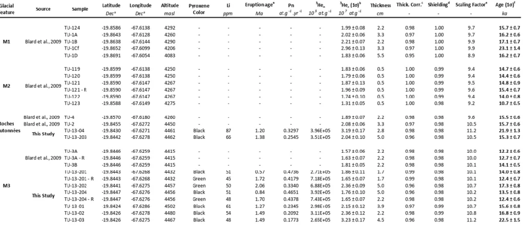
126

maximal. For most of the year, daily temperature variations are constrained by night radiative loss from

127

the surface. Therefore, the daily amplitude of temperature variations is reduced during the wet season

128

when cloudiness is important (Condom, 2002). Climatic conditions at the glacial sites are presented in

129

Table 1.

131

Figure 1. South American climate and the Altiplano Basin. (A) Modern features of the South American

132

climate, with particular focus on the summer monsoon. SWW, southern westerly winds; AMOC, Atlantic

133

meridional overturning circulation; ITCZ, intertropical convergence zone; SALLJ, South American

134

low-level jets; SACZ, South Atlantic convergence zone; BH, Bolivian High. The colored background

135

indicates mean annual rainfall (*color scale truncated at 3,500 mm). Blue contours show the

136

December–February (DJF) to annual precipitation ratio. Precipitation data are mean values during

137

1979–2016 from ERA-Interim (Dee et al., 2011). (B) The Altiplano Basin and the locations of sites

138

analyzed herein overlaid on SPOT Imagery. White dots indicate glacial valleys, and the red dot indicates

139

lacustrine deposits sampled and analyzed herein. The maximum paleo-extent of Lake Tauca is shaded

140

in blue. The black line delimits the Altiplano endorheic basin.

141

2.2. Altiplano hydrology and paleolake records

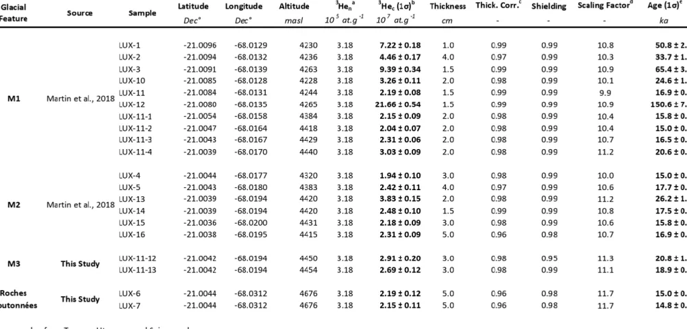
142

The Altiplano endorheic basin comprises a north-south succession of four adjacent sub-basins

143

(Fig. 2). The Titicaca watershed in the northern Altiplano is the highest (lake altitude, 3,812 m asl) and

144

wettest sub-basin. It drains to the southeast via Rio Desaguadero (Figs. 1 and 2) to the Poopo watershed.

145

Lake Poopo was a shallow lake (<3 m deep) that vanished in 2015 due to ongoing climate change and

146

excessive irrigation (Satgé et al., 2017). The small Coipasa watershed is to the southwest of Poopo

147

watershed, and the two are separated by an elevation threshold of 3,703 m asl (Fig. 2). The Uyuni

148

watershed (bottom at 3,660 m asl) is to the south of Coipasa watershed, from which it is separated by

149

an elevation threshold of 3,672 m asl. Channels and paleochannels between the different basins indicate

150

that they were hydrologically connected during wetter periods.

152

Figure 2. Topographic cross section of the Altiplano showing the hydrological relationships between

153

lake and salar watersheds (modified from Argollo and Mourguiart, 2000). The threshold between the

154

Poopo and Coipasa watersheds is 3,703 m asl. The threshold between the Coipasa and Uyuni

155

watersheds is 3,672 m asl. The elevation reported for paleolake Coipasa is based on our new shoreline

156

14_{C ages (see Section 4.1.1).}

157

158

The three southernmost basins of the Altiplano are dry at present, but were covered by large

159

lakes during the wettest periods of the Quaternary (Placzek et al., 2006; Sylvestre et al., 1999). Of the

160

several lake episodes that occurred during the last 120 kyr, the Lake Tauca episode was the widest and

161

deepest (110 to 120 m deep, Placzek et al., 2006; Blard et al., 2011). During the Lake Tauca highstand

162

(3,770 m asl), the lake extent covered the totality of the three southernmost basins (Poopo, Coipasa and

163

Uyuni; Figs. 1 and 2).

164

U-Th and 14_{C dating of its shorelines constrain the timing of the Lake Tauca cycle, i.e. the}

165

transgression (18-16.5 ka BP), highstand (16.5-15.5 ka BP) and regression phases (14.5-13.5 ka BP,

166

Blard et al., 2013a). During its highstand, the lake level reached a maximum altitude of 3,770 m asl and

167

covered 52,000 km2_{. The Coipasa Lake cycle is characterized by a transgression from 13.3 to 12.9 ka}

168

BP, a highstand from 12.9 to 11.8 ka BP and a regression from 11.8 to 10.2 ka BP (Blard et al., 2011a;

169

Placzek et al., 2006; Sylvestre et al., 1999). Placzek et al. (2013) reported that the highstand lake level

170

reached 3,700 m asl, covering 28 400 km2_.

171

To expand the existing age dataset, we sampled two new bioherms on Isla Incahuasi (20.24°S -

172

67.62°W, Table 2), a rocky hill in the center of Salar de Uyuni (Fig. 3). The first bioherm lies 5 m below

173

the top of the hill (3,715 masl). Dislocations in the calcareous crust revealed a radial cross section of its

174

cortical structure. We took advantage of this exposure and sampled the outermost cortex (INC-13-1),

175

which presents a fine radial branching structure, and a more inner region of the bioherm (INC-13-2),

exhibiting a massive algal facies with no visible laminations. The second bioherm is located atop the

177

hill (3,720 m asl), and we sampled the outermost cortex (INC-13-3).

178

179

180

Figure 3. Bioherm samples on Isla Incahuasi. (A) The location of Isla Incahuasi within Salar de Uyuni.

181

(B) Bioherm sampling locations on Isla Incahuasi. (C) INC-13-1 and INC-13-2 sample different parts

182

of the same bioherm; yellow shaded areas indicate the sampled portions of the bioherm. (D) Sample

183

INC-13-3 atop the hill.

184

2.3. Moraine Settings

185

The four paleoglaciated sites presented in this study span the latitudinal range from 16.3°S to

186

21.0°S (Fig. 1).

187

2.3.1. Zongo Valley (16.2°S - 68.1°W)

188

Zongo valley is in the Cordillera Real in the northern part of the Bolivian Altiplano (Fig. 1). It

189

is a northward-orientated valley, draining a mountainous area of about 150 km2 _{towards the Amazonian}

190

basin and culminating at Huayna Potosi (6,088 m asl). Presently glaciated areas have small extents.

191

Huayna Potosi presently bears a retreating slope glacier on its southern face which has been monitored

192

by the IRD-GREAT ICE team since 1991 (Rabatel et al., 2013; Soruco et al., 2009). Other summits in

the valley (Telata, Charquini) only bear small glaciers or perennial snow patches. The valley exhibits

194

geomorphic evidence of important past glaciations including several moraines and roches moutonnées.

195

This part of the Cordillera Real massif mainly comprises granitic rocks. The glacial geomorphic features

196

of Zongo Valley are thus suitable for CRE dating by measuring 10_{Be in quartz. Such data have already}

197

been reported for this valley (Jomelli et al., 2011; Martin et al., 2018; Smith et al., 2005). We sampled

198

23 new moraine boulders and combined our and previous results to better constrain the timing of the

199

deglaciation in the valley (Fig. 4, Table 3).

200

The different moraines are classified into four groups. The Cerro Illampu group (green moraines

201

on Fig. 4) includes the five most distal moraines (IP1 to 5) and a perched frontal moraine left by a small

202

glacier of local origin (IPα). Moraines IP1 to 5 are LGM moraines studied by Smith et al. (2005) and

203

Martin et al. (2018). Downstream from these moraines, glacial morphologies vanish and the U-shaped

204

valley gradually becomes V-shaped, indicating the former extent of past glacial activities. IP1 to 3 are

205

lateral moraines and IP4 and 5 are frontal moraines in the bottom of the valley. Due to their distal

206

position in the valley, the former ice tongues associated with moraines IP1 to 3 resulted from the

207

convergence of 5 ice streams flowing down from Huayna Potosi, Charquini, Telata, Cerro Illampu and

208

Jiskha Choquela (Fig. 4A). The IP 4 and 5 ice tongues flowed from the Cerro Illampu summit alone.

209

The Main Valley (MV) moraine gathers a complex of small recessional (lateral and frontal)

210

moraines that lie upstream within a portion of the Zongo valley that flows straight north (Fig. 4A). The

211

associated ice tongue resulted from the convergence of ice flows from Huayna Potosi, Cerro Charquini

212

and Cerro Telata. The T1 to T3 moraines are associated with ice flows downstream from Cerro Telata.

213

These sets of frontal moraines were dated to the Pleistocene - Holocene transition by Jomelli et al.

214

(2011). CQ1 and CQ3 are lateral moraines and CQ4 is a frontal moraine. Whereas the ice tongue

215

associated with CQ1 must have resulted from the convergence of ice streams from Huayna Potosi and

216

Charquini, CQ3 and CQ4 are only associated with downstream ice flows from Cerro Charquini. The

217

MV and CQ moraines were sampled for the present study (see Table 3). From IP1 to CQ4, the glacial

218

record spans over 15 km horizontally and over 1200 m vertically. Examples of collected samples are

219

shown on Fig. 5.

221

Figure 4. Moraine samples in Zongo Valley. (A) Overview of moraine groups and samples. (B) Cerro

222

Illampu moraines (sample numbers from Smith et al., 2005 and Martin et al., 2018). (C) Charquini

223

moraines. Sample names in bold font are original samples from this study (MV and CQ groups). Samples

224

from the T moraine group (blue) are from Jomelli et al. (2011), and are not detailed here (see Table 3).

225

226

Figure 5. Examples of sampled boulders in Zongo Valley. Samples shown here belong to the CQ1

227

(CNB1, 3, and 4) and MV (MB12) moraines.

2.3.2. Nevado Sajama (18.1°S - 68.9°W)

229

Nevado Sajama is an andesitic and rhyodacitic stratovolcano in the western part of the central

230

Altiplano, and the highest summit of Bolivia (6,542 m asl). Nevado Sajama presently bears a small ice

231

cap of 5 km2 _{spanning 5,500–6,500 m asl. Larger past glacial activities carved numerous glacial valleys}

232

into the flanks of the volcano radiating from the summit. We collected 18 samples on four moraines and

233

three roches moutonnées in the main southward valley of Nevado Sajama, where a former glacier left a

234

prominent moraine and smaller cordons (Fig. 6). The M1 moraine was CRE dated (3_{He in pyroxenes)}

235

at 15.1 ± 1.1 ka BP by Martin et al. (2018).

236

237

Figure 6. Moraine and roche moutonnée samples in the main southward valley of Nevado Sajama. (A)

238

Detailed samplings of each moraine. White and orange dots indicate morainic boulder and roches

239

moutonnées samples, respectively. Solid yellow lines delimit the moraines in the main scope of this

240

study. Full sample names include the prefix ‘SAJ-’. Only samples listed in bold font are from this study

241

(i.e. all samples except those from M1, which are from Martin et al., 2018). (B–D) Representative

242

morainic boulder samples.

243

244

Terminal moraine M0 was formed by the maximal ice extent in the valley, and M1–4 are

245

recessional moraines deposited subsequently. These moraines lie in the bottom part of the valley,

246

towards the southwest. The terminus of M1 is 700 m upstream from that of M0 (horizontal distance);

M1 is more sharp-crested than M0 and was built laterally atop M0 lateral moraines. Recessional

248

moraines M2 and M3 are probably associated with short standstills as they are much smaller than M1.

249

Additionally, the geometry of M3 suggests a narrower ice flow associated with a reduced upstream

250

accumulation area (Fig. 6). Two roches moutonnées were sampled between M2 and M3 (SAJ-PH7 and

251

SAJ-PH8) and another upstream of M4 (SAJ-7). This glacial record spans over 5 km horizontally and

252

over 300 m vertically. The andesitic composition of the samples led us to establish CRE ages from

in-253

situ cosmogenic 3_{He concentrations in pyroxenes. CRE} 36_{Cl ages reported by Smith et al. (2009) for the}

254

eastward valleys of Nevado Sajama indicate late-glacial and Holocene moraines. Scatter among their

255

samples from the late-glacial period precludes a precise chronology.

256

2.3.3. Cerro Tunupa (19.8°S - 67.6°W)

257

Cerro Tunupa (summit elevation, 5,321 m asl) is an andesitic stratovolcano in the center of the

258

southern Altiplano, above the northern edge of Salar de Uyuni. Cerro Tunupa does not presently bear

259

permanent ice cover, although numerous glacial landforms are preserved in its southern flank (Blard et

260

al., 2009; Clayton and Clapperton, 1997). Chalchala valley is the main glacial valley, extending from

261

the glacial cirque towards the southeast. Downstream, the glacial carving gradually disappears and the

262

valley widens on the Chalchala glacial fan (Fig. 7). In this valley, Blard et al. (2009, 2013a) studied four

263

moraines (M0–3) and the Chalchala fan delta (Fig. 7). M0 is a pre-LGM moraine outlet cross-cut by

264

moraine M1. M1 and M2 have cosmogenic 3_{He exposure ages contemporaneous with the Lake Tauca}

265

highstand (Blard et al., 2009, 2013a). Martin et al. (2018) recalculated the age of M2 to be 15.7 ± 0.6

266

ka BP based on the data of Blard et al. (2009) and additional Bayesian conditions based on the

upper-267

lying roche moutonnées TU-2 and TU-4. The recession indicated by M3 was dated to 14.5 ka BP by

268

Blard et al. (2009, 2013).

269

As shown on Fig. 7, the lateral part of M2 was sampled but evidence of its frontal part remains

270

unclear. The M3 moraine complex corresponds to small ice tongues that stood as the downstream

271

digitations of a small-extent cirque glacier. A complete description of the Chalchala moraines is

272

available in Blard et al. (2009). Samples from the Chalchala valley span over 400 m vertically and 4 km

273

horizontally.

In this study, we completed the sampling of the M3 moraine complex. We sampled two new

275

roches moutonnées and six new morainic boulders (sample names including “13”). These samples were

276

collected for CRE age determinations from in-situ 3_{He concentrations in pyroxenes.}

277

278

279

Figure 7. Moraine samples on Cerro Tunupa. (A) Location of the moraines and samples in the main

280

glacial valley. White and orange dots indicate morainic boulder and roches moutonnées samples,

281

respectively. Solid yellow lines delimit the moraines in the main scope of this study. (B) Enlarged view

282

of the upstream samples associated with the M3 morainic complex. (C) The TU-13-201 moraine

283

boulder. (D) The TU-13-203 roche moutonnée. Full sample names include the prefix ‘TU-‘. Only

284

samples labelled in bold font are from this study (samples including “13-” in (B)); other samples were

285

presented in Blard et al. (2009, 2013a)

.

2.3.4. Cerro Luxar (21.0°S - 68.0°W)

287

Cerro Luxar is an andesitic stratovolcano in the southwestern Altiplano, 70 km south of Salar

288

de Uyuni; it belongs to a wide volcanic province extending from the western Cordillera to the center of

289

the Altiplano. Cerro Luxar does not currently have permanent ice cover, but numerous glacial

290

geomorphic features are observed in the valleys carved into its flanks. Because of the andesitic

291

composition of the Luxar volcano, in-situ cosmogenic 3_{He concentrations in pyroxenes can be used to}

292

date the glacial features. The M1 moraine (Fig. 8) is the terminal moraine, corresponding to the last

293

maximal extent of the ice tongue; it is a sharp-crested moraine extending continuously over more than

294

1 km and delimiting a narrow and sinuous ice tongue. The M2 and M3 moraines are recessional

295

moraines located upstream in the valley. M2 extends over 500 m on the left bank and over 200 m on the

296

right bank. Martin et al. (2018) measured exposure ages on morainic boulders of moraines M1 and M2

297

(Fig. 8) and dated them at 16.6 ± 0.7 ka BP and 15.4 ± 0.9 ka BP, respectively. Here we extend their

298

results with two samples on boulders of moraine M3 (sampled on the more prominent right bank) and

299

two upper-lying roches moutonnées (located upstream of the three moraines, in the glacial cirque).

300

Combined with the samples of Martin et al. (2018), this glacial landform record spans 1.2 km

301

horizontally and 450 m vertically.

303

Figure 8. Moraine samples on Cerro Luxar detailed on a map of the valley. White and orange dots

304

indicate morainic boulder and roches moutonnées samples, respectively. Solid yellow lines delimit the

305

moraines in the main scope of this study. Full sample names include the prefix ‘LUX-‘. Only samples

306

labelled in bold font are from this study (M3 and roche moutonnées samples); other samples are from

307

Martin et al. (2018)

3. Methods

309

3.1. CRE dating methods

310

3.1.1. Sampling methods

311

Boulders were sampled using a hammer and a chisel. We favored large angular boulders to

312

minimize the possibility of recent surface deflation of the diamict matrix. For both boulders and roches

313

moutonnées. the thicknesses of the samples ranged between 2 and 5 cm (Tables 3–6). The tops of many

314

boulders presented flat or slightly sloping surfaces, generally smooth and clean without any evidence of

315

exfoliation or physical weathering. This suggests that they have experienced only negligible denudation

316

(i.e. less than a few mm) since their deposition.

317

3.1.2. In-situ

_{Be concentration measurement}

318

To measure cosmogenic 10_{Be concentrations in quartz mineral fractions, samples were prepared}

319

at the CRPG (Nancy, France) to obtain pure BeO targets for subsequent 10_Be/9_{Be isotopic analysis.}

320

Samples were first crushed and wet-sieved to collect the 200–800 μm fraction. Quartz grains were

321

magnetically and electrostatically separated, then isolated through selective dissolution in a concentrated

322

H2SiF6-HCl solution. Once pure quartz was obtained, 30% of the mass of each sample was dissolved

323

during three successive HF leaching steps in order to remove any atmospheric 10_{Be contamination from}

324

the quartz. We then added 150–300 mg of an in-house 9_{Be carrier (2,020 ppm} 9_{Be) to the samples and}

325

completely dissolved them in concentrated HF. To isolate beryllium, samples were fractionated in three

326

alkaline precipitations alternating with two separations on ionic-exchange columns and a final

327

dehydration at 700 °C.

328

The resulting BeO was mixed with niobium powder, introduced into a copper cathode, and

329

pressed. The 10_Be/9_{Be ratios were analyzed by accelerator mass spectrometry at the French national}

330

facility ASTER (LN2C, CEREGE, Aix-en-Provence, France). During each analytical session, the

331

measured 10_Be/9_{Be ratios were normalized to the} 10_Be/9_{Be ratio of the NIST SRM 4325 reference}

332

material (10_Be/9_{Be = (2.79  0.03)  10}–11_{; Nishiizumi et al., 2007). During the three analytical sessions,}

blank values were (2.7  1.7)  10–15_{, (1.5  0.4)  10}–15 _{and 3.9  10}–15_{, respectively, yielding respective}

334

maximum blank corrections of sample 10_Be/9_{Be ratios of 6%, 3%, and 3%.}

335

3.1.3. In-situ

_{He concentration measurements}

336

For cosmogenic 3_{He measurements, all samples were prepared and analyzed at the CRPG.}

337

Samples were crushed and wet-sieved to collect the 180–800 μm fraction. We concentrated heavy

338

minerals by density separation in sodium polytungstate solutions (d~3.1 g cm–3_{) and rinsed them with}

339

deionized water. Black and green pyroxenes were observed and identified by scanning electron

340

microscopy, then mono-mineral grains without any adhering lava were handpicked under a binocular

341

microscope and packed into stain capsules. The prepared pyroxene aliquots weighed between 11.4 and

342

57.2 mg.

343

The total 3_{He concentrations of the samples were measured by split flight tube mass}

344

spectrometry following a previously established procedure (Blard et al., 2015; Mabry et al., 2012;

345

Zimmermann et al., 2012) summarized here. Pyroxene aliquots were fused in a single vacuum resistance

346

furnace during 15 min at 1400–1500 °C. The extracted gas was purified using activated carbons, getters,

347

and a cryogenic pump, and 3_{He and} 4_{He concentrations were analyzed in the spectrometer. Furnace}

348

blanks induced a mean correction of 4 ± 3% (with a maximal value of 12%). The sensitivity of the mass

349

spectrometer was calibrated using the HESJ standard (Matsuda et al., 2002) as described in Blard et al.

350

(2013a) over a range of helium pressures that encompassed those of the measured samples, and from

351

which the adequate sensitivity could be interpolated. Mean 1σ external reproducibilities for 3_{He and} 4_He

352

of 2.0 ± 0.6% and 1.9 ± 2.3%, respectively, with respective maximum values of 3.1% and 7.0%. During

353

each analytical session, we measured CRONUS-P pyroxene standard aliquots, which yielded a mean

354

concentration of (4.92 ± 0.16) × 109 _{at g}–1_{, in agreement with the mean reported value of (5.02 ± 0.06)}

355

× 109 _{at g}–1 _{(Blard et al., 2015).}

356

Blard et al. (2013a, 2014) measured magmatic 3_{He concentrations in pyroxenes from Cerro}

357

Tunupa and Cerro Uturuncu via prolonged vacuum step-crushing. They showed that magmatic 3_He

358

concentrations were 2–3 orders of magnitude below cosmogenic 3_{He concentrations in volcanic}

formations of the Altiplano. Relying on their data, we derived and applied a magmatic 3_{He correction}

360

of 8.50 × 104 _{at g}–1 _{to all our samples,}

361

Nucleogenic 3_{He concentrations were calculated from the major and trace element compositions}

362

of both lavas and phenocrysts, as in Blard et al. (2013a) (measurements performed by SARM-CNRS).

363

We calculated both (U-Th-Sm)/4_{He eruption ages and nucleogenic} 3_{He production rates (following}

364

Andrews and Kay, 1982 and Andrews, 1985) to derive 3_{He nucleogenic concentrations. For each}

365

sample, the final cosmogenic 3_{He concentration was obtained by subtracting the magmatic and}

366

nucleogenic components from the total 3_{He concentration. These corrections represent less than 3% of}

367

the total measured 3_{He concentrations in all samples.}

368

3.1.4. Cosmogenic exposure age computation

369

Because the cosmogenic production rate is a pivotal parameter in the calculation of exposure

370

ages, we relied on the weighted means of local calibration values (detailed below). This approach has

371

two advantages: (i) local calibration values limit potential inaccuracies arising from the spatial scaling

372

procedure (Martin et al., 2015), and (ii) the use of more than one calibration study makes the final

373

calibration value used in the age calculations more robust. The Sea Level High Latitude (SLHL)

374

production rate used to calculate the 10_{Be CRE ages is the weighted mean of the production rates of}

375

Blard et al. (2013a), Kelly et al. (2015), and Martin et al. (2015); these production rates were obtained

376

in the High Tropical Andes from calibration sites within limited distances from the glacial landforms

377

dated in the present study (all are within the Altiplano Basin, except that of Kelly et al., 2015, which is

378

30 km away). Similarly, 3_{He CRE ages were calculated using the weighted mean of the production rates}

379

of Blard et al. (2013b, within the basin) and Delunel et al. (2016, 60 km away). We took the uncertainties

380

of both production rates as the weighted standard deviations (Martin et al., 2017) taken over the

381

individual production rate values and propagated it in the computed ages.

382

CRE computations were performed using the online CREp calculator (Martin et al., 2017) and

383

the modified Lal (1991) time-dependent scaling scheme (Balco et al., 2008; Stone, 2000) with the

ERA-384

40 spatialized atmosphere (Uppala et al., 2005) and the virtual dipolar moment (VDM) reconstruction

385

of Muscheler et al. (2005). Borchers et al. (2016) showed that the modified Lal model and the LSD

model (Lifton et al., 2014) were the most efficient models available to reduce discrepancies between the

387

different calibration studies at SLHL conditions. Martin et al. (2015) similarly showed that the modified

388

Lal scheme performs better in the High Tropical Andes, especially when combined with the ERA-40

389

atmosphere and the VDM reconstruction of Muscheler et al. (2005).

390

3.1.5. Bayesian filtering of CRE ages from stratigraphic relationships

391

For each moraine in this study, we computed a normalized sum of the probability density

392

function (PDF) of the age of each sample and applied a Bayesian age filtering. Stratigraphic relations

393

between moraines and roches moutonnées bring additional time constraints to the objects that they

394

bracket. These can be formulated in terms of Bayesian conditions (conditional probability) to produce

395

or refine age probability densities associated with moraines (Parnell et al., 2011). We used the approach

396

of Blard et al. (2013b) and Martin et al. (2015) on some of the studied moraines to refine their age

397

distributions and limit the influence of possible outliers on the final results. We consider fObject as the

398

non-filtered initial PDF of the dated object (a function of time t). Stratigraphic observations enable the

399

identification of an older and a younger object, each associated with its own PDF (fOlderObject and

400

fYoungerObject, respectively). A new filtered PDF f*Object can then be recalculated as:

401

𝑓

(𝑡) = 𝑓

(𝑡) × ∫ 𝑓

(𝜏)𝑑𝜏

× ∫ 𝑓

(𝜏)𝑑𝜏

(𝟏)

402

If no measurements are available for the object of interest, or if scatter is too important, a PDF can be

403

derived for the bracketed object by replacing fObject by 1.

404

We systematically used this approach to filter and refine the age distributions of the moraines

405

in this study. For each moraine, a raw PDF was first established as the normalized sum of the PDF of

406

each sample of that moraine. Then, we used Bayesian conditions based on the raw PDFs of older and

407

younger objects to bracket the age to be refined. This was not possible for the oldest and youngest

408

objects at a given site, which only benefited from one Bayesian condition (based on the second oldest

409

or second youngest objects, respectively). This framework was adjusted for special cases exhibiting

410

particularly large scatter among the individual ages associated with the central or bracketing objects.

When the age of the older/younger object was characterized by significant scatter, it was replaced by

412

the object immediately older/younger than itself. When the central object to be refined presented

413

scattered ages older and/or younger than those of the bracketing objects, but the bracketing PDFs were

414

available, we replaced fObject by 1. Final moraine ages were determined using the median and 1σ-range

415

of the thusly-refined moraine PDFs. For simplicity, the uncertainty associated with each moraine age is

416

the mean of the left and right 1σ distances to the median. Illustration of the Bayesian processing on age

417

data is illustrated on Fig. S6 (Supplementary Information).

418

3.2. Equilibrium line altitude calculation methods

419

At the equilibrium line altitude (ELA) of a glacier, the glacier’s mean annual mass balance is

420

null. Because ELA is an integrative signal of the climatic conditions driving glacial dynamics (Ohmura

421

et al., 1992), paleo-ELAs have been extensively used over the past 40 years for climate reconstructions

422

(Loibl et al., 2014; Porter, 2000; Sissons and Sutherland, 1976; Stauch and Lehmkuhl, 2010). Several

423

methods have been reported and compared to infer paleo-ELAs from the geomorphic features of glacial

424

valleys (Benn et al., 2005; Benn and Lehmkuhl, 2000; Meierding, 1982). These methods rely on

425

different observations, such as the glacial cirque altitude, the maximum elevation of lateral moraines,

426

the terminus altitude, or the hypsometry of the valley, and require variable amounts of knowledge about

427

past glacial extents. Here we used the accumulation area ratio (AAR) method, which enables ELA

428

determination for several glacial standstills in the same valley. This method does not require any balance

429

ratio or index, and is thus less precise than the balance ratio or area altitude balance ratio methods

430

(Osmaston, 2005). However, because the AAR method accounts for the surfaces of the ablation and

431

accumulation zones, it is a more explicit reference to the surface glacier mass balance than the widely

432

used toe-to-summit and toe-to-headwall altitude ratios (Benn and Lehmkuhl, 2000; Osmaston, 2005).

433

The AAR method has been applied to derive accurate ELA values in various mountain glacier settings

434

(e.g. Martin et al., 2018).

435

ELA determinations using the AAR method rely on the use of an appropriate AAR parameter,

436

which ranges between 0.5 and 0.8 for present glaciers around the world (see Benn and Lehmkuhl, 2000,

437

and Benn et al., 2005, for reviews). Here, we used AAR values based on mass balance measurements

conducted on three Andean glaciers by the GLACIOCLIM-IRD National Observation Service (Rabatel

439

et al., 2013; Soruco et al., 2009). Observed present-day AAR values were regressed against annual mass

440

balance measurements to account for the non-equilibrium conditions that characterize most

441

glaciological years over the last three decades in the Andes. We established AAR values for this study

442

as the y-intercepts of these regressions (i.e. the AAR for a null mass balance, see supplementary material

443

of Martin et al., 2018, for details). Thus, we used an AAR range of 0.63–0.73 (average 0.68), consistent

444

with Martin et al. (2018), to account for uncertainties (see review of AAR variability in Benn and

445

Lehmkuhl, 2000). Required hypsometry data were derived from the NASA-USGS SRTM 1-arcsecond

446

global digital elevation model (DEM).

447

3.3. Climatic inversion methods

448

3.3.1. Glacial extent and climatic conditions

449

Climate controls glacial dynamics through accumulation (snowfall) and ablation (mainly

450

melting and sublimation). Glaciers, and, more precisely, the past glacial extent indicated by moraine

451

records, have thus been used as proxies of past climatic changes. Sagredo and Lowell (2012) proposed

452

a complete climatic setting for Andean glaciers. They proposed classifying glaciers into different groups

453

characterized by common climate settings. The glacial records presented in this study span two groups,

454

the Cordillera Real and the southeast Altiplano, both characterized by cold and homogenous

455

temperatures throughout the year and low precipitation inputs during the Austral summer (see Section

456

1). The main difference between these two groups is annual rainfall, with the Cordillera Real receiving

457

more precipitation than the southeast Altiplano (700 vs. 300 mm yr–1_{). In the southern Altiplano,}

458

although their summits stand above the 0 °C isotherm during the ablation season, volcanoes such as

459

Cerro Tunupa (5,321 m asl) and Cerro Luxar (5,396 m asl) do not presently have permanent ice cover

460

due to the low annual precipitation. This primary dependence of glacial dynamics on precipitation makes

461

the region precipitation-limited (Ammann et al., 2001; Kull et al., 2008).

462

Considering the characteristic response time of several decades for mountain glaciers (Leclercq

463

et al., 2014), we consider them to be in equilibrium with climatic conditions for our reconstructions.

464

Therefore, we followed Martin et al. (2018, methodological comparison and discussion provided in their

Supplementary Information) and used empirical relations between ELA and the present climate derived

466

from statistical analyses of modern glaciers. These relations consider that the ELA position depends

467

primarily on mean temperature and precipitation values; enhanced accumulation concomitant with

468

lowering of the ELA is associated with decreased temperature and/or increased precipitation, whereas

469

the opposite trend is associated with raising of the ELA (Condom et al., 2007; Kuhn, 1989; Ohmura et

470

al., 1992; Seltzer, 1994). For the Central Andes, Condom et al. (2007) extended the work of Fox (1993)

471

to derive ELA (m asl) as:

472

𝐸𝐿𝐴 = 3427 − 1148 × 𝑙𝑜𝑔

(𝑃) +

𝑇(𝑧)

𝐿𝑅

+ 𝑧 (𝟐)

473

where P is the annual rainfall (mm), T is mean annual temperature (°C), LR is the atmospheric lapse rate

474

(°C m–1_{), and z is the altitude of the temperature measurement (m asl). As in Martin et al. (2018), we}

475

chose this modeling approach for several reasons: (i) Equation (2) directly links ELA to the investigated

476

climatic variables; (ii) it is easy to use in terms of data availability, calculation, and error propagation;

477

(iii) contrary to energy balance models, it requires limited atmospheric variables; and (iv) it performs

478

well for Bolivian glaciers (see Fig. S13 in Martin et al., 2018).

479

3.3.2. Present-day temperature and precipitation at the glacial sites

480

To document paleoclimatic variations, we consider the present as a reference state. We used

481

homogenized monthly weather station data (Vuille et al., 2008; Martin et al., 2018) to establish the

482

reference climatic conditions at the four studied paleoglacial sites (Table 1). This record includes 57

483

temperature stations and 102 precipitation stations spanning 14–23°S (including the cordilleras and the

484

Altiplano) over the observational periods 1948–2001 (precipitation) and 1948–2007 (temperature). The

485

derived mean temperature and annual precipitation values for the four paleoglacial sites studied herein

486

are reported in Table 1.

488

Table 1. Present annual rainfall and mean temperature at the studied sites derived from weather station

489

measurements (Vuille et al., 2008; Martin et al., 2018). Observation from 1948 to 2001 for precipitation

490

and 1948 to 2007 for temperature. Temperatures normalized at 3800 masl for comparison purpose.

491

492

Equation (2) implies that a given ELA could correspond to several local

precipitation-493

temperature pairs. Therefore, additional constraints are required to derive unique precipitation and

494

temperature pairs for each ELA. To do so, we couple glacier and lake modeling following Blard et al.

495

(2009), Placzek et al. (2013) and Martin et al. (2018), but we extend their approach to the entire

496

deglaciation, between 18 and 10 ka BP.

497

3.3.3. Lake model

498

We used the lake model of Condom et al. (2004) as modified by Martin et al. (2018). This model

499

divides the Altiplano Basin into lake and soil pixels. All soil pixels are considered to be a reservoir that

500

can be filled until its overflow threshold (CapaS) is reached. When precipitation fills the reservoir above

501

CapaS, water flows directly to the lake. The flow path of water from the watershed pixel to the lake is

502

not taken into account. As in Blard et al. (2009), the equation used to calculate evaporation is derived

503

from the generalized equation of Xu and Singh (2000) that relies on a simplified energy balance budget.

504

The model is run at a quarterly time resolution and a 5-km spatial resolution. Because gridded products

505

are necessary for the lake model, the temperature and precipitation inputs are derived from the dataset

506

of New et al. (2002). Elevation is based on the 1-arcsecond SRTM DEM. The CapaS value was

507

calibrated from the Titicaca watershed for the present period. The modifications of Martin et al. (2018)

508

to the original model of Condom et al. (2004) account for the potential yearly accumulation of seasonal

509

snow stock on watershed pixels. The distributed model computes the melting of this stock using a

positive degree day (PDD) value of 6 mm °C–1 _d–1_{.Melted snow first fills the soil reservoir until reaching}

511

CapaS and overflowing. Further details are available in the Supplementary Information of Martin et al.

512

(2018).

513

3.3.4. Coupled lake and glacier modeling

514

The complete inversion workflow is presented in Fig. 9 and operates as follows. For a given

515

late-glacial moraine of a paleoglacier, we have access to its age via CRE dating and its ELA via the

516

AAR method. From this ELA, the relation of Condom et al. (2007) provides a set of local P-T solutions

517

that respect the glacial extent (green path in Fig. 9). From the moraine age, the algorithm considers the

518

synchronous lake shoreline in the updated dataset of the lake level chronology (see Section 4.1.1). The

519

paleolake extent corresponding to the selected level is then used to compute the correct hydrologic

520

balance for different cooling and precipitation values (blue path in Fig. 9). The precipitation field used

521

in the model includes a local anomaly of enhanced rainfall over the lake region (see Section 3.3.5 and

522

Supplementary Information). The intersection of these two computed P-T curves (sets of solutions) then

523

defines the precise climatic conditions (i.e. a single P-T pair) associated with the glacial extent. We note

524

that, despite major lake-size variations, both the continuous sediment accumulation in the Coipasa Basin

525

throughout the study period (Nunnery et al., 2019) and the presence of shoreline records indicate that

526

the lake did not completely dry prior to the Holocene; this algorithm is therefore applicable to the entire

527

last deglaciation.

529

Figure 9. Workflow for paleoclimatic inversions in this study. Lake level evolutions are based on

530

Sylvestre et al. (1999), Placzek et al. (2006), and Blard et al. (2011a), and include the updated Coipasa

531

highstand of the present study (see Section 2.2 and 4.1.1). Glaciological observations are from Soruco

532

et al. (2009) and Rabatel et al. (2013). Moraine ages are either original ages from this study or ages

533

from the literature (see Section 2.3). Present day climatic observations are from New et al. (2002) for

534

gridded products (lake model inputs) and station data (Vuille et al., 2008) for site-specific data

535

(ELA(P,T) inputs). We used the NASA-USGS SRTM 1-arcsecond DEM. Details on the Precipitation

536

Anomaly routine are provided in Section 3.3.5. Input data are italicized.

3.3.5. Spatial variability of precipitation induced by precipitation recycling

538

Martin et al. (2018) recently established the spatial distribution of precipitation during the Tauca

539

Highstand, which evidences the local recycling of lake water superimposed on the global rainfall field.

540

Here, we develop a novel algorithm to account for this lake-induced local precipitation anomaly. In

541

practice, this routine uses the case study of Martin et al. (2018) to mimic the Lake Tauca rainfall anomaly

542

for any given lake geometry and extent. This routine is necessary because they showed this recycling

543

effect to have a non-negligible impact on the spatial distribution of rainfall. Moreover, the four studied

544

glacial sites are contrastingly impacted by this regional precipitation anomaly: whereas Zongo Valley is

545

far from any paleolake influence, the Tunupa and Luxar glaciers, being close to the paleolake centers,

546

were highly impacted by this recycling. To define the geometry of this regional rainfall recycling, we

547

chose an empirical approach that aims to adapt the radial evolution of the Tauca anomaly for any lake

548

configuration of the last deglaciation. In this simplified framework, we define the paleoprecipitation

549

grid as:

550

𝑃(𝑥, 𝑦, 𝑡) = 𝑃

(𝑥, 𝑦) × 𝛼(𝑡) × {1 + 𝛽(𝑙𝑎𝑘𝑒(𝑡)) × 𝐴(𝑥, 𝑦, 𝑙𝑎𝑘𝑒(𝑡))} (𝟑)

551

where P is the precipitation field over the basin (two spatial dimensions x and y) at a given time t of the

552

last deglaciation, PPresent is the present day precipitation field over the basin, α is a scalar regional

553

amplification factor, β is the amplitude of the recycling anomaly based on the lake surface, and A is the

554

normalized anomaly grid. β is empirically calibrated using hydrological data from several intertropical

555

lakes (Lakes Mweru, Malawi, Titicaca, and Victoria; see Supplementary Information S4). We obtained

556

a relation fitting β to the lake surface (Slake, km2) with a coefficient of determination (R2) of 0.97.

557

𝛽 = 0.27 × 𝑙𝑛(𝑆

) − 2.10 (𝟒)

558

We then used the Tauca highstand case study of Martin et al. (2018) to establish the matrix A(x,

559

y, t = Tauca highstand) = ATauca and thus isolate the recycling anomaly. To do so, we inverted Equation

560

(3) for t = Tauca highstand. The value of αTauca was taken as 2.4, the mean PTauca/PPresent ratio for Zongo

561

Valley and Nevado Sajama, which corresponds to the increased precipitation far from the Tauca

562

paleolake influence. Then, βTauca was computed using Equation (4).

To adapt the shape of the recycling anomaly to the different lacustrine configurations of the last

564

deglaciation, we first approached the Tauca anomaly as follows. We first computed the barycenter of

565

Lake Tauca, which we defined as the point of the lake surface for which the sum of the distances to all

566

other points on the lake surface is minimal. From this barycenter, we discretized the Altiplano Basin

567

into 20 regular angular sectors (“pie slices”). The mean radius of the lake for a given sector was

568

computed considering the mean distance from the barycenter to all Lake Tauca points within that sector.

569

Then, the radially decreasing anomaly profile (from the barycenter towards the watershed edges) was

570

averaged per sector and normalized by the mean lake radius of each sector.

571

For the different lake configurations during deglaciation, we then assumed that the recycling

572

anomaly can be deduced from the Tauca anomaly by some kind of homothety (a transformation

573

preserving angles and length ratios) centered on the paleo-barycenter of the lake. We therefore implicitly

574

assume that the redistribution of the local lake-evaporation moisture is primarily driven by the

575

geographic extent of the water body, and that the wind regime has not drastically changed. For each

576

paleo-lake extension, we then calculated its barycenter, the angular sectors, and the mean lake radius

577

per sector, and applied the normalized radial profile (defined by the Lake Tauca extent) to derive A(x,

578

y, t).

579

Once A(x, y, t) was established, β(t) was calculated using Equation (4) and α(t) was numerically

580

adjusted so that the climatic input to the lake model is in accordance with the prescribed lake budget

581

(Fig. 9). The reconstructed anomaly fields (given as β × A) for the Lake Coipasa and Lake Tauca

582

highstands are shown in Figure 10. Further details of the anomaly algorithm are provided in the

583

Supplementary Information (and graphically illustrated in Fig. S3).The resulting precipitation field is

584

in excellent agreement with the ELA-derived precipitation map of Martin et al. (2018; see their Fig.

585

3D).

587

Figure 10. Reconstructed precipitation anomaly fields of the Tauca and Coipasa highstands using the

588

anomaly algorithm (see Section 3.3.5 and Supp. Info. S2) compared to the present. Reported values are

589

the product β  A.

590

591

4. Results

592

4.1. Dating results

593

4.1.1. New shoreline

_{C ages from Incahuasi Island}

594

Our new 14_{C ages (Table 2) and all previously published radiocarbon ages were calibrated}

595

relative to 2010 using OxCal 4.2 (Ramsey, 2009) and the IntCal13 calibration curve (Reimer, 2013).

596

This updated dataset was used to refine our knowledge of the evolution of the lake level through time

597

(Fig. 11). Our four new calibrated ages span the Tauca and Coipasa lake cycles, with sample INC-13-2

598

(15.97 ± 0.11 cal kyr BP) belonging to the transgressive or deep part of the Lake Tauca cycle. Both

599

replicates of INC-13-3 (INC-13-3A and INC-13-3B) yield ages of 12.75 ± 0.03 and 12.09 ± 0.13 cal kyr

600

BP, respectively, precisely coeval with the Lake Coipasa highstand. However, sample INC-13-1 does

601

not fit the lake level curve established by Blard et al. (2011a); its age of 13.44 ± 0.05 cal kyr BP is 1 kyr

602

too young to belong to the Tauca highstand and 1 kyr too old for the Coipasa highstand. This single

603

sample is at odds with the complete dataset, which supports the near-complete evaporation of the lake

604

between 14 and 13 ka BP (see summary in Blard et al., 2011a). Thus, we consider sample INC-13-1 to

605

be partially contaminated by modern or dead carbon and exclude it from further discussion.

606

607

Table 2. Radiocarbon results for lacustrine bioherms of Incahuasi Island.