Transported Probability Density Function for the Numerical Simulation of Flames characteristic of Fire

HAL Id: tel-01475592

https://hal.archives-ouvertes.fr/tel-01475592v2

Submitted on 12 Mar 2017

HAL is a multi-disciplinary open access

archive for the deposit and dissemination of sci-entific research documents, whether they are pub-lished or not. The documents may come from teaching and research institutions in France or abroad, or from public or private research centers.

L’archive ouverte pluridisciplinaire HAL, est destinée au dépôt et à la diffusion de documents scientifiques de niveau recherche, publiés ou non, émanant des établissements d’enseignement et de recherche français ou étrangers, des laboratoires publics ou privés.

Daria Burot

To cite this version:

Daria Burot. Transported Probability Density Function for the Numerical Simulation of Flames characteristic of Fire . Reactive fluid environment. Université d’Aix Marseille, 2017. English. �tel-01475592v2�

ED 353 – Sciences pour l'ingénieur : Mécanique, Physique,

Micro et Nanoélectronique

Institut Universitaire des Systèmes Thermiques Industriels – UMR CNRS 7343

Thèse présentée pour obtenir le grade universitaire de docteur

Discipline : Energétique

Daria BUROT

T

RANSPORTED

P

ROBABILITY

D

ENSITY

F

UNCTION

FOR THE NUMERICAL SIMULATIONS OF FLAMES

CHARACTERISTIC OF FIRE

Soutenue le 27 Janvier 2017

Devant le Jury composé de

Mouna EL AFI, Ecole des Mines d’Albi Carmaux, Rapporteur

Epaminondas MASTORAKOS, University of Cambridge, Rapporteur Denis VEYNANTE, Ecole Centrale Paris, Président du jury

Lounes TADRIST, Aix-Marseille Université, Examinateur

Fatiha NMIRA, Direction R&D, EDF-Chatou, Responsable industiel Jean-Louis CONSALVI, Aix-Marseille Université, Directeur de thèse

Ces trois années passées en thèse au sein d’EDF ont été excellentes et ceci n’aurait pas été le cas sans la présence et le soutien de nombreuses personnes, et en tout premier lieu bien sûr Jean-Louis Consalvi et Fatiha Nmira, que je remercie chaleureusement pour leur fabuleux encadrement tout au long de ces trois ans. Merci de m’avoir offert cette formidable opportunité qui m’a permis de grandir non seulement professionnellement, mais aussi humainement. Merci de m’avoir poussée à avancer et remise sur la bonne route quand j’en avais besoin.

Merci à Mouna El Afi et Epaminondas Mastorakos d’avoir accepté de rapporter ma thèse, ainsi qu’à Denis Veynante et Lounes Tadrist d’avoir accepté de participer au jury.

Cette thèse s’est déroulée au sein du département MFEE d’EDF, en collaboration avec l’IUSTI d’Aix-Marseille Université. Je tiens, à ce titre, à remercier chaleureusement Cécile Clarenc-Macé, Isabelle Flour et Frédéric Baron pour leur accueil à MFEE. Merci également au pilote stratégique Céline Cheviet d’avoir accordé le financement de la thèse. Je remercie Lounes Tadrist de m’avoir accueillie dans le laboratoire IUSTI.

Merci également aux membres du projet incendie, au groupe I8D et précédemment I81 pour leur accueil chaleureux et la bonne humeur dans les couloirs, et en particulier aux doctorants : ma chère ancienne collègue de bureau Solène, ma chère nouvelle collègue de bureau Sarah, William, Sophie et Antoine.

Evidemment, je remercie très fort également ma famille : papa, maman, Chloé, Martin, qui ont toujours été là pour me soutenir et m’encourager dans ce que je souhaite faire même s’ils ne le comprenaient pas forcément. De même à mes plus vieux amis, comme aux plus récents, que je ne citerai pas tous mais en vrac : Popiette, Auré, Claire, Agnès, Edith, Quentin, Aymeric, Maud, Camille (les 2), Pauline (les 2), Clément, Corentin, Léa… Toujours disponibles pour aller prendre un verre quand ça va ou pas.

Electricité De France, en tant qu’exploitant, est responsable de la sûreté des centrales nucléaires et définit les moyens et l’organisation mis en place, conformément aux textes réglementaires, pour s’assurer que ses installations ne présentent pas de risques ou d’inconvénients pour le public et l’environnement. Ces règles sont soumises à l’ASN (Autorité de Sûreté Nucléaire) qui contrôle les activités de l’exploitant en vérifiant la mise en application de la réglementation, notamment lors d’inspections in situ.

L’incendie dans une centrale nucléaire est le risque potentiel d’agression interne le plus élevé. Outre la sécurité de son personnel et le bon fonctionnement de ses installations, EDF possède un intérêt économique (lié à la perte de matériels et à l’immobilisation du moyen de production) à diminuer le risque incendie en assurant un niveau de sûreté élevé sans recourir à des moyens de défense contre l’incendie surdimensionnés, parfois imposés par des règles prescriptives censées couvrir le maximum de situations. La démonstration de l’efficacité de la sûreté incendie à l’aide d’outils numériques, rendue possible par l’amélioration des connaissances, des capacités de calcul et l’évolution réglementaire, est en croissance puisqu’elle permet de défendre certaines dispositions plus adaptées aux situations de terrain.

Les outils de simulation numérique développés par la direction Recherche et Développement d’EDF (EDF R&D) participent depuis plusieurs années aux réponses apportées par EDF. Aujourd’hui, le code de référence incendie à EDF est le code MAGIC, code bi-zones reposant sur l’hypothèse de stratification des gaz chauds au-dessus d’une couche de gaz frais. Ce type de modélisation présente l’avantage d’un coût de calcul faible et répond à la majorité des besoins industriels. Cependant, dans le cas de grands volumes, de géométries complexes ou étirées (tunnels, galeries, etc.), l’hypothèse de stratification est critiquable, d’où la nécessité d’une modélisation plus détaillée. Pour ce faire, EDF R&D s’est appuyé sur Code_Saturne, code de mécanique des fluides développé par le

l’échelle de la maille, permettent une modélisation plus fine de la physique. Par ailleurs, de nombreux paramètres doivent être pris en compte afin de représenter correctement l’ensemble des processus physiques qui ont cours dans un feu et une bonne estimation des risques liés à l’incendie.

La dynamique des feux est au croisement de nombreux processus physiques variés dont la modélisation numérique implique différentes stratégies [1]. Ceci inclue la dynamique des fluides, les transferts radiatifs, les écoulements multiphasiques, la combustion gazeuse, la production de suie, la dégradation thermique des matériaux, et la turbulence. De plus, tous ces processus sont couplés les uns aux autres, en particulier à travers la turbulence qui introduit des problèmes de fermeture, notamment pour les termes de production/destruction des espèces gazeuses et des particules de suie, et pour les termes d’absorption et d’émission du rayonnement.

Les flammes caractéristiques des incendies sont généralement des flammes de diffusion turbulentes contrôlées par les forces de flottabilité et chargées en suies. Le rayonnement échangé entre ces flammes, du fait des gaz chauds de combustion et de la suie, et le combustible solide et/ou liquide environnant contribue à vaporiser et enflammer ce dernier et ainsi à entretenir le développement de l’incendie. La modélisation de ces échanges de chaleur est complexe car elle nécessite de décrire proprement la combustion, la production de particules de suie et les transferts radiatifs ainsi que leur couplage avec la turbulence. Les forts degrés de confinement rencontrés dans certains feux de compartiment ajoutent à la complexité dans la mesure où la combustion s’effectue dans des conditions sous-ventilées conduisant à des extinctions partielles ou totales des flammes. Les combustibles imbrûlés peuvent alors se mélanger à l’oxydant et se ré-enflammer. Dans cette configuration notamment, l’hypothèse simplificatrice de chimie rapide n’est plus valable. Une des principales difficultés consiste à modéliser les interactions suie/turbulence, rayonnement/turbulence et chimie/turbulence dans les flammes de diffusion chargées en suies. Cet aspect est généralement ignoré ou traité de manière simplifié dans les modèles actuels de feux [1,2].

validés pour la combustion, la production de suie et les transferts radiatifs.

La turbulence est modélisée dans un cadre RANS par le modèle 𝑘_𝑇− 𝜀, où 𝑘_𝑇 représente l’énergie cinétique turbulente et 𝜀 son taux de dissipation. La combustion est modélisée par un modèle de flammelettes laminaires stationnaires non-adiabatiques (modèle EDFM pour Enthalpy Defect laminar Flamelet Model) [3,4]. Le concept repose sur le fait que les échelles de temps de la convection et la diffusion sont du même ordre de grandeur tandis que les échelles de temps des réactions chimiques (combustion) sont beaucoup plus petites. On peut donc supposer que le mécanisme de réaction chimique atteint toujours un état stationnaire avant que les changements de l’écoulement se produisent ; la structure de la flamme locale s'adapte instantanément aux variations locales de l’écoulement. Par conséquent, la cinétique chimique et la dynamique de l'écoulement peuvent être traitées séparément. En ce sens, la structure de la flamme (i.e. les fractions de massiques des espèces, la température, la densité) peut s’exprimer en fonction de la fraction de mélange 𝜁, du taux de dissipation scalaire 𝜒 et du paramètre de non-adiabaticité 𝑋_𝑅. Une flamme de diffusion turbulente peut être assimilée à un ensemble de flammelettes locales dont la description instantanée est pré-tabulée. L’interaction turbulence-chimie est alors assurée par la connaissance de la distribution statistique de ces paramètres.

Par ailleurs, la production des particules de suie est prise en compte à l’aide du modèle semi-empirique de Lindstedt [5,6] basé sur l’acétylène et le benzène comme précurseur de la suie. Ce modèle introduit deux paramètres supplémentaires, le nombre densité de particules de suie, 𝑁_𝑠, et la fraction massique de suie, 𝑌_𝑠. Les termes sources pour 𝑁_𝑠 et 𝑌_𝑠 sont stockés dans la base de flammette en utilisant la méthode proposée par Carbonell et al. [7]. Les transferts radiatifs sont quant à eux modélisés par un modèle à large-bandes k-corrélé [8] (WBCK pour Wide-Band Correlated-k) pour les propriétés radiatives des gaz, le modèle de Rayleigh couplé à la corrélation de Chang et Charalampopoulos [9] pour les propriétés radiatives des particules de suie, l’approximation des fluctuations optiquement minces (OTFA pour Optically Thin

thermodynamiques moyennes sont alors calculées par une approche statistique :

𝑄̃(𝒙, 𝑡) = ∫ 𝑄(𝜁, 𝜒, 𝑋_𝑅, 𝑁_𝑠, 𝑌_𝑠) 𝑓_𝜙,𝜒̃ (𝜁, 𝜒, 𝑋_𝑅, 𝑁_𝑠, 𝑌_𝑠; 𝒙, 𝑡)𝑑𝜁𝑑𝜒𝑑𝑋_𝑅𝑑𝑁_𝑠𝑑𝑌_𝑠 (1) où 𝑓̃(𝜁, 𝜒, 𝑋_{𝜙 𝑅}, 𝑁_𝑠, 𝑌_𝑠; 𝒙, 𝑡) est la fonction densité de probabilité à masse volumique variable (PDF pour Probability Density Function). Le taux de dissipation scalaire 𝜒 est supposé statistiquement indépendant des autres scalaires et sa PDF est supposée être un Dirac autour de sa valeur moyenne [12–15]. Le vecteur composition considéré ici est donc 𝝍 = (𝜁, 𝑋_𝑅, 𝑁_𝑠, 𝑌_𝑠) et la PDF de composition est notée 𝑓̃(𝝍; 𝒙, 𝑡). _𝜙

Le problème revient donc à déterminer 𝑓̃(𝝍; 𝒙, 𝑡). Les méthodes classiques se _𝜙 basent sur une forme présumée de cette fonction, ce qui généralement contraint à supposer que les scalaires sont statistiquement indépendants. Ceci revient à négliger toutes les interactions turbulentes entre eux. Par ailleurs, la PDF est ensuite modélisée à partir de la moyenne et de la variance de la fraction de mélange, ce qui introduit une approximation dans la mesure où tous les moments devraient être considérés. Une méthode alternative est de ne pas faire d’hypothèses sur l’indépendance des variables ou la forme de la PDF mais de l’obtenir en résolvant son équation de transport [12,13].

Les méthodes de transport de PDF ont fait l’objet de nombreux développements et d’études dans les trente dernières années [12,13]. L’équation de transport de la PDF est obtenue à partir des équations de conservation des différents scalaires du vecteur composition. Dans notre cas, cette équation s’écrit :

𝜕〈𝜌〉𝑓̃_𝜙 𝜕𝑡 + 𝜕〈𝜌〉𝑓̃𝑢_𝜙̃_𝑖 𝜕𝑥𝑖 − 𝜕 𝜕𝑥𝑖 [Γ𝑇 𝜕𝑓̃_𝜙 𝜕𝑥𝑖 ] = 𝜕 𝜕𝜓𝛼 [1 2𝐶𝜙,𝛼 𝜀 𝑘𝑇 (𝜙̃𝛼− 𝜓𝛼)] + 𝜕 𝜕𝜓𝛼 [〈𝜌〉𝑓̃𝜙 Θ_α(𝝍) 𝜌(𝝍)] (2)

où 𝜌 est la densité, 𝑢_𝑖 la vitesse locale de l’écoulement, Γ_𝑇 le coefficient de diffusion turbulente lié au modèle de turbulence. 𝜙_𝛼 et 𝜓_𝛼 représentent respectivement les scalaires du vecteur composition 𝝓 = (𝜁, 𝑋_𝑅, 𝑁𝑠, 𝑌𝑠) et l’ensemble des réalisations

l’écoulement moyen (1 et 2 termes) et par diffusion turbulente (3 terme) et dans l’espace de composition par micro-mélange (1er _{terme du membre de droite de l’équation}

(2)) et par les termes sources (2ième _terme).

La PDF faisant intervenir de nombreuses variables (les scalaires du vecteur composition, les variables d’espace, et le temps), la résolution de cette équation ne peut pas se faire avec les méthodes classiques de type volumes finis. Plusieurs méthodes alternatives ont été proposées [12–14]. La méthode choisie pour le présent travail est la méthode des « Stochastic Eulerian Fields (SEF) » proposée pour un scalaire par Valiño [16] et étendue au cas multi-scalaires par Hauke et Valiño [17]. Dans cette méthode, la PDF est représentée par un ensemble de 𝑁_𝐹 champs stochastiques 𝝓_𝒏 = (𝜙_𝛼,𝑛)

𝛼=1,𝑁𝛼, qui

contiennent chacun les valeurs des scalaires dans tout le domaine de calcul. Ces champs doivent être deux fois continument dérivables et la PDF s’exprime :

𝑓̃(𝝍; 𝒙, 𝑡) =𝜙 1 𝑁𝐹 ∑ ∏ 𝛿(𝜓𝛼− 𝜙𝛼,𝑛(𝒙, 𝑡)) 𝑁𝛼 𝛼=1 𝑁𝐹 𝑛=1 (3) Les champs sont gouvernés par des équations aux dérivées partielles stochastiques qui sont obtenues à partir de l’équation de transport de la PDF (Eq. (2)) :

𝑑𝜙_𝛼,𝑛 = −𝑢̃_𝑗𝜕𝜙𝛼,𝑛 𝜕𝑥_𝑗 𝑑𝑡 + 1 〈𝜌〉 𝜕 𝜕𝑥_𝑗[ 𝜇𝑇 𝜎_𝑇 𝜕𝜙𝛼,𝑛 𝜕𝑥_𝑗 ] 𝑑𝑡 + [ Θ𝛼(𝝓𝒏) 𝜌 ] 𝑑𝑡 −1 2𝐶𝜙 𝜀 𝑘_𝑇(𝜙𝛼,𝑛− 𝜙̃𝛼)𝑑𝑡 + ( 2 〈𝜌〉 𝜇𝑇 𝜎_𝑇) 1 2_{𝜕𝜙𝛼,𝑛} 𝜕𝑥_𝑗 𝑑𝑊𝑗,𝑛 , 𝑛 = 1, … 𝑁_𝐹 and 𝛼 = 1, … 𝑁_𝛼 (4)

La moyenne de Favre d’une quantité Q dépendant uniquement du vecteur composition, 𝑄(𝜁, 𝑋_𝑅, 𝑁_𝑠, 𝑌_𝑠, 𝜒) = 𝑄(𝝍, 𝜒) s’obtient alors par la moyenne d’ensemble sur les champs : 𝑄̃ = ∬ 𝑄(𝝍, 𝜒)𝑓̃(𝝍; 𝒙, 𝑡)𝛿[𝜒 − 𝜒̃(𝒙, 𝑡)]𝑑𝝍𝑑𝜒 =𝜙 1 𝑁𝐹 ∑ 𝑄(𝝓𝒏, 𝜒̃) 𝑁𝐹 𝑛=1 (5)

𝑀𝑟(𝑄)(𝒙, 𝑡) = 1 𝑁𝐹 ∑[𝑄(𝝓𝒏(𝒙, 𝑡), 𝜒̃)]𝑟 𝑁𝐹 𝑛=1 (6) La méthode complète a été implémentée et validée en simulant douze flammes de diffusion turbulentes de type jet faisant intervenir une large gamme de nombre de Reynolds et de combustibles, dans des configurations expérimentales variées afin d’évaluer la robustesse de la méthode. Une comparaison systématique des données expérimentales et des résultats de la simulation, incluant les températures et les fractions volumiques de suie ainsi que leurs fluctuations, la fraction massique de certaines espèces, et les flux radiatifs pariétaux a montré des écarts inférieurs à 20% dans l’ensemble (dans un facteur 2 pour la fraction volumique de suie), et une nette amélioration des résultats par rapport à ce qui était obtenu avec la méthode de PDF présumée. La Figure 1 illustre cette amélioration très significative sur les profils axiaux de fraction volumique de suie et de température obtenus avec les deux méthodes (PDF présumée de type Beta et PDF transportée), ainsi que les données expérimentales, sur une flamme d’éthylène étudiée expérimentalement par Kent et Honnery [18]: le combustible est injecté dans l’air ambiant à travers un brûleur de diamètre intérieur de 3 mm à une vitesse de 52.90 m/s, avec un nombre de Reynolds à l’injection d’environ 15,000.

Figure 1. Evolution axiale de température et de fraction volumique de suie pour une flamme d’éthylène-air.

z (m) fv,s (p p m ) T (K ) 0 0.2 0.4 0.6 0.8 10 0.5 1 1.5 2 2.5 3 300 800 1300 1800 2300 Transported PDF Presumed PDF Exp

pour Optically Thin Approximation), qui néglige l’auto-absorption dans la flamme et permet de ne pas avoir à résoudre la RTE, et un modèle gris pour les propriétés radiatives des gaz et des suies (i.e. pas de dépendance spectrale du coefficient d’absorption). Cette étude a permis de montrer que ces modèles approchés introduisent des erreurs non négligeables, malgré le gain important en termes de temps de calcul. Les flux radiatifs obtenus, qui sont l’un des paramètres qui nous intéressent particulièrement pour la simulation incendie, sont impactés d’au moins 20% avec le modèle OTA et 10% avec le modèle gris.

Par ailleurs, une étude a été réalisée sur la forme de la PDF du taux de dissipation scalaire (SDR pour Scalar Dissipation Rate), supposé statistiquement indépendant des autres variables. Le SDR a un impact important pour les problèmes liés à l’extinction locale. Il représente un temps de relaxation de la flamme au sein de l’écoulement. Si ce terme est trop élevé, la flamme n’a pas le temps de s’adapter aux conditions de l’écoulement et se retrouve trop étirée ce qui conduit à son extinction. Dans la méthode utilisée ici, la PDF du SDR est modélisée par une fonction de Dirac autour de la valeur moyenne du SDR, elle-même calculée à partir de la variance de la fraction de mélange :

𝜒̃ = 𝐶_𝜒𝜁′′²̃ 𝜀

𝑘_𝑇 (7)

Toutefois, une autre approche consiste à modéliser cette PDF par une fonction log-normale dont les paramètres sont liés à 𝜒̃ et 𝜒′′²̃ [19]. Cette seconde modélisation a été mise en place afin d’évaluer l’impact de la forme de la PDF sur les résultats, et une étude paramétrique a été réalisée sur les paramètres de la fonction log-normale. Dans tous les cas, les écarts constatés sur les profils de fraction volumique de suie, température et espèces, entre les résultats de simulations obtenus avec une PDF en Dirac et ceux avec une log-normale n’excèdent 7.5%, ce qui implique que la PDF en Dirac est suffisamment précise pour modéliser le type de flammes turbulentes considérées dans cette étude.

Dans un second temps, les travaux réalisés au cours de cette thèse se sont focalisés sur les interactions turbulentes habituellement négligées dans les méthodes de PDF présumée. Deux interactions en particulier ont été étudiées en détails : les interactions

Les problèmes liés à l’existence de la TRI sont connus et étudiés depuis longtemps, en particulier dans le cadre de la modélisation des écoulements réactifs. Numériquement la TRI apparait lorsque l’on prend la moyenne temporelle de la RTE :

𝑑〈𝐼𝜂〉

𝑑𝑠 + 〈𝜅𝜂𝐼𝜂〉 = 〈𝜅𝜂𝐼𝑏𝜂〉 (8)

Le second terme dans le membre de gauche de l’équation (8) représente la TRI d’absorption et est modélisé ici par l’OTFA, valide dans le cas des flammes modérément suitantes à l’échelle du laboratoire [20] :

〈𝜅_𝜂𝐼_𝜂〉 = 〈𝜅_𝜂〉〈𝐼_𝜂〉 + 〈𝜅_𝜂′𝐼_𝜂′〉 ≈ 〈𝜅_𝜂〉〈𝐼_𝜂〉 (9) Le terme dans le membre de droite de l’équation (8) représente la TRI d’émission et est modélisé de manière exacte par l’approche PDF :

〈𝜅_𝜂𝐼_𝑏𝜂〉 = ∫ 𝜅_𝜂(𝝍)𝐼_𝑏𝜂(𝝍)𝑓_𝝓(𝝍)𝑑𝝍

𝝓

(10) C’est sur ce second terme que l’étude présentée ici se concentre. L’effet de la TRI sur l’émission radiative des gaz a été étudiée en détails et il a été montré que la TRI avait pour effet d’augmenter les pertes radiatives dans les flammes [10]. Par contre ses effets sur l’émission radiative de la suie sont mal connus. La méthode de PDF transportée mise en place ici permet d’analyser, d’une part, les propriétés radiatives des flammes turbulentes de diffusion, et d’autre part l’importance des effets de la TRI sur l’émission radiative des particules de suie. Cinq flammes ont été modélisées pour répondre à ces questions : trois flammes d’éthylène-air avec un nombre de Reynolds de 8,000, 12,000 et 22,000, une flamme de propane-air et une flamme de méthane-air, toutes deux avec un Reynolds de 12,000. Ces cinq cas permettent d’étudier l’influence de l’intensité turbulente et celle de la propension du combustible à former de la suie. Cette étude a permis de caractériser les paramètres déterminant les effets de la TRI.

Tout d’abord, l’émission totale de la suie diminue si le nombre de Reynolds augmente ou si la propension du combustible à former de la suie diminue. La même

émis par les suies ne peut pas être négligée localement, même dans le cas de flammes peu suitantes. Les effets de la TRI ont été observés en calculant le terme d’émission des suies avec la TRI et sans : comme pour les gaz, la TRI tend à augmenter l’émission radiative des suies. Par contre, cette augmentation est d’autant plus faible que le nombre de Reynolds est élevé. Pour comprendre ce phénomène, le terme d’émission a été calculé avec plusieurs fermetures, permettant d’évaluer les différentes contributions à la TRI :

〈𝐸𝑠〉𝑁𝑜𝑇𝑅𝐼 ≈ 4𝜋𝜅𝑠,𝑃(〈𝑓𝑣,𝑠〉, 〈𝑇〉)𝐼𝑏(〈𝑇〉) = 4𝜋𝜅𝑠,𝑃(〈𝑓𝑣,𝑠〉, 〈𝑇〉) 𝜎〈𝑇〉4 𝜋 (10) 〈𝐸_𝑠〉 = 4𝜋(〈𝜅_𝑠,𝑃〉〈𝐼_𝑏〉 + 〈𝜅_𝑠,𝑃′𝐼_𝑏′〉) = 4𝜋〈𝜅𝑠,𝑃〉 𝜎〈𝑇〉4 𝜋 ⏟ TRI1 + 4𝜋〈𝜅𝑠,𝑃〉 [ 6𝜎〈𝑇〉2〈𝑇′²〉 𝜋 + 4𝜎〈𝑇〉2〈𝑇′3_〉 𝜋 + 𝜎〈𝑇′4〉 𝜋 ] ⏟ TRI2 + 4𝜋〈𝜅𝑠,𝑃′𝐼𝑏′〉 ⏟ Full TRI (11)

Les quatre fermetures NoTRI, TRI1, TRI2 et Full TRI illustrent ces différentes

contributions :

 L’expression TRI1 permet d’étendre le cas NoTRI en prenant en compte les

fluctuations de la moyenne de Planck du coefficient d’absorption des suies. Ce dernier a le même comportement que la corrélation entre la fraction volumique de suie et la température. Cette corrélation est négative dans les régions dominées par la présence de la suie. Ce terme tend donc à faire diminuer l’émission radiative de la suie, et ce d’autant plus que le nombre de Reynolds est élevé.

 La fermeture TRI2 ajoute à TRI1 l’effet des fluctuations de la température. Ce

terme est toujours positif et est la raison pour laquelle la TRI augmente l’émission radiative de la suie.

 Enfin, Full TRI inclut le dernier terme contribuant à la TRI qui est la corrélation entre le coefficient d’absorption des suies et la fonction de Planck. Il a la même

Toutefois, ces considérations globales cachent les effets locaux de la TRI dans les flammes suitantes. En effet, là où la suie est fortement présente, le caractère négatif de la corrélation peut l’emporter sur les fluctuations de température. Par conséquent, la TRI peut donc localement diminuer l’émission radiative de la suie.

Nous avons étudié également la corrélation entre la fraction de mélange et le paramètre de non-adiabaticité en simulant une flamme turbulente d’éthylène-air [21]. La fraction de mélange et le paramètre de non-adiabaticité sont fortement corrélés sur une large partie de la flamme, positivement en amont et négativement en aval de la stœchiométrie. L’impact de cette corrélation sur la structure de flamme et les pertes radiatives est évalué en comparant deux simulations, l’une prenant en compte cette corrélation et l’autre les négligeant en considérant le paramètre de non-adiabaticité statistiquement indépendant des autres scalaires. L’effet de cette corrélation est plus significatif dans la partie aval de la flamme où les transferts radiatifs sont les plus importants. Les fluctuations de température sont les plus impactées, augmentant de façon importante lorsque la corrélation est négligée. Les pertes radiatives globales de la flamme sont elles aussi surestimées d’environ 20%.

Les travaux réalisés au cours de cette thèse ont donc permis de développer et d’implémenter une méthode de transport de la PDF de composition. Les résultats de simulations mettent en évidence un accord raisonnable avec les expériences sur des flammes de diffusion turbulentes de type jet. La méthode mise en place a permis d’étudier en détails des corrélations turbulentes habituellement négligées et de montrer l’importance de les prendre en compte de façon précise. L’application de la méthode à des flammes turbulentes pilotées par les forces de flottabilités nécessite de modifier le régime d’écoulement et les études de la littérature montrent que l’approche Large Eddy Simulation (LES) est souvent nécessaire dans ce cas.

L’un des plus importants problèmes pour la simulation des incendies est celui du panache de feu piloté uniquement par les forces de flottabilité. L’utilisation de modèles RANS pour modéliser ce phénomène amène à des écarts significatifs entre les prédictions de simulation et les données expérimentales, ainsi qu’une dépendance importante aux

difficulté de modéliser la turbulence générée par les forces de flottabilité et les importantes fluctuations de structure de flamme qui en résultent, ainsi qu’à la nécessité de modéliser toutes les échelles de la turbulence. De nombreuses études numériques récentes [25–31] sur les panaches ont été réalisées avec une modélisation aux grandes échelles (LES pour Large Eddy Simulation), ce qui limite les difficultés intrinsèques des méthodes RANS en résolvant les grandes échelles de la turbulence. Les méthodes de transport de la PDF peuvent alors être utilisées comme modèles de sous-maille (méthodes à fonction de densité filtrée).

Par ailleurs, le modèle EDFM ne permet pas de prendre en compte les phénomènes d’extinction locale. Ces processus sont nécessaires pour la simulation des feux confinés. Le confinement crée un manque d’oxygène au sein de l’enceinte qui peut causer une extinction partielle du feu et l’émission de combustible imbrûlés et chauds, pouvant être évacués de la pièce et risquant de se ré-enflammer en rencontrant de l’air frais. La mise en place d’une cinétique chimique détaillée et finie à la place du modèle de flammelettes est une voie de développement.

Les interactions turbulence/absorption du rayonnement ne sont pas encore bien comprises. Elles représentent le couplage non linéaire entre le rayonnement incident et le coefficient d’absorption local. Elles sont la conséquence des fluctuations des propriétés radiatives dans tout le domaine et leur modélisation nécessite de connaitre de manière détaillée les champs instantanés de température et les concentrations des espèces radiatives. Modest, Haworth et leurs collaborateurs tirent avantage du fait que la méthode de PDF transportée basée sur la méthode de particules Lagrangiennes fourni des réalisations de l’écoulement, ce qui permet de modéliser ces interactions de manière exactes en introduisant une méthode de Monte-Carlo à photons couplée au transport de la PDF [20,32,33]. Ils ont ainsi montré que la TRI d’absorption peut être négligée dans le cas de flammes lumineuses ou non-lumineuses à l’échelle du laboratoire, mais qu’elle doit être prise en compte pour des flammes plus grandes. Toutefois, la limite de validité de cette approximation n’a pas été clairement établie. C’est un problème important car le

Enfin, la modélisation de la production de suie peut être améliorée de deux façons. La première est liée à la cinétique de la production de la suie en considérant un modèle basé sur les HAP (Hydrocarbure aromatique polycyclique). L’une des difficultés associées à ce type des modèles est liée au traitement des HAP, qui sont régis par une chimie relativement lente et ne peuvent donc a priori pas être intégrés directement à la librairie de flammelettes. Un autre point d’amélioration est lié à une meilleure description de la morphologie des particules de suie. Il est possible de considérer une PDF du volume et de la surface des agrégats. Une méthode doit être développée pour résoudre l’équation de conservation de la population correspondante. La méthode des moments semble être appropriée pour ce problème [34–42].

REMERCIEMENTS ... 2

RÉSUMÉ DE LA THÈSE EN FRANÇAIS ... I CONTENTS ... XIII NOMENCLATURE ... XIII LIST OF FIGURES ... XVIII LIST OF TABLES ... XXI CHAPTER I INTRODUCTION ... 1

I.1 Context ... 1

I.2 Motivations ... 2

I.3 Objectives of the thesis ... 4

I.4 Bibliographic survey ... 4

I.5 Organisation of the manuscript ... 23

CHAPTER II PHYSICAL MODELS AND SOLUTION METHODS ... 24

II.1 Turbulent combustion ... 24

II.2 Soot production model ... 33

II.3 Radiative heat transfer ... 36

II.4 Transported composition PDF method ... 41

II.5 Resolution methods ... 45

II.6 Summary ... 49

CHAPTER III TURBULENT JET DIFFUSION FLAMES SIMULATIONS ... 51

III.1 Method validation ... 51

III.2 Effect of approximate radiation models ... 77

III.3 Effect of the scalar dissipation rate PDF ... 82

CHAPTER IV SOOT EMISSION TURBULENCE-RADIATION INTERACTION ... 88

IV.1 Physical problem ... 88

IV.2 Soot emission TRI in an oxygen-enhanced propane turbulent jet flame ... 90

IV.3 Detailed analysis ... 93

IV.4 Conclusions ...107

CHAPTER V EFFECT OF THE CORRELATION BETWEEN MIXTURE FRACTION AND ENTHALPY DEFECT PARAMETER ON RADIATIVE HEAT TRANSFER AND FLAME STRUCTURE ... 108

V.1 Introduction ...108

V.2 Results and discussion ...109

V.3 Conclusions ...115

CONCLUSIONS AND PERSPECTIVES ... 117

BIBLIOGRAPHY ... 121

APPENDIX A DERIVATION OF THE PDF TRANSPORT EQUATION ... A

APPENDIX B DERIVATION OF THE STOCHASTIC PARTIAL DIFFERENTIAL EQUATIONS FOR THE

STOCHASTIC FIELDS ...E

APPENDIX C A STATISTICALLY STATIONARY 1D SYSTEM WITH IMPERFECT MIXING ... H

𝐶𝑚𝑖𝑛 Minimum number of carbon atoms in a soot particle

𝐶𝑎 Agglomeration constant

𝐶𝑠 Soot absorption coefficient constant

𝐶𝑠,𝑃 Soot Planck absorption coefficient constant

𝐶𝜂 Soot absorption coefficient factor

𝐶𝛼, 𝐶𝜙,𝛼 Mixing coefficient

𝐶𝑃,𝑘 Species heat capacity at constant pressure 𝐶(𝑓𝑣,𝑠, 𝑇) Correlation coefficient

𝐶𝜒 Scalar dissipation rate constant

𝐷𝑘 Species diffusion coefficient

𝐷𝑡ℎ Thermal diffusivity

𝑑𝑛 Injection diameter

𝐸𝑔𝜂, 𝐸𝑔 Gaseous species radiative emission term 𝐸(𝜅𝑇) Turbulent kinetic energy spectrum 𝐸𝑠𝜂, 𝐸𝑠 Soot radiative emission term (𝐹𝑗)_𝑗=1,3 Volume forces

𝑓𝜙 Conventional composition PDF

𝑓̃ 𝜙 Density-weighted composition PDF

𝐹𝜙 Mass density function

𝑓𝑣,𝑠 Soot volume fraction

𝑓(𝝓, 𝑘) Distribution function

𝑔 Gravitational acceleration

𝑔(𝝓, 𝑘) Cumulative of the distribution function 𝑔𝑖𝑊𝐵 Cumulative function for the ith wide band

𝑔𝑘 Interpolation point for the cumulative function 𝑔𝑗𝑁𝐵 Cumulative function for the jth narrow band

𝒢𝜂 Local radiative intensity integrated over all possible directions

ℎ Total enthalpy

Δℎ_𝑓,𝑘0 Formation enthalpy of species 𝑘 at 𝑇₀

∆ℎ_𝑐 Heat of combustion

𝐽𝑌𝑠 and 𝐽𝑁𝑠 Soot diffusive fluxes

𝐼_𝑔𝑘𝑖 Radiative intensity at the ith _{WB and for the k}th _{quadrature point} 𝐼𝑏𝜂 (𝐼𝑏𝜂,𝑖) Planck function (at the ith WB)

𝐼𝜂 Radiative intensity

𝐼𝑇 Turbulent intensity

𝑘𝑠, 𝑛𝑠 Refractive and absorptive index of soot

𝑘𝑇 Turbulent kinetic energy

𝑘𝑘𝑖 Interpolation point for the cumulative function 𝑘𝑛,𝐶2𝐻2, 𝑘𝑛,𝐶6𝐻6, 𝑘𝑠𝑔 Soot chemical reaction kinetic constants

𝐿 Characteristic length

𝑀𝑐 Soot molecular mass

𝑀𝑟(𝑸) Moment of order r of Q

𝑚𝜆 = 𝑛𝜆− 𝑖𝑘𝜆 Complex index of refraction of soot

𝑚̇𝑝𝑦𝑟" Pyrolysis mass flow rate

𝑁𝑠 Soot number density

𝑁𝑘 Number of species

𝒏𝒌 Outward normal vector of surface 𝐴𝑘

𝑁𝛼 Number of scalar in the composition vector

𝑛 Medium refractive index

𝑁𝑊𝐵 Number of wide band

𝑁𝐹 Number of stochastic Eulerian fields

𝑁𝑔 Number of quadrature points

𝑝 Pressure

𝒫𝑘 Turbulent kinetic energy production term

(𝑞𝑖)𝑖=1,3 Heat flux

𝒒𝑹 Radiative flux

𝑞_{𝑓𝑙,𝑟𝑎𝑑}, 𝑞_{𝑓𝑙,𝑐𝑜𝑛𝑣}, 𝑞_𝑟𝑟 and 𝑞𝑐𝑜𝑛𝑑

Heat flux from the flame (radiative, convective), radiative heat flux from the fuel surface, and heat flux transferred in the material by conduction

𝒒𝜼 Spectral radiative flux

𝑄̇𝑟𝑎𝑑, 𝑄̇𝑅,𝑎𝑏𝑠, 𝑄̇𝑅,𝑒𝑚𝑖 Radiative, absorbed and emitted radiative source term

𝑄 Typical physical quantity

𝑄̇𝐶 Chemical heat release

𝑅𝑓 Flame radius

𝒔 Radiation optical path

𝑆𝑛,𝑁, 𝑆𝑐, 𝑆𝑛,𝑌, 𝑆𝑠𝑔, 𝑆𝑜 Soot processes source terms

𝑆𝑁𝑠 Soot number density source term

𝑆𝑌𝑠 Soot mass fraction source term

𝑆_{𝑏𝑢𝑟𝑛} Pyrolysing surface

𝑡 Time

𝑇 Temperature

𝑡𝑟𝑒𝑠 Residence time

𝑢𝑖, 𝑢𝑖𝑛𝑗, 𝑈(or 𝑢) Flow velocity: local, injection and characteristic

𝑉𝑖 Thermophoretic velocity of soot particles

𝑤𝑘 Quadrature weights

𝑑𝑊𝑗,𝑛 Wiener process

𝑋𝑅 Enthalpy defect parameter

𝑥𝑖 Cartesian coordinates

𝑌𝑘 Species mass fraction

𝑌𝑠 Soot mass fraction

Greek letters

Γ Control volume surface

Θ𝛼, Θ𝛼,𝑚𝑖𝑥, Θ𝛼,𝑝𝑟𝑜𝑑 Governing equations source terms, mixing part and production part

𝜅𝑇 Turbulent wave number

𝜅𝜂 Medium spectral absorption coefficient

𝜆 Heat conductivity or radiation wavelength

𝜇 Dynamic viscosity

𝜇𝜒 Mean value of ln(𝜒𝑠𝑡)

𝜈 Kinematic viscosity or radiation frequency

𝜎𝑘, 𝜎𝜀 𝑘𝑇 − 𝜀 model constants

𝜎𝜒 Variance of ln(𝜒𝑠𝑡)

𝜎𝑠𝜂 Directional diffusion coefficient

𝜌 Local density

𝜏 Characteristic time-scale

(𝜏𝑖𝑗)_{𝑖,𝑗=1,3} Viscous tensor

𝜏R_𝑓 Flame optical thickness

𝜏R𝑠 Soot optical thickness

𝜏Δ𝜂 Transmittance of a narrow band

𝝓 Composition vector

𝜙 Scalar dissipation rate variable density effect factor

𝜙𝜂 Scattering phase function

𝜙𝛼,𝑛 Stochastic fields

𝜒 Scalar dissipation rate

𝜒𝑠 Size parameter

𝝍 Sample-space variables corresponding to 𝝓

(𝜔̇_𝑘)_{𝑘=1,𝑁𝑘} Species reaction rate

𝜔̇𝑇 Total combustion heat release

Subscripts

ad Adiabatic

ext Extinction limit

eq Equivalent

inj Injection

𝑖, 𝑗 Cartesian coordinates

𝑘 Species

LFA Laminar flamelet approximation

K Kolmogorov scale

𝑞 Quenching

rms Root mean square

𝑠𝑡 Stoichiometric

𝑇 Turbulent

u Unburnt

∞ Quantities at the oxidizer side

coefficient 𝑅𝑒 Reynolds number 𝑅𝑒 = 𝑈𝐿 𝜈⁄ 𝑆𝑐 Schmidt number 𝑆𝑐 = 𝜇 𝜌𝐷⁄

Symbols

⟨∙ |𝝍⟩ Conventional average conditioned on the value of 𝝍

Constants

𝑐0 Speed of light in a vacuum 𝑐0= 2.99792458×108 𝑚/𝑠

ℎ𝑃 Planck constant ℎ𝑃= 6.626070040×10−34𝐽. 𝑠

𝑘𝐵 Boltzmann constant 𝑘𝐵 = 1.38064852×10−23𝐽. 𝐾−1

𝒩𝐴 Avogadro number 𝒩𝐴= 6.0221409×1023 𝑚𝑜𝑙−1

Figure 1. Evolution axiale de température et de fraction volumique de suie pour une flamme d’éthylène-air.

...vi

Figure I-1. Predicted and measured a) soot volume fraction and b) temperature in a turbulent ethylene-air jet flame by using a presumed PDF method. ... 3

Figure I-2. Diffusion flame structure. ... 5

Figure I-3. Diffusion flames structure: a) Jet diffusion flame, and b) Pool fire. ... 6

Figure I-4. Heat release rate during the evolution of a fire. ... 8

Figure I-5. Schematic of the processes involved in a compartment fire [58] ... 10

Figure I-6. Characteristic time scales for the chemical and physical processes (From Mass and Pope [63]) ... 11

Figure II-1. Turbulent energy cascade ... 25

Figure II-2. Turbulent energy spectrum ... 26

Figure II-3. Numerical approaches for turbulent flows simulations: Left) modeled vs. solved ranges on the energy spectrum, and Right) schematic example of the time evolution of temperature at one point in the computational domain ... 27

Figure II-4. Temperature profiles as a function of the mixture fraction for different enthalpy defects and two scalar dissipation rates of a) 0.42 s-1 _{and b) 358.25 s}-1_{. ... 32}

Figure II-5. Profiles of soot nucleation rates as a function of the mixture fraction for different enthalpy defect and two scalar dissipation rate of a) 0.42 s-1 _{and b) 358.25 s}-1_{. ... 36}

Figure III-1. Determination of the maximum size of the Wiener step (from [154]). ... 49

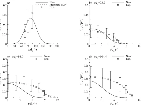
Figure III-2. BM-1atm flame. Temperature and mixture fraction distributions: a) axial distribution, b) to g) radial distributions at different heights. ... 58

Figure III-3. BM-1atm flame. Soot volume fraction distributions: a) axial distribution, b) to d) radial distributions at different heights. ... 59

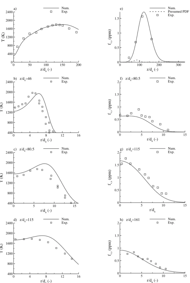
Figure III-4. BM-3atm flame. a) to d) radial distributions of temperature at different heights, e) axial distribution of soot volume fraction, f) to h) radial distributions of soot volume fraction at different heights. ... 61

Figure III-5. KH flame. a) axial distribution of temperature distributions, b) to d) radial distributions of temperature at different heights, e) axial distribution of soot volume fraction, f) to h) radial distributions of soot volume fraction at different heights. ... 62

Figure III-6. CJ flame. a) Axial distributions of mean and r.m.s values of temperature, b) axial distributions of mean and r.m.s. values of soot volume fraction, c) and d) radial distribution of mean and r.m.s. values of soot volume fraction at z/dn = 57 and z/dn = 84.5, respectively. ... 64

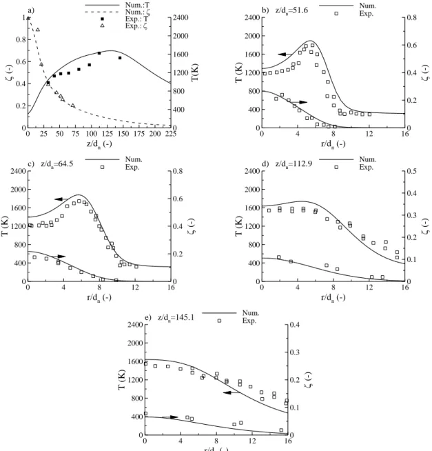
Figure III-7. YM flame. Temperature and mixture fraction distributions: a) axial distributions, b) to e) radial distributions at different heights. ... 65

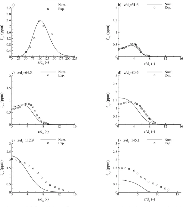
Figure III-8. YM flame. Soot volume fraction in the YM flame: a) axial distribution, b) to f) radial distributions at different heights. ... 66

Figure III-9. LTS flame. Radial distribution of mean and r.m.s values of temperature at different heights. . 67

Figure III-10. LTS flame. a) Axial evolution of mean and rms values of soot volume fraction, b) to f) radial distribution of mean soot volume fraction at different heights. ... 68

distance of 280 mm from the flame axis as a function of the height above the burner. ... 70 Figure III-12. NM flame. a) axial distributions of temperature and mole fraction of C2H2 and O2, b) to d) radial distributions of temperature at different heights, and e) and f) radial distributions of mole fraction of C2H2 and O2 at z/dn = 50 and z/dn = 150, respectively. ... 71

Figure III-13. NM flame. Soot mass concentration fraction: a) axial distribution, b) to f) radial distributions at different heights. ... 73 Figure III-14. WC3H8-OI21 and WC3H8-OI30 flames. a) Axial evolution of the equivalent soot volume fraction

and b) radiative wall heat flux. ... 74 Figure III-15. Wblend-OI21 and Wblend-OI30 flames. a) Axial evolution of the equivalent soot volume fraction

and b) radiative wall heat flux. ... 75 Figure III-16. Influence of approximate radiative models in the BM-3atm flame on: a) axial temperature and soot mass growth and oxidation rates, b) axial soot volume fraction, c) axial root mean square of temperature and soot volume fractions, and d) wall heat flux as a function of z/dn at z/dn = 25. ... 79

Figure III-17. Influence of approximate radiative models in the CJ flame on: a) axial temperature and soot mass growth and oxidation rates, b) axial soot volume fraction, c) axial root mean square of temperature and soot volume fractions, and d) wall heat flux as a function of z/dn at z/dn = 18.4. ... 80

Figure III-18. Influence of approximate radiative models in the WC3H8-OI30 flame on: a) axial temperature

and soot mass growth and oxidation rates, b) axial soot volume fraction, c) axial root mean square of temperature and soot volume fractions, and d) wall heat flux as a function of z/dn at z/dn = 25. ... 81

Figure III-19. a) Mean scalar dissipation rate field close to injection and b) shapes of PDF of the SDR for different values of σχ for a mean χ at 20 s-1 ... 85

Figure III-20. Axial profiles of a) mean temperature, b) rms temperature, c) mean soot volume fraction, d) rms soot volume fraction, e) radiative power and f) radiative wall flux for log-normal PDF simulation with σχ=1.36 and σχ=1 and Dirac PDF simulations ... 87

Figure IV-1. Evolution of the cross correlation between the soot volume fraction and temperature (solid line), and of the soot volume fraction (dashed line) a) along the flame axis, b) as a function of the radius at z=0.35 m... 91 Figure IV-2. Evolution of the equivalent soot volume fraction and radiative wall flux as a function of the height above the burner for the Full. and No Corr. computations ... 92 Figure IV-3. Fields of a) mean temperature (K) and b) mean soot volume fraction (ppm) for all five flames. ... 95 Figure IV-4. Axial profiles of a) mean soot fraction and b) r.m.s value of soot volume fraction for the ethylene flames. ... 96 Figure IV-5. Fields of a) soot emission term, b) fraction of the emission due to soot. ... 98 Figure IV-6. Fields of cross-correlation between soot volume fraction and temperature. ... 100 Figure IV-7. Structure of the flame in the region of significant soot emission along the axis for CH4-12000

flame (a) and C2H4-12000 flame (b). The vertical dashed line indicates the location of the stoichiometry.

... 101 Figure IV-8. Fields of the fraction of the soot emission due to the correlation between the soot absorption coefficient and the temperature ... 102 Figure IV-9. a) Axial evolution of the ratio between the soot absorption coefficient-blackbody intensity correlation and the soot emission term as a function of the height above the burner normalized by the flame length for the three-ethylene flames. b) Same as a) with the ratio between the soot absorption coefficient-blackbody intensity correlation and the soot emission term normalized by the turbulent intensity IT. .... 103

Figure IV-10. Axial profiles of the emission term computed with the four different closures (no TRIs, TRI1,

TRI2 and full TRI) for the five studied flames ... 106

Figure V-1. Axial evolution of the cross correlation between mixture fraction and enthalpy defect. a) as a function of the mixture fraction, b) as a function of the height above the burner. The evolutions of the mean enthalpy defect and the soot volume fraction are also plotted. The vertical continuous line in Fig. IV-1a represents the location of the mean stoichiometry. The vertical lines delimit the four regions. ... 110

Table III-1. Relative strengths and weaknesses of three PDF methods (from [153]) ... 46 Table III-2. Characteristics of the flames investigated. The characteristic residence time is defined as the time required to convect along the flame axis from the burner exit to the stoichiometric flame height. ... 54 Table III-3. Main numerical works concerning the flames investigated in the present study. N, SG and Ox denote nucleation, surface growth and oxidation, respectively. ... 56 Table III-4. Boundary conditions for the turbulent jet flames simulations ... 57 Table III-5. Comparison between predicted and measured values of fv,s,max, qR,w,max and χR. Rfv,s,max, RqR,w,max and

RχR represents the ratio of computed to measured values. ... 76

Table III-6. Influence of approximate radiative models on the peaks of temperature and soot volume fraction along the centerline. The error on the peak of temperature is calculated as ∆Tpeak=Tpeak,ref-Tpeak,approx and the

relative error on the peak of soot volume fraction and on the radiant fraction is computed as Rφ=φapprox/φref.

The complete radiative model is used as reference. ... 81 Table IV-1. Characteristics of the flames studied. ... 94 Table IV-2. Global radiative characteristics of the flames studied. ... 99 Table IV-3. Influence of different TRI closure on the soot emission. % indicate the relative effects (in %) defined as |<Es>noTRI,t-<Es>model,t|/<Es>noTRI,t ... 104

Chapter I Introduction

I.1 Context

Electricité de France (EDF), as an operator, is responsible for the safety of the nuclear plants and defines, in agreement with the regulation, the means and the organization implemented to ensure that its facilities do not present risks for the public and the environment.

Unwanted fires in nuclear plants is the most important risk for internal damage. Besides the safety of its staff and the operation of its facilities, EDF has an economical interest, related to the loss of material and immobilization, to reduce the fire risk by ensuring a high level of safety without using oversized firefighting means. The demonstration of the efficiency of fire safety with numerical models, due the improvement of knowledge and of computational resources, is increasing. The modeling tools developed by EDF R&D have been used for several years to answer questions relative to fire safety. Today, the two-zone code MAGIC is used as reference. It is based on the assumption of a stratification of the hot gases above the fresh gases and can provide rapid answers due to its low computational cost. Although this approach is efficient, it is not able to capture all the processes of the fire phenomena. In addition, it becomes less relevant in absence of stratification.

In order to circumvent these drawbacks, a CFD model of fire spread in nuclear plants is under development [43]. The present work is related to these developments. In particular, they will focus on soot production and radiative heat transfer and their coupling with turbulence.

Mass burning, flame spread and fire growth on hazardous scales are mainly driven by the radiative flux emitted by the gas combustion products, including soot, toward the environment and the condensed fuel surface, soot radiation being dominant in most

applications [44]. These fluxes provide the energy required to preheat the condensed fuel up to a sufficiently high temperature to vaporize it and, then, to release the gaseous fuel. This gaseous fuel is mixed with air and is ignited by the hot gas, ensuring the self-sustaining combustion process and/or the flame spread. Once the ignition phase processes are completed, these radiative fluxes provide the energy required to sustain the vaporization of the condensed phase on which the flame is established in order to supply it with gaseous fuel. In addition, because of the high levels of confinement encountered in building fires, the combustion takes place in relatively low-oxygenated conditions leading to partial or complete extinction of the flames. An accurate description of the evolution of fire in a confined environment requires, therefore, to correctly predict the concentrations of soot, the radiation of soot and combustion products, and to have a sufficiently detailed turbulent combustion model to describe local extinction/re-ignition processes.

I.2 Motivations

Fire dynamics are at the crossroads of several physical processes for which numerical modeling involve different strategies. As discussed previously, this includes fluid dynamics, heat and mass transfer including radiative transfer, combustion, soot production, thermal degradation of solid/liquid materials, multi-phase flow, and turbulence. In addition, most of these processes are strongly coupled mainly because of the turbulent nature of the flow [1,45]. This introduces closure problems for, on the one hand, the chemical reaction rates for both gaseous species and soot, and, on another hand, for the absorption and emission radiative terms [13]. These closure problems result from the non-linear nature of these terms. In the following, the closure problems due to the strong nonlinearity of the gaseous and soot production chemical source term will be denoted as Turbulence-Chemistry Interactions (TCI) and Turbulence Soot Production Interactions (TSI), respectively, and those due to the non-linearity of both absorption and emission radiative terms will be denoted as Turbulence-Radiation Interactions (TRI). TCI, TSI and Emission TRI depend on the turbulent fluctuations of local properties only (temperature, species concentrations) and can be evaluated by using a point one-time joint PDF of these quantities [19,46,47]. The simplest method, used commonly in fire simulation [1,48–51], is based on the conserved scalar approach and uses the uncorrelated approach to express the joint probability density function (PDF) of the

mixture fraction, scalar dissipation rate to measure the degree of departure from the equilibrium state, enthalpy defect to include radiative loss, and soot quantities [52]. The scalars involved in the PDF are assumed to be statically independent. The PDF of mixture fraction is often modelled as a clipped Gaussian or a 𝛽-PDF [19] whereas for the others scalars, including soot quantities, the corresponding PDF are modeled as Dirac delta functions centered on the mean value of the property [52]. This simplified approach is convenient on a numerical point of view but neglects the correlations between these quantities. The effects of these approximations are illustrated in Fig. I-1, which represents the axial profiles of temperature and soot volume fraction obtained by using the presumed PDF approach in a turbulent ethylene-air jet flame with a Reynolds of about 15,000 [18]. This figure shows clearly that the soot volume fraction is underestimated by more than one order of magnitude and, as a result, the temperature is overestimated. The sources of these discrepancies were explained by Moss and co-workers [52,53] and by Consalvi et al. [54]. They are due to the fact that the correlation between the mixture fraction and soot quantities, neglected in the present simulations, significantly affects the soot oxidation rate.

Figure I-1. Predicted and measured Left) soot volume fraction and Right) temperature in a turbulent ethylene-air jet flame by using a presumed PDF

method.



he same issue arises for the interactions between turbulence and soot emission radiative term which is a non-linear function of the soot volume fraction and temperature. The correlation between the soot volume fraction and the temperature, which is not taken

z (m) fv,s (p p m ) 0.2 0.4 0.6 0.8 1 0 0.1 0.2 0.3 0.4 0.5 0.6 0.7 0.8 0.9 1 Exp Presumed PDF z (m) T (K ) 0 0.2 0.4 0.6 0.8 1 400 800 1200 1600 2000 Exp_{Presumed PDF}

into account in the presumed-PDF approach, was found to be highly negative [55,56], which can have a significant effect on soot emission [48].

An alternative to the presumed-PDF approach is the transported PDF methods. They provide an elegant and effective resolution to the closure problems described previously. PDF methods are discussed in details in the books by Pope [57] and Fox [14]. A comprehensive review can be found in [13], and a perspective on recent advances and trends can be found in [47]. In addition, the modeling of extinction/re-ignition processes encountered in under-ventilated fires require to use a direct coupling between the chemical kinetic and the flow, and TCI are handled in an exact manner by transported PDF methods [12,13].

I.3 Objectives of the thesis

The main objective of the present thesis is to develop, implement and validate a transported PDF method, in conjunction with well-established sub-models for turbulent combustion, soot production and radiative transfer. The developments are performed in a RANS framework and by using a flamelet combustion model. These latter choices are not limitations of the model since transported PDF methods can be also used as sub-filter-scale models for large-eddy simulation (filtered density function methods) and are designed to model exactly chemical source terms. A semi-empirical acetylene-benzene-based two equations model for soot production [6], and a Wide-Band Correlated-k (WBCK) model for the gas radiative properties [8] will be considered.

The second objective of the thesis to provide a better understanding of soot emission TRI which can be modeled exactly using the transported PDF method. The effects of the correlation between the mixture fraction and enthalpy defect, which are usually disregarded when presumed PDF methods are used, will also be investigated.

I.4 Bibliographic survey

I.4.1 Physical processes governing fire dynamics

This section will describe the main processes involved in the development of fires. First, the combustion and heat transfer regimes encountered will be discussed as well as

the main steps observed in the development of a fire in a compartment. Finally, the specificity of under-ventilated fires will be discussed.

I.4.1.1 Flow, combustion and heat transfer regimes of fires

Combustion studies are usually divided into three categories [19]: premixed flames for which the reactants are mixed before ignition, diffusion flames for which the reactants are brought separately to the reaction zone, and partially premixed flames for which a fraction of injected reactants mixes before reaching the reaction zone. Flames encountered in well-ventilated fires usually burn in the diffusion flame regime.

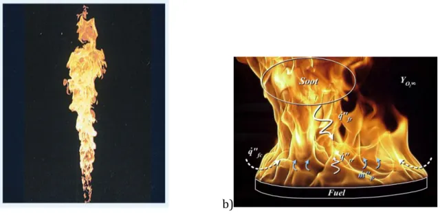
In diffusion flames, the reactants are injected separately and diffuse to the reaction zone. The schematic structure of a diffusion flame is given in Fig. I-2. A key characteristic of diffusion flames is the fact that they do not propagate, the mixture being either too rich (on the fuel side) or too lean (on the oxidizer side) for the combustion zone to spread. Diffusion flames are therefore safer to operate in industrial processes than premixed flames. Mixing is the key issue in diffusion flames dynamics. The chemical reaction will only take place in a limited region where the reactants are mixed close to the stoichiometric proportions. The lack of propagation also makes diffusion flames more sensitive to velocity fluctuations and, therefore, to turbulence.

One of the most common kind of diffusion flame is the jet flame, for which an instantaneous picture is given in Fig. I-3a. Gaseous fuel is injected with a high velocity in an oxidizer co-flow or in atmospheric air, and ignited. Jet flames are often used as validation cases for turbulent combustion model. The high injection velocity implies that the production of turbulence due to buoyancy can usually be neglected in the case of laboratory-scale turbulent jet flames.

a) b)

Figure I-3. Diffusion flames structure: a) Jet diffusion flame, and b) Pool fire.

Unwanted fires mostly evolve in the buoyancy-driven regime (see Fig. I-3b). The Froude number, 𝐹𝑟 = 𝑢_𝑖𝑛𝑗2 _{⁄𝑔𝐿, is typically in the range 10-6-10-2. In the previous}

expression 𝑢_𝑖𝑛𝑗 is a typical fuel injection velocity, 𝑔 is the gravitational acceleration and 𝐿 is a characteristic length, typically the flame length or the diameter of the burner in the present example. The pool fire scenario, described in Fig. I-3b, represents a simplified version of fires that occur in practice. In this case, the condensed phase (liquid or solid) is transformed into gaseous volatiles either by pyrolysis (degradation of solid or heavy liquid by convective or radiative heat transfer) or by vaporization (for light liquids). The gasification processes occur due to the influence of the convective and radiative fluxes transferred by the flame. Gaseous fuel is then transported by convection/diffusion to the reaction zone where they mix with the oxygen of air to react, which makes this process

self-sustained. For well-ventilated medium, the chemistry can generally be assumed to be fast as compared to the mixing which allows simplifying the description of the gas phase combustion.

The dominant mode of heat transfer between the flame and the condensed material depends on the size of the pool: at small-scale the heat transfer is dominated by convection whereas for pool fires with diameters greater than a meter thermal radiation prevails. Let us consider the energy balance at the surface of a liquid fuel:

𝑚̇_𝑝𝑦𝑟" 𝐿_𝑣 = 𝑞_{𝑓𝑙,𝑟𝑎𝑑}+ 𝑞_{𝑓𝑙,𝑐𝑜𝑛𝑣}− 𝑞_𝑟𝑟− 𝑞_{𝑐𝑜𝑛𝑑} (I-1) where 𝑚̇_𝑝𝑦𝑟" _{is the pyrolysis mass flow rate. 𝑞}

𝑓𝑙,𝑟𝑎𝑑, 𝑞𝑓𝑙,𝑐𝑜𝑛𝑣, 𝑞𝑟𝑟 and 𝑞𝑐𝑜𝑛𝑑 represent the

heat flux transferred by the flame by radiation and convection, the heat flux emitted by the fuel surface and the heat flux transferred in the material by conduction. 𝐿_𝑣 is the latent heat of vaporization. This expression can be simplified for large-scale fires on the basis of the analysis carried out previously:

𝑚̇_𝑝𝑦𝑟" _𝐿

𝑣 ≅ 𝑞𝑓𝑙,𝑟𝑎𝑑 (I-2)

On the other hand, the heat release rate can be written as:

𝑄̇ = 𝑚̇𝑝𝑦𝑟" 𝑆𝑏𝑢𝑟𝑛∆ℎ𝑐 (I-3)

where 𝑆𝑏𝑢𝑟𝑛 represents the pyrolysing surface and ∆ℎ𝑐 is the heat of combustion. As a

consequence, it appears that for large-scale fires, the radiative flux transferred from the flame toward the condensed material plays a crucial role in the determination of the heat release rate. Gaseous combustion products (CO2, H2O, CO, and some hydrocarbons) and

soot are responsible for the radiative heat flux from the flame. Gaseous species emit radiation on some discrete bands, whereas the radiation from soot is continuous, covering the entire thermal spectrum. The contribution of soot depends widely on the combustible. Nevertheless, in “real” fires, their contribution usually prevails [44].

In addition, flames encountered in fires are turbulent. The influence of turbulent motions on diffusion flames is important on several levels. First, for any combustion problem, turbulent-related phenomena include flame-generated vorticity, viscous effects, and stretching [19]. Second, diffusion flames do not propagate and have little impact on

flow dynamics. Therefore, they are much more sensitive to turbulent motions than premixed flames (especially regarding stretching and quenching). Furthermore, buoyancy, natural convection and entrainment effects, as well as molecular diffusion can all be affected by turbulence [19].

I.4.1.2 Development of a confined fire

Figure I-4. Heat release rate during the evolution of a fire.

The development of a confined fire can be divided into the following five major stages [58,59], illustrated on Fig. I-4:

Ignition: Ignition can be considered as a process that produces an exothermic

reaction characterized by an increase in temperature greatly above the ambient. It can occur either by piloted ignition (by flaming match, spark, or other pilot source) or by spontaneous ignition (through accumulation of heat in the fuel). The accompanying combustion process can be either flaming combustion or smoldering combustion.

Growth: Following ignition, the fire may grow at a slow or a fast rate, depending on

the type of combustion, the type of fuel, interaction with the surroundings, and access to oxygen. The fire can be described in terms of the rate of energy released and the production of combustion gases. A smoldering fire can produce hazardous amounts of

toxic gases while the energy release rate may be relatively low. The growth period of such a fire may be very long, and it may die out before subsequent stages are reached. The growth stage can also occur very rapidly, especially with flaming combustion, where the fuel is flammable enough to allow rapid flame spread over its surface, where heat flux from the first burning fuel package is sufficient to ignite adjacent fuel packages, and where sufficient oxygen and fuel are available for rapid fire growth. Fires with sufficient oxygen available for combustion are said to be fuel-controlled.

Flashover: Flashover is the transition from the growth period to the fully developed

stage in fire development. In fire safety engineering, the word is used as the demarcation point between two stages of a compartment fire, i.e., pre-flashover and post-flashover. Flashover is not a precise term: several variations in definition can be found in the literature. The criteria given usually demand that the temperature in the compartment has reached 500–600°C, or that the radiation to the floor of the compartment is 15 to 20 kW/m2_{, or that flames appear from the enclosure openings. These occurrences may all be}

due to different mechanisms resulting from the fuel properties, fuel orientation, fuel position, enclosure geometry, and conditions in the upper layer. Flashover cannot be said to be a mechanism, but rather a phenomenon associated with a thermal instability.

Fully developed fire: At this stage the energy released in the enclosure is at its

greatest and is very often limited by the availability of oxygen. This is called ventilation-controlled burning (as opposed to fuel-ventilation-controlled burning), since the oxygen needed for the combustion is assumed to enter through the openings. In ventilation-controlled fires, unburnt gases can collect at the ceiling level, and as these gases leave through the openings they burn, causing flames to stick out through the openings. The average gas temperature in the enclosure during this stage is often very high, in the range of 700 to 1200°C.

Decay: As the fuel becomes consumed, the energy release rate diminishes and thus

the average gas temperature in the compartment declines. At this point, the fire may go from ventilation-controlled to fuel controlled.

As can be seen from the steps outlined above, fire dynamics are at the crossroads of several different physical processes. It involves fluid dynamics, combustion, hydrocarbon

chemistry, radiative transfer, thermal degradation of solid and liquid fuels, multi-phase flow, production of soot, and all these phenomena are coupled (see Fig. I-5).

Figure I-5. Schematic of the processes involved in a compartment fire [58]

I.4.1.3 Fire in confined compartments

The specificity of fires in nuclear plants is that they occur with a high level of confinement, leading to conditions for combustion generally different from those encountered in well-ventilated fires. Air feeding the flame becomes rapidly vitiated, which leads to incomplete combustion. Gaseous combustibles, soot, carbon monoxide and other pollutants then escape from the fire and are released in the surroundings. This can lead to extremely dangerous hazards, especially if the gaseous combustible mixes with air and encounter points with a sufficiently high temperature to ignite this mixture.

The vitiation of air should lead to a reduction in flame temperature, implying a decrease in the radiative heat transfers and then pyrolysis mass flow rates. These trends appear clearly in the evolution of the pyrolysis mass flow rate measured during the PRISME experiments performed at the IRSN for different levels of vitiation [60]. On the other hand, the high temperature of the enclosure walls surrounding the fire should produce a supplementary source of heating for the pyrolysis and growth processes. The

soot production should be also considerably affected [61]: on one hand the decrease in flame temperature should reduce the soot formation rates, leading to lower soot concentrations. On the other hand, decreasing the oxidation process, should lead to higher soot concentration. As a consequence, it is difficult to determine a priori how the total amount of soot will evolve when the oxygen concentration will decrease.

I.4.2 Soot production

Soot is a mass of impure carbon particles resulting from the incomplete combustion of hydrocarbons. Soot is not a uniquely defined chemical substance in that it contains mostly carbon, with up to 10% (mol) of hydrogen. The atomic C/H ratio is about 8 to 1. The mass density of soot is about 2 g/cm3_{. Electron microscopy studies show that a soot}

particle often consists of chain-like aggregates of nearly spherical particles. These spherical particles, called the primary particles, may contain between 105 _{to 10}6 _carbon

atoms, and usually have diameters between 20 to 50 nm [62].

Figure I-6. Characteristic time scales for the chemical and physical processes (From Mass and Pope [63])

The modeling of soot production introduces two difficulties as compared to the modeling of gaseous reactants:

- The first difficulty can be analyzed from Fig. I-6 which shows the characteristic time scales for the different physical and chemical processes. When the chemistry is sufficiently fast, i.e. characteristic times for chemical processes are much lower than those of the flow, the chemical reactions attain a quasi-steady state and adjust with short relation times to local flow conditions. Consequently, the chemistry and the mixing processes can be decoupled. This is the basis concept of the flamelet [3]. State relationships for the different reactive scalars can then be generated, such as the temperature or the species mass fraction, as a function of a reduced number of parameters describing the local flow conditions (mixture fraction, scalar dissipation rate, radiative loss). Figure I-6 shows that the chemistry associated to soot, and more generally to pollutants, is slow. As a consequence, the simplifications described previously cannot be rigorously applied.

- The second difficulty comes from the fact that, contrary to NO and other pollutants, soot acts on the flow through the radiative losses that it produces. As a consequence, the formation of soot cannot be considered at posteriori, i.e. once the flow-field has been predicted. This implies that radiative heat transfer must be taken into account in an accurate manner, soot formation/oxidation processes being sensitive to temperature. The effects of the coupling between soot formation and radiative heat transfer are significant in both laminar and turbulent coflow diffusion flames [64–67].

I.4.2.1 Physical mechanisms

Soot formation and dynamics in combustion systems are usually decomposed into four different processes: nucleation, surface reaction growth, oxidation and coagulation. Nucleation and coagulation control the number of primary particles, whereas surface reactions (surface growth and oxidation) control the carbon mass accumulated in soot.

I.4.2.1.1 Nucleation

The first step of soot formation is the nucleation. The first soot particles appear from PAH (Polycyclic Aromatic Hydrocarbons), which are formed from species like acetylene and benzene, produced by the degradation of hydrocarbon. Nucleation can itself be divided into 3 sub-processes [68]: initial PAH formation (formation of the first aromatic