Analytics for Hotels: Demand Prediction and Decision
Optimization
by
Rui Sun
B.Eng. Automation, Tsinghua University, 2014
Submitted to the Department of Civil and Environmental Engineering and the Department of Electrical Engineering and Computer Science
in partial fulfillment of the requirements for the degrees of Master of Science in Transportation
and
Master of Science in Electrical Engineering and Computer Science at the
MASSACHUSETTS INSTITUTE OF TECHNOLOGY
June 2017
Massachusetts Institute of Technology 2017. All rights reserved.
Signature redacted
A u th o r . .. .. ... . ... ... ... .. ... .. ... Department of Civil and Environmental Engineering Department of Electrical Engineering and Computer Science
Certified by ...
Signature redacted
I/ V
May 19, 2017
David Simchi-Levi Professor of Engineering Systems, Institute for Data, Systems, and Society /hesis Supervisor Certified by...
Joan and Irwin
Accepted by... Accepted by ... MASbUU~ I NS) I) IT I E OF TECHNOLOGY
JUN 14 2017
...
re d acte d
Vincent Chan Jacobs Professor of El ical Engineerin and Computer Science171 /r- IfThesis Reader
Signature redacted
Thesis.ReaderJesse Kroll Professor of Civil and Environmental Engineering
A Chair,, Graduate Program Committee
...
CISignature redacted
LU
0
/
C Leslie A. KolodziejskiAnalytics for Hotels: Demand Prediction and Decision
Optimization
by
Rui Sun
Submitted to the Department of Civil and Environmental Engineering and the Department of Electrical Engineering and Computer Science
on May 19, 2017, in partial fulfillment of the requirements for the degrees of
Master of Science in Transportation and
Master of Science in Electrical Engineering and Computer Science
Abstract
The thesis presents the work with a hotel company, as an example of how machine learning techniques can be applied to improve demand predictions and help a hotel property to make better decisions on its pricing and capacity allocation strategies. To solve the decision optimization problem, we first build a random forest model to predict demand under given prices, and then plug the predictions into a mixed integer program to optimize the prices and capacity allocation decisions. We present in the numerical results that our demand forecast model can provide accurate demand predictions, and with optimized decisions, the hotel is able to obtain a significant increase in revenue compared to its historical policies.
Thesis Supervisor: David Simchi-Levi
Title: Professor of Engineering Systems, Institute for Data, Systems, and Society
Thesis Reader: Vincent Chan
Title: Joan and Irwin Jacobs Professor of Electrical Engineering and Computer Sci-ence
Acknowledgments
Firstly, I would like to express my sincere gratitude to my advisor Prof. David Simchi-Levi for his continuous support of my research, for his patience and motivation. His thoughtful insights, broad perspective, and research passion have been and will continue to be my sources of inspiration. Without his guidance and encouragement, this thesis would not have been possible.
I would also like to thank my thesis co-advisor Professor Vincent Chan, for his
valuable advices and comments, and the challenging questions he has proposed, which have incented me to widen my research from various perspectives.
I would like to thank my project partners from Starwood for sharing their expertise
and experiences, and for providing valuable feedback throughout this research. It has been a great pleasure to work with them.
I would like to thank my research collaborator Eduardo, Candela Garza who has
been very resourceful in research discussions. His commitment towards the project was a significant influence in shaping many of the concepts presented in this thesis.
I would like to thank my fellow labmates and my friends at MIT, for the stim-ulating discussions, for the sleepless nights we have worked together and for all the fun we have had together. Their friendship and companion have enriched my life at MIT.
Last but not the least, I owe my deepest gratitude to my parents for their uncon-ditional and unparalleled love. This thesis is dedicated to them.
Contents
1 Introduction 13 1.1 Literature Review . . . . 17 2 Problem Formulation 21 2.1 D ata . . . . 21 2.2 Demand Variables . . . . 22 2.3 Decision Variables . . . . 24 3 Demand Prediction 27 3.1 Preprocessing . . . . 27 3.2 Prediction Model . . . . 30 3.3 Numerical Results . . . . 33 3.4 Discussion . . . . 37 4 Decision Optimization 41 4.1 Markov Decision Framework . . . . 414.1.1 MDP Simplification . . . . 44
4.2 Mixed Integer Programming . . . . 47
4.2.1 Basic Formulation . . . . 47
4.2.2 Model Enhancement . . . . 50
4.2.3 Equivalence to a linear program . . . . 53
4.3 Numerical Results . . . . 54
4.5 Im plem entation . . . . .. .. ... . . .. . . . . 5 Conclusions and Future Research
A Demand Prediction
62 65 67
List of Figures
1-1 Histogram of the occupancy distribution of one hotel property . . . . 14
1-2 The average quantity of bookings and prices in each booking window for two major customer segments . . . . 15
2-1 Illustration of arrival dates, stay dates and booking windows . . . . . 22
2-2 Data sum m ary . . . . 23
2-3 Description of the demand variables defined in different periods . . . 24
2-4 An illustrative example on using pricing decisions only . . . . 26
3-1 The input and output variables for our demand prediction model . 31 3-2 Illustrative example of a regression tree . . . . 32
3-3 Distribution of prediction errors in all booking windows . . . . 36
3-4 Variable importance analysis for our prediction models . . . . 37
4-1 A table explanation for formulation (PO) . . . . 48
4-2 List of revenue metrics . . . . 55
4-3 Comparison of different revenue metrics . . . . 56
4-4 Revenue comparisons . . . . 57
4-5 Distribution of the average price change in each booking window . . . 58
4-6 Distribution of pricing decisions . . . . 59
4-7 Distribution of revenue improvements against capacity leftovers . . . 60
4-8 Comparison on capacity leftovers between optimal decisions and his-torical decisions . . . . 60
A-1 Distribution of mean percentage errors in each booking window for
m odel R F2 . . . . 67 A-2 Gini variable importance analysis for our prediction models . . . . 68
List of Tables
3.1 Details on the aggregation of booking windows and the average of
number of bookings in each booking window . . . . 29
3.2 Performance metrics . . . . 34
3.3 Dataset comparison for different models . . . . 35
The thesis presents the work with a hotel company, as an example of how machine learning techniques can be applied to improve demand predictions and help a hotel property to make better decisions on its pricing and capacity allocation strategies. To solve the decision optimization problem, we first build a random forest model to predict demand under given prices, and then plug the predictions into a mixed integer program to optimize the prices and capacity allocation decisions. We present in the numerical results that our demand forecast model can provide accurate demand predictions, and with optimized decisions, the hotel is able to obtain a significant increase in revenue compared to its historical policies.
Chapter 1
Introduction
The thesis presents the work with a hotel company, as an example of how machine learning techniques can be applied to improve demand predictions and help a hotel property to make better decisions on its pricing and capacity allocation strategies. With the objective of maximizing revenue, one of the challenging problems faced by hotels is to decide what prices to charge and how many rooms to allocate to each booking period. The mechanism behind this is simple: since customers who arrive at different time windows tend to have different price sensitivities, revenue could be maximized by using differentiating pricing policies. It is generally considered that customers who make their bookings late would have a higher willingness-to-pay. Therefore, hotels can increase revenue by charging higher prices as the booking period gets closer to the stay date and saving rooms from the total capacity for late-booking customers.
The key to make good pricing and capacity control decisions is to predict cus-tomer's demand precisely, especially demand of the late booking periods. If the number of late bookings is under-predicted, the hotel would allocate more rooms to early periods or even decrease prices in late periods to attract more customers; if the number of late bookings is over-predicted, the strategy would be to save rooms for late periods and increase prices to exclude customers with low willingness-to-pay. In either case, imprecise demand predictions would lead to poor decisions and prevent the hotel from earning more profits.
~'00,) 600o 50% 40% 20% 10%200/0 10% -- ---
I
0.5- [0.5.0.6) [0.6,0.7) [0.7,0.8) [0.80.9) [0.91.0) 1.0-Occupancy LevelsFigure 1-1: Histogram of the occupancy distribution of one hotel property
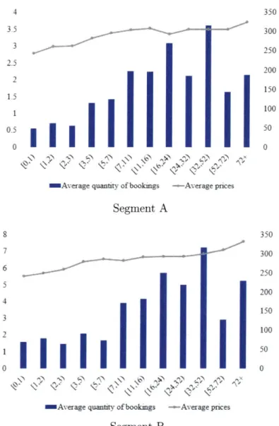
To obtain accurate demand forecast is also the main focus of our work, as we find that the hotel company's current forecast model has lead to inappropriate decisions as shown in Fig. 1-1 and Fig. 1-2. The observation is made in two steps. First we present in Fig. 1-1 a histogram of the occupancy distribution of a specific hotel property, where occupancy is the percentage of rooms out of the total capacity that have been booked until the final day1. The figure shows that in 80% of the days, the occupancy is greater than 90%, which indicates demand for the hotel is always on a high level. Next in 1-2, we present the analysis for the hotel's historical demand and booking prices from its major customer segments. In the plot, x-axis represents the time windows, which is defined as the number of days prior to the stay day of a customer. (For example, [3,5) means the customer books his room 3 or 4 days before his planning stay date.) The left y-axis represents the average quantities of bookings in each booking window and the right y-axis represents the average prices. We can see that as the booking window gets closer to the stay dates, the average price decreases, so does the number of bookings, and this implies low prices were employed by the hotel to fill in the capacity in the late periods. If we combine this observation with the high demand level we observe in Fig. 1-1, we can conclude that the historical policies have failed to protect the capacity for late-booking customers and the high willingness-to-pays, thus denting the revenue that could otherwise be earned by a better policy. On
'In some cases where a customer leaves earlier, a hotel room could serve for two different bookings on the same day, and thus occupancy could be greater than 1.
4 350 35 300 3 250 2.5 200 2 10 1 100) 0.5 50 0 0
Average quantity of bookings - Aver-age pnce~s
Segment A 8 7 6 5 4 3 2 0
Average quantity of bookings -- Average prces
Segment B 350 300 250 200 150 100 50 0
Figure 1-2: The average quantity of bookings and prices in each booking window for two major customer segments
the other hand, decreasing prices in the long term might inspire customers to book late and stimulate the cancellations of early bookings, introducing more problems into policy designs. These observations suggest the room for improvement in terms of revenue maximization and motivates the development of a precise demand prediction model as well as associated decision support tools to improve the hotel's pricing and capacity allocation decisions.
Our approach to solve the problem includes two stages: 1) we begin with building a demand prediction model to forecast the number of bookings in each time period; 2) we plug the prediction results into an optimization model to find the optimal
pricing and capacity control decisions that maximize revenue. The main challenge in predicting demand is how to model its relationship with price. For customers booking in different time periods have different price sensitivities, a uniform demand-price function for all booking periods is likely to fit badly to the data. There also exist such variances of price sensitivities in different market segments, room classes and stay dates. To address the challenge, we build our forecast model based on random forest, which is a generalized and nonparametric tree model, established as one of the essential machine learning techniques. Random forest can handle categorical variables together with numerical variables and differentiate variant categories by itself. Moreover, it can return the importance of each categorical variable; and lastly, a random forest reduces the prediction variance of a single tree by aggregating the prediction results of all its subtrees. These advantages make random forest a good model in terms of simplicity, interpretability and predictability.
We then formulate an optimization model to optimize price and capacity alloca-tion decisions, taking demand predicalloca-tions under variant prices generated in the first stage as inputs. In this stage, the biggest challenge is how to solve the problem ef-ficiently. Since revenue is the product of price and demand, and the latter depends on our capacity allocation decisions, nonlinear terms hence appear in the objective function. To simply the model, we first develop an equivalent mixed integer formu-lation using the binary linearity property of price indicators, and then prove that it can be equivalently solved as a linear optimization problem. This observation enables us to solve a complicated optimization problem with efficient algorithms designed for linear optimization models. Furthermore, we enhance the model to incorporate room hierarchy constraints and fixed price constraints. Results from numerical experiments estimate that we can obtain a revenue increase around 14.5% for a specific hotel prop-erty. Our solutions also provide the hotel company with meaningful decision-making suggestions.
The thesis is structured as follows: in the remainder of this section, we provide a literature review on related researches and state the main contributions of our work. In Chapter 2, we introduce in detail the basic settings of the problem and the data
we are provided. The next two chapters focus on our methodologies: in Chapter
3, we explain how to build a random forest model to predict demand, and provide
some numerical results to show its prediction accuracy; in Chapter 4 we present our formulation for the decision optimization problem, and show the numerical results produced by our optimal solutions. Finally, Chapter 5 concludes the thesis with a summary of our main results and potential future research scopes.
1.1
Literature Review
We are solving a problem that optimizes the pricing and capacity allocation decisions of a hotel property, a classical problem in the revenue management (RM) field. To the best of our knowledge, the very beginning of revenue management is built on the work by Littlewood in 1970s
[19]
where he studies a seat allocation problem motivatedby the airline industry and proposes a marginal seat revenue principle for a two-price
single-leg flight model, which is later known as the Littlewood's Rule. Many yield control methods have then been developed subsequently focusing on expanding the theory to multiple time periods, multiple fare classes and networks with multiple flights. The problem has been well-studied with dynamic programming methods as well as heuristic algorithms. A review of the related topics and their main results can be found in [21] and [25].
One common assumption in the traditional resource allocation literature is that the underlying distributions of demand are known as a priori, which might not be the case for practical problems. This motivates another stream of research in revenue management that focuses on pricing, demand learning, and also joint pricing and inventory control problems; see [11] for a recent survey. Specifically, some works prefer parametric demand models for their good statistical tractabilities: for example,
[16] studies a Bayesian pricing policy with binary prior distribution;
[9]
studies a general choice model with maximum likelihood estimations; [17] studies a linear model for multiple products. While some other works focus on non-parametric methods: for example, [18] proposes a bisection search algorithm for problems with inventoryconstraints; [27] designs an algorithm with iteratively shrinking learning intervals;
[10] uses linear approximations to solve a joint pricing inventory control problem
with lost sales and censored demand. To sum up, the mutual challenge for the work with the learning flavors is to balance the trade-off between learning (explorations) and earning (exploitations), and they all emphasize on the development of practical policies that have provably good performance although are not necessarily optimal.
In fact, most of the demand learning algorithms in revenue management are de-signed for problems where there are typically long sales horizons, high demand vol-umes and identically distributed demand variables, such as the pricing problems in online selling and financial services. While for traditional industries, like airlines and hotels, the effective booking horizon is short, and the demand volume is relatively small, and additionally, demand patterns in different booking periods and differ-ent days are not iddiffer-entical. In these environmdiffer-ents, applying online demand learning algorithms would be very expensive. Therefore, in our problem, we abandon the on-line learning structure and instead develop a prediction-optimization framework that works in an offline manner. We borrow the idea from the work done in [14] which develops a pricing device for an online retailer. The work employs a machine learning tool, regression tree, to forecast demand and then formulates an integer programming model to optimize prices. This framework makes it possible to separate prediction and optimization. Moreover, it can be easily implemented in practice.
Another stream of revenue management research that becomes popular nowadays is to use approximate dynamic programming approaches to solve a Markov decision model. The Markov decision framework is a powerful modeling tool that can provide closed-loop optimal control strategies, but it tends to suffer from the curse of dimen-sionality as the scale of the problem grows. Approximate dynamic programming is proposed to address the dimensionality issue by approximating state-cost values with parametric functions. The books
[3] [4] 122]
are referred for details on the related the-ories and variant algorithms to solve an approximate model. In terms of applications in the revenue management field,[131
[29][301
have provided some good examples on applying approximate methods to solve network revenue management problems.We will also introduce later in the thesis how to formulate our optimization problem into a Markov decision model and briefly discuss some approximate methods we can possibly implement without displaying the mathematical details.
The main contributions of our work in this thesis are as follows. Firstly, we build a demand forecast model with random forest, which provides a practical example for applying machine learning techniques to estimate demand in general revenue man-agement problems. Secondly, we provide an integer programming formulation to find the optimal pricing and capacity control decisions for a hotel property and prove its equivalence to its linear relaxation model. Additionally, we take into account room hierarchy constraints and fixed price constraints in the optimization of decisions. All these results can be considered as contributing to the pricing and resource allocation literature. Lastly, our numerical results are based on real-world data, so they can provide hotel companies with meaningful and critical insights on how to build good demand forecast models as well as make better pricing decisions in practice.
Chapter 2
Problem Formulation
In this chapter, we will present the basic settings of our problem formulation. We
begin with a description of the data, and then move on to the assumptions we have made in defining the demand and decision variables. Some discussions on the related approaches as well as the limits we might have in tackling the problem will also be covered.
2.1
Data
In the problem, we are provided with a specific hotel property owned by the com-pany, which has multiple room classes and market segments. Market segments are classifications of customers, and each segment stands for a specific customer feature or a pricing constraint. In the data there are in total 17 market segments and they are all priced differently. In terms of pricing constraints, there exist price-affected market segments where customers are subject to price changes, and contract-related market segments where customers have contract deals with the hotel company and their booking prices are fixed beforehand. As for room classes, there are five room classes for the given property, and they are mostly defined by the features of a room. We are also provided with a room class hierarchy which allows customers to be up-graded from a lower room class to a higher room class when the lower class is out of capacity.
Booking window Arrival date 1
Arrival date 2
Arrival date 3 W
I I
Stay date 1 Stay date 2
Figure 2-1: Illustration of arrival dates, stay dates and booking windows
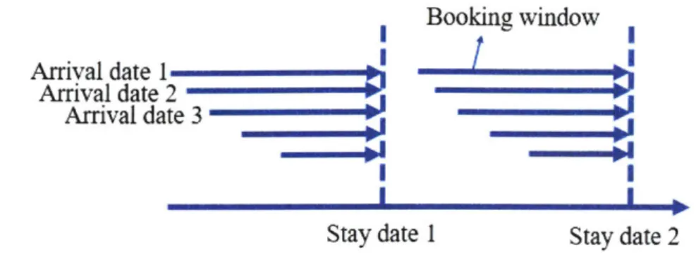
The data covers the booking history of a year, and for each stay date of the year, it includes the price and the number of bookings for each booking window, market segment and room class. Here, the number of bookings are counted by stay dates rather than arrival dates. In fact, a stay date is the date that a customer plans to stay at the hotel, while an arrival date refers to the date that a customer makes his or her booking, i.e. the date when the booking arrives. The days between an arrival date and a stay date is called a booking window. Fig. 2-1 shows an example illustrating the definitions of these terms. For a summary of the data, see Fig. 2-2. In the following, we will explain the definitions of demand and decision variables in our problem.
2.2
Demand Variables
The demand variables in our problem stand for the quantity of bookings, and in our model, the number of bookings is counted by the stay dates. Such a treatment has the following two advantages: first, we can easily distinguish early bookings and late bookings, since stay-date demand directly defines the booking windows; second, we do not need to worry about the seasonality factors, because the booking windows for different stay dates are independent. While the shortcoming of stay-date demand is also evident. It tends to ignore the interrelations of demand on consecutive arrival dates: in the case where a customer books five nights in a row, the booking for each stay date is counted individually. Nevertheless, in practice, prices are decided individually for different stay dates, so in terms of the alignment with decisions,
Room Class Booking Records
- Room hierarchy * Stay date
- Room capacity Booking window Market segment Market Segment * Room class
- Contract-related - Room rate (price)
- Price-affected - Quantity of booking (demand)
Figure 2-2: Data summary
modeling demand by the stay dates is a more convenient way.
One concern in dealing with demand is the dependency among the number of
bookings in different booking windows, market segments and room classes. Consider
the case where a customer saw the price but did not book in the first place, he or she
might choose to wait and make his or her booking in later periods. It is also possible
that the customer would switch from a market segment with refundable policies to
another market segment that does not offer any refunds, or even upgrade the room
class from a standard room to a luxury suite. In these situations, demands in different
units are interrelated, and the number of bookings in a unit is likely to depend on
the prices of other units.
To capture the demand interdependence is a challenging problem. It would
in-troduce extra explainable variables and make the prediction model complicated. In
the current problem setting, we simply assume that demand in different units are
independent, i.e. the number of bookings in one unit is not affected by the prices
of other booking units. In fact, most of the market segments in our problem is
de-signed by the hotel company in an independent manner: one market segment could be
only for customers who own membership accounts, and another might be exclusively
for employees from companies that have partnership agreements. Similarly, different
room classes also have distinct features. These designs of market segments and room
classes justify our assumption to some extent.
'For convenience of discussion, in this and the following chapters, we adopt the term booking unit, or simply unit, to represent a unique combination of booking window, market segment and room class.
Unconstrained Demand
Total arrivals of potential bookings
- - - - - I
-----j ----------
-Price-constrained Demand - Inventory-constrained Demand
The number of bookings The number of bookings after adjusted by prices finally accepted by the system
Figure 2-3: Description of the demand variables defined in different periods
The last thing worth discussion is the estimation of lost sales. As shown in Fig.
2-3. the final number of bookings we have in the booking system is adjusted through
two steps: in the first step, the unconstrained demand, as an estimation of customers' total arrivals, is adjusted by prices and then produces the price-constrained demand; in the second step, some of the demand might be rejected due to capacity allocation decisions and the accepted part becomes the inventory-constrained demand. In this process, the true number of bookings under given prices might be truncated by the capacity controls. So it is necessary to restore the rejected part of demand before we build a prediction model. This reverse engineering procedure is also known as the estimation of lost sales, an issue faced by almost all retailers. There has been a lot of work done under this topic: an overview of the common methods is provided in [25j and some extensions of the ideas can be found in 1141
[20]
[26J. While in our problem,we have no access to the historical capacity control decisions. It is thus infeasible to get an accurate estimation or to apply any statistical methods. Instead, we use a straightforward method to remove the data that might be truncated. The details on our method will be discussed later in Chapter 3.
2.3
Decision Variables
The objective of our problem is to maximize revenue with special constraints on room hierarchy and contract-related market segments, and there exist two types of decision
variables: prices and capacity allocations. Capacity here stands for the number of rooms from different room classes. Recall that our approach for the problem is two-fold: we first need to develop an accurate demand prediction model to forecast the number of bookings in each unit; then with the prediction results, we optimize the pricing and capacity allocation decisions. Therefore, our decision variables should be defined on the same unit level as the demand variables. Moreover, we assume that decisions for each stay date are optimized individually, and we are not considering the dependence in the bookings for consecutive nights.
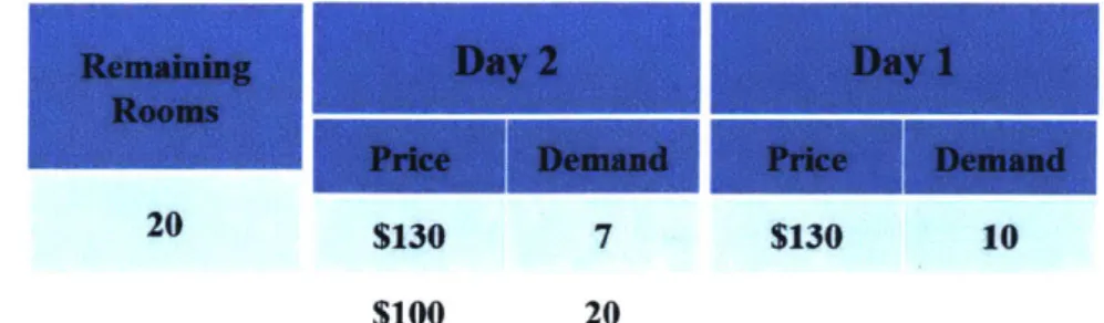
An interesting question to discuss is whether or not we need capacity allocation decisions in our optimization models. It seems that capacity controls can be translated into equivalent pricing decisions: when demand is lower than the allocated capacity, allocation decisions are not in effect; and when demand is higher than the assigned capacity, we can reject extra bookings by charging a super high (close to infinity) price. In fact, removing capacity allocation decisions could significantly simply our formulations and optimization algorithms, however, the following counterexample shows that we might fail to find the true optimal decisions without capacity controls. Consider the case where there are 20 available rooms and we are 2 days before the stay date. In the first booking period (day 2), assume demand is 20 at price $100 and 7 at price $130; while in the second booking period (day 1), demand is 10 at price $130. For both booking periods, it is assumed that we can set price as infinity to obtain zero bookings. The optimal policy here is to allocate 10 rooms to day 2 at price $130, 10 rooms to day 1 at price $100, which offers a total revenue of $2, 300. However, without capacity controls, the best policy is to set the prices for both days as $130 and the optimal revenue we can get is only $2, 210. See Fig. 2-4 for the detailed explanations on the setting and the calculations2.
The reason why removing capacity controls fails is that in the a discrete time settings, we can only make one decision at a time. Though rejecting demand could be translated into pricing decisions, we are not able to change decisions anytime. In practice, using prices without capacity controls could achieve optimality only in
Remaining Day 2 Day 1
Rooms
A Price Demand Price Demand
20 $130 7 $130 10
$100 20
(a) Setup on the number of remaining rooms, periods and demand-price relationships
Price (Pz, PI) ($100,$130) ($100,$130) ($130,$130) Capacity allocation (10,10) NA Accepted Revenue demand (10,10) 2,300 (20,0) 2,000 (7,10) 2,210
(b) Comparison of the optimal solution with or without capacity control decisions
Figure 2-4: An illustrative example on using pricing decisions only
situations where decisions are made in granular enough time windows. While in our problem, demand and decision variables are defined by booking days, which makes capacity allocation decisions necessary. More discussions on our demand models and optimization formulations are shown in the following two chapters.
Chapter 3
Demand Prediction
This chapter presents in detail the process of building our demand prediction model. Firstly, we will introduce the details in modeling the demand variables and prepro-cessing the data. Secondly, we will explain the process of training a random forest model for demand prediction, including the selection of input variables and methods we can employ to reduce the variance in predictions. In the last, we will provide some numerical results, compare the prediction accuracy of different models and present some insights we can draw from the analysis. We will close the chapter with some discussions on the advantages and disadvantages of a random forest model.
3.1
Preprocessing
In the previous chapter, we have defined demand as the quantity of bookings in a given unit that is determined by a unique combination of booking window, market segment and room class. We have also assumed that demands are counted by stay dates and they are independent across different stay dates and booking units. In the following, we will discuss more details on our demand model, deciding what level to aggregate demand and how to deal with the issue of lost sales.
In Operations Management problems, demand can either be modeled as the quan-tity in a discrete time window or modeled as a continuous variable with an arrival rate. In the continuous setting, it is generally assumed that customers arrive in a
Poisson process with the rate being a function of price, denoted as A(p); and the ar-rival rate might be further assumed to change with time in some cases. In the context of our problem, as arrivals get close to the stay date, the number of bookings tends to grow fast, and a time-variant arrival rate is preferred rather than a constant one because the latter fails to capture the fluctuations in such booking patterns. To avoid the complexity of estimating time-variant arrival rates and implementing integration for demand analysis, we adopt a discrete setting instead and model demand as the quantity of bookings during some length of periods.
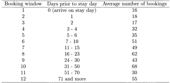
The challenge for a discrete time setting is how to appropriately pick the length for a time period. In other words, we need to decide what level of detail we should use to aggregate demand. First, due to the specialty in the booking patterns, a fixed length is likely to result in an imbalance among time windows in terms of booking quantities. On this account, we should use time windows with variant lengths so that the number of bookings in each window is about the same level. Moreover, too detailed levels should be avoided since they drag down the average demand, which would bring sizable variances into the booking patterns. Another thing to take into account is that the lengths of time windows should be appropriate for decision-makings as well. As the stay date gets close, we would prefer to adjust our decisions more frequently due to the importance of late bookings. Hence, the length should be shorter for time windows close to stay dates. Building on the discussions, we aggregate the booking horizon in our problem into 12 booking windows. The details are shown in Tab. 3.1 and a reference for the average number of bookings in each booking window is also provided.
The aggregation of demand raises another challenge on completing the missing information. In each booking windows, the aggregated booking quantity is given by the sum of bookings and the aggregated room rate is given by the average room rate. However, the data only provides us with the records related to existed bookings. For units that there exist no bookings, the corresponding room rates are lost, and we have to find ways to repair the data. One way to restore the price information is to use extrapolation, yet extrapolation is a limited method. It needs many data
Table 3.1: Details on the aggregation of booking windows and the average of number of bookings in each booking window
Booking window Days prior to stay day Average number of bookings
1 0 (arrive on stay day) 16
2 1 18 3 2 17 4 3-4 32 5 5-6 35 6 7- 10 51 7 11- 15 49 8 16-23 62 9 24-30 43 10 31-50 68 11 51-70 30 12 71 and more 55
points to estimate the missing values, and in our problem, this could only work for the major market segments where there is few booking windows missing pricing records. For other market segments where the total number of bookings is small, most of their booking windows are empty and only a few data points can be utilized for extrapolations. Hence, the extrapolation method is likely to fail in our case. To address this challenge, we adopt a simple method that replaces the missing column with zeros. In terms of prediction, filling in zeros brings output information into input variables, and it would undermine the convincingness of our prediction model. Nevertheless, the method is acceptable for our problem. In fact, most missing records are from the market segments with few bookings in general, so in terms of singling out these market segments, filling zeros is a reasonable method and will not impact our prediction results for other major market segments. In our numerical experiment, we also employ another method that removes all the rows with missing columns during aggregation. Some numerical results that compare these two methods are provided in the following sections.
The last challenge we need to address in preprocessing is the issue of lost sales. As explained in the previous chapter, the number of bookings we observe in the system is indeed adjusted through two steps. A portion of the demand might be rejected
due to historical capacity control decisions, creating discrepancies between the true demand and the historical booking records. Before using these bookings records, it is necessary to implement some reverse engineering methods to restore the lost sales. However, historical inventory controls are not provided in our data, and given that lost sales could happen even before the number of bookings hit the total capacity bound, restoring lost sales seems to be infeasible. We instead adopt a heuristics that removes from the data all the dates with occupancy greater than 98%, which is called a safe occupancy level. We will provide in the following sections the prediction results for the models that are trained on the truncated data for comparisons.
3.2
Prediction Model
Based on previous discussions, the demand to predict has been defined as the number of bookings in a given unit. The next step is to select features, or input variables, for our demand prediction model. After aggregation, each row of the data specifies a stay date, a booking unit (room class, market segment, booking window), a room rate (price) and the quantity of bookings. In addition, we include into the columns some extract features that corresponds to the stay dates: month (January, February, ... ) and day (Monday, Tuesday, ... ). These two factors are aimed to help estimate
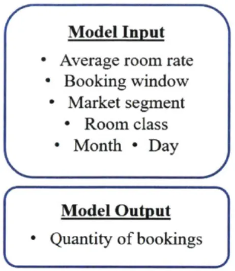
the unconstrained demand i.e. the number of bookings before adjusted by pricing constraints. Specifically, a list of features we select for our prediction model as well as the output variable are shown in Fig. 3-1.
It can be seen that our selection of features have covered all the basic information provided by the data, but it could be further improved from the following aspects. First of all, the only price factor in the model is the average room rate for a booking window. In reality, room rates from competing hotels can have significant impacts on the quantity of bookings, yet they are not included in the model due to the limit of the dataset. Secondly, as mentioned in the basic settings, the number of bookings in each unit is likely to be dependent on each other, so we could improve the model by incorporating room rates from units with similar features, which could be detected
Model Input - Average room rate
- Booking window - Market segment Room class - Month - Day Model Output Quantity of bookings
Figure 3-1: The input and output variables for our demand prediction model
through some clustering techniques. Lastly, the basic features might not be able to capture all the factors affecting the quantity of booking, and we are expected to incorporate more hand-made features by working collaboratively with the company.
We build a random forest regression model with all the given features. A random forest regression model
[7]
starts from developing regression trees, and the mechanism of trees can be understood as repeatedly selecting features to split the data until a further split can no longer add values to the prediction. To be specific, in the beginning of a tree model, it runs a value test for each feature (attribute) in which the data is partitioned into two subsets based on a threshold value of the attribute. Then the feature and its threshold value that have the best performance in terms of improving predictions are selected as the splitting criteria for the current level. In classification, predictions are produced by selecting the majority class, while in regression, prediction results are represented by the mean values of the output variable in a given subset. This process is repeated at each level, and it stops when the subset can no longer improve the prediction. In the end, a tree is built with each level providing a splitting criteria and each leaf (terminal node) providing a prediction result. Fig. 3-2 shows an example of a regression tree model.Random forest generalizes the idea of trees and it is an ensemble method. In a random forest, there are multiple subtrees and each subtree is built by using only a random portion of the data and a random subset of the attributes. The prediction
Booking window < 5?
I1
Average room rate < $ 250? Quantity I 1
Quantity Quantity
10 6
Figure 3-2: Illustrative example of a regression tree
result for a random forest is given by integrating the results of all the individual trees, such as using the mode (classification) or the mean prediction (regression). By sampling the training data, the attributes, and pooling the results, random forests are able to reduce an individual tree's over-fitting to the training set, as well as its prediction variance.
In the process of building a tree, it also helps reduce over-fitting by applying pruning methods, meaning to cut down the lower levels of the tree in order to reduce the model's dependency on training data sets. The degree of pruning is decided
by doing experiments on validation data sets. We can also obtain similar effect in
reducing over-fitting by stopping growing the tree at some point, for example, when the tree's height is too big, or when the number of nodes in a leaf is too small.
In our problem, we choose to build a random forest model for demand prediction because it has good interpretability. More importantly, as a tree-based model, it can deal with categorical variables and numerical variables at the same time. For models that can only have numerical variables as inputs, we either need to encode categorical variables into numeric values, or to develop models separately for each unique combination of the categorical variables. Both methods are consisted of a large number of parameters and will require a much bigger data set to train a good model. More discussions on the advantages and disadvantage of a random forest model are presented in the last section of this chapter.
3.3
Numerical Results
In the numerical experiments, we begin with splitting the data into two datasets: training and test. We are provided in the data with the booking history for a year, about 366 stay dates and their corresponding booking records for all units. After preprocessing, each date has 1020 rows and each row represents a unique combination of room class, market segment and booking window. Two thirds of the dates are randomly sampled for training and the remaining one third is for test, meaning there are 244 times 1020, in total 248,880 rows for training, and 124,4480 rows for test. Recall that in our model, the number of bookings for each stay date is assumed to be independent and takes its own booking records as inputs. Hence, we do not need to concern about the time sequence in sampling the data by stay dates. In our experiment, a portion of the training dataset will be used to run cross-validations in order to decide the hyper-parameters of the random forest model, like the number of subtrees, the minimum number of observations in a leaf node, etc.
Our random forest models are trained in R with a package called ranger, which provides a fast implementation as well as tools for variable importance analysis. More details on the package can be found in [28]. A tree-based model is criticized to be prone to overfitting when the tree grows too large. In training the model, we address this issue in two ways: first, for each subtree we limit the number of data points in a leaf node to be greater than a certain amount; second, we apply a bagging technique that samples both training data points and input variables to reduce the prediction variance caused by a single tree and its dominant features. Specifically in the experiment, we sample with replacement N data points (N is the total number of observations in the training data) to build a tree and randomly select 4 out of
6 input variables to split at each node. The minimum number of observations in a
terminal node is set as 25. We repeat this tree building process for 100 times in order to generate 100 trees, which construct a random forest, and all the parameters for our random forest model are selected by doing cross validation tests.
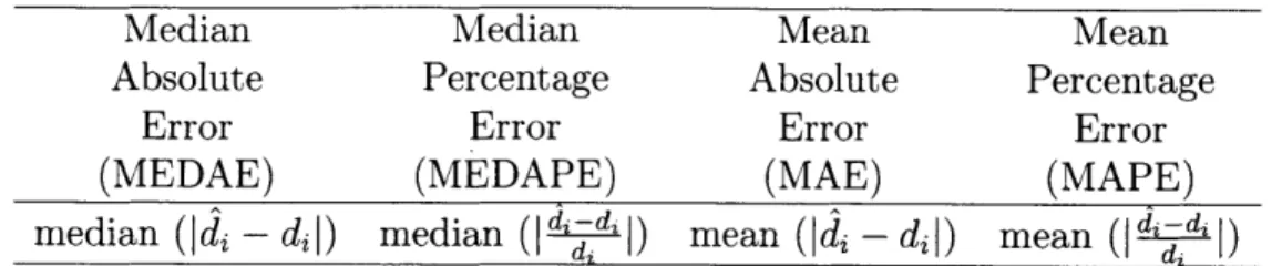
Table 3.2: Performance metrics
Median Median Mean Mean
Absolute Percentage Absolute Percentage
Error Error Error Error
(MEDAE) (MEDAPE) (MAE) (MAPE)
median (fdi - di| median (| i:-d|J) mean (ld - di|) mean (I di-di
a distribution on the quantity of bookings. The results can be converted into a probability distribution of demand, and we will see in Chapter 4 that these probability distribution estimations in fact can be used as inputs for a stochastic optimization model. Another way to use the results is to calculate the average of the predictions and use the expected values as the inputs for deterministic models. To show the prediction accuracy of our model, we take the average of the predictions as our estimation of demand and round them to integers.
A list of metrics we use to measure the performance is listed in Tab. 3.2. Let di denote the true quantity of booking, where i stands for a unique combination of
booking window, market segment and room class, and let di denote the prediction result of the random forest model. Then absolute error is expressed as
|di
- d l, and(absolute) percentage error is expressed as j - . The mean and median in the metric is taken across all the rows in the test data. Generally, percentage error shows an intuitive measure on the prediction accuracy. In our problem, however, the scale of demand is small, and even a small absolute error can result in a big percentage error. For example, when di = 1 and di = 4, the percentage error is 300%. It seems
to be an unacceptable error, but in practice, this would be considered as a good prediction. Therefore, we use both absolute error and percentage error to measure model performance, and consider median in addition to mean for median values are less sensitive to skewed data points than mean values.
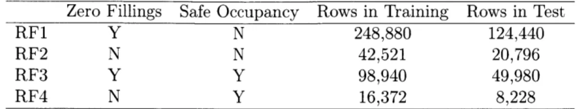
We compare four models in the experiments: RF1 and RF2 are trained on the data with all occupancy levels without removing the dates with occupancy greater than 98%, while RF3 and RF4 are trained on the data that only has dates with 'In the case where di = 0, we replace the percentage error with its corresponding absolute error to avoid involving infinite values.
Table 3.3: Dataset comparison for different models
Zero Fillings Safe Occupancy Rows in Training Rows in Test
RF1 Y N 248,880 124,440
RF2 N N 42,521 20,796
RF3 Y Y 98,940 49,980
RF4 N Y 16,372 8,228
Table 3.4: Prediction results comparison
MEDAE MEDAPE
(%)
MAE MAPE(%)
RF1 0 0 0.235 10.5
RF2 1 40.0 1.379 59.1
RF3 0 0 0.227 10.2
RF4 1 42.8 1.363 60.5
occupancy less or equal to 98%; RF1 and RF3 are trained on the data with zeros filling in the missing columns, while RF2 and RF4 are trained on the data with zero fillings removed. A comparison on the training and test dataset for different models is listed in Tab. 3.3. The prediction results on are shown in Tab. 3.4.
The results show that the random forest models trained with zero fillings (RF1,
RF3) have very good prediction performance. This is not surprising because these
models have taken advantage of the obvious pattern in the data that there is no booking under zero room rates. For models trained without zero fillings (RF2, RF4)
, the prediction accuracy decreases, but still in an acceptable range given that the
absolute errors are small. In fact, after preprocessing, there are only 16% of the rows that do not have zero room rates, which means the majority of bookings are from the minority of units with regular room classes and popular market segments. This observation suggests an aggregation of booking units for the purpose of reducing zero fillings and grouping market segments. As for the comparison on using safe occupancy levels, there is no significant difference in the prediction results. It can actually be observed that the hotel property we are given has high traffic: for over 60% of the days, the occupancy is over 98%, which suggests an adjustment on the safe occupancy level. Moreover, removing the dates with high occupancy levels might not be a good idea in this case, since it substantially reduces the available data points in the dataset.
0.45 18% 0.4 16% 0.35 14% 0.3 12% 0.25 10% 0.2 8% 0.15 6% 0.1 4% 0.05 2% 0 0% 1 2 3 4 5 6 7 8 9 10 11 12 1 2 3 4 5 6 7 8 9 10 11 12
Booking Window Booking Window
Figure 3-3: Distribution of prediction errors in all booking windows
Another observation we make is based on the distribution of prediction errors in different booking windows; see Fig. 3-3. The figure shows the mean absolute error and the mean percentage error in each booking window for model RF1. We can see that as the booking window gets smaller, i.e. the window gets closer to the stay date, predictions are more accurate. The results can be explained in two ways: first, for the late booking periods, as the number of bookings increases, customers' booking patterns are more evident and thus can be captured by our forecast model, while in the beginning periods, the pattern is obscure; second, the aggregation of booking windows is more detailed for late booking periods, while for early booking windows, the demand-price relationship is subject to distortions due to asymmetrical aggregations. The observation suggests a room for improvement for our method of aggregating demand. In Appendix A, we report more results on the prediction errors of different models.
To justify our selection of features, we also run some experiments to analyze the importance of variables in our prediction models. In general, there are two ways to estimate variable importance in a regression tree (and a random forest as well): Gini importance and permutation importance. Gini importance for a random forest measures the average decrease in node impurities over all tree in the forest, and for regression models, node impurity is calculated based on the variance of responses. Permutation importance uses a permutation technique conditioning on correlated features, and it measures the difference in prediction accuracy before and after the
*'"Booking Window Room Class 17%
r6%
Room Rate Room Rate 10% 40%UD
2%Booking Window m Room Rate w Month m Booking Window n Room Rate s Month * Day a Market Segment N Room Class * Day 0 Market Segment m Room Class
Model RF1 Model RF2
Figure 3-4: Variable importance analysis for our prediction models
permutation test. Further details explaining these methods can be found in [23] [24]. In the following, we will provide the results of permutation importance for model
RF1 and RF2. In Fig. A-2, we plot out the relative importance of different variables
in percentage. It can be seen that for model RF1, since the training data include the obvious pattern associated with filling zeros, room rate is the most important variable for predictions. For model RF2, as we remove the rows with missing prices, the relative importance of room rate decreases, while room class and market segment become the most important variables. These variables being important also suggests that the demand-price relationships in different booking units could be very different. Furthermore, in both models, day and month factors seem to be less impactive, which suggests the exploration of other day features. The results for Gini importance are reported in Appendix A.
3.4 Discussion
We close the chapter with some discussions on the advantages and disadvantages of using random forest models, or more broadly tree-based models, for demand predic-tions in general operation management problems.
First and foremost, the obvious benefit of using random forest models is that they do not require any specific parametric functional forms, which means they can work for more general demand patterns. This nonparametric structure has been called as algorithmic modeling in
18]
that discusses the two cultures in statistical modeling. Compared to traditional data modeling methods which assumes functional forms, algorithmic modeling methods relax the functional constraints and are thus more flexible. In the context of predicting demand price relationship, for example, common techniques would require demand to be a decreasing function of price, whereas for random forest regression models, such requirements are not necessary. In fact, in some operation management problems where prices serve as a signal of quality, demand might even increase with price; see1151.
In these cases, tree-based models or other nonparametric models can capture the patterns between demand and price effectively. The flexibility of random forest models is also reflected in their ability in deal-ing with numerical and categorical variables at the same time. For problems with underlying patterns that vary with categories, random forest saves the complexity of building models separately for each category, and they do not require encoding categorical variables into numerical ones. Take our problem as an example, the rela-tionship between demand and price in different booking units can be very distinct as suggested by Fig. A-2. In a random forest model, these variations can be easily and well captured by the paths from a tree's root node to its terminal nodes. In addition, random forests are equipped with variable importance metrics, which could provide critical insights in selecting features and distinguishing important features from the less impactive ones.Another benefit we can obtain from random forest models is that they have good predictability as an ensemble method. As explained previously, a random forest implements bagging methods both in developing subtrees and in selecting features to split. This bagging technique helps avoid the over-fitting nature of a single tree and reduces the variance in prediction results, contributing to a random forest's good predictability. There also exit some other ensemble methods that might be helpful in developing a regression model, like boosting, Bayesian averaging, and see
1121
for abrief review and the details about these methods.
Last but not least, random forest models are easy to interpret. The structure of trees is simple and intuitive, where prediction results are produced by checking the splitting rules at each node; see Fig. 3-2. In a business environment, random forest are more favorable than other machine learning techniques like neural networks because
it avoids offering a black box. A tree-based model's good interpretability can also
help provide managerial insights.
In terms of disadvantages, firstly, the non-parametric structure of random forest models results in a more challenging optimization problem, as we will see in the fol-lowing chapter. Random forest models generate predictions in a one-to-one mapping manner rather than using parametric functions. Therefore, in our problem, the pric-ing decisions that appear as an input feature of the random forest have to be modeled as discrete variables in the optimization formulations, and these formulations tend to be more difficult to solve.
Another factor that might prevent the use of random forest models is the lack of data of high quality. As we have shown in the previous modeling steps, it requires a rich dataset to train a random forest and run cross validation tests to decide the hyper-parameters in the model. In many practical problems, the data is not managed in a scientific way and only a small amount of qualified data can be used for building a machine learning model. (like in our problem, pricing records for days without bookings are lost.) In these cases, the performance of a nonparametric model will be very limited.
The last criticism for random forest and other tree-based models is that they are very likely to be over-fitting to the training dataset. Though techniques like bagging and pruning can help reduce the effect, they could not solve the problem essentially. The intrinsic nature of trees and random forests indeed results from its greedy selection of features while determining the splitting rules. At each node, a tree always picks the feature to split that gives the best immediate improvement, while ignoring the gains in future splits. This greedy manner makes the model prone to over-fittings. In fact, there are some innovative methods on resolving this local
optimality issue and developing robust, globally optimal trees. See [5j
[6]
for the related works.In the next chapter, we will explain our optimization models for selecting pricing and capacity allocation decisions that maximize revenue. We will adopt the prediction model we have developed in this chapter to forecast the number of bookings under given prices, and then plug the prediction results into optimization models to find the optimal solutions. More details on the formulations as well as the algorithms are explained in the following.
Chapter 4
Decision Optimization
In this chapter, we will discuss the optimization models for the pricing and capacity allocation decisions of a hotel property. To begin with, we will introduce a simple finite-stage Markov decision framework as the underlying structure and discuss the dynamic programming algorithm. Due to the curse of dimensionality, solving dynamic programming models becomes challenging as we increase the scale of the problem. So in the next step, we will build a deterministic integer programming model instead to simplify the formulation. We also show that the integer program can be solved as an linear program equivalently. In the numerical experiment, we will adopt the prediction model developed in Chapter 3 to forecast demand under given prices, and then plug the predictions into our optimization model to find the optimal solutions. Numerical results are provided to show the significant increase in revenue with opti-mized decisions. In the last, we will discuss the possibilities of solving our problem using the approximate dynamic programming approach. We will close the chapter with some discussions on how to implement different algorithms in practice.
4.1
Markov Decision Framework
A Markov decision process (MDP) is a discrete time stochastic control process, where
at each time step, decision makers choose an action given the current state, and then randomly move into a new state with a corresponding reward. The probability of such
a state transition only depends on the current state and the decision maker's action, and is conditionally independent of all previous states and actions, which satisfies the Markov property. A Markov decision process is consisted of the following five components: a finite set of states S, a finite set of actions (controls) A, transition
probabilities Pa(s, s') = Pr(st+i = s'Ist = s, at = a) representing the probability of
moving into state s' at time t + 1 from state s at time t under action a, immediate rewards Ra(S, s') resulted from the transition from s to s' due to action a, discount
factor -y E [0, 1] which represents the difference between future rewards and present rewards. The goal in an MDP problem is to find a policy function T(s), a mapping from states to optimal controls that maximize the expected cumulative rewards over a potentially infinite horizon:
E{ E y'Ra, (St st+1)}. (4.1)
t=O
To translate the pricing and capacity control problem into an MDP model, we need to appropriately define its components. We begin with a simple case where there is only one room class and one market segment. First notice that we only have finite many stages in our problem, so the discount factor can be set as 1, without raising any convergence issue. To make it consistent with the booking windows defined in previous chapters, we reverse the time index here and assume that the decision window starts from period T and ends with period 0.
We define state Xt as the remaining capacity for the given room class at time period
t, pt as the actions denoting the price (room rate) being charged at time t, and yt the
number of rooms allocated to time t for the given market segment. To have a finite number of states and controls, xt and yt are assumed to be discrete variables. Also,
xt is from set X = {0, 1, ..., S} and pt is from set P = {P1,P2, ---,PN}- S is defined as
the total room capacity and N is the number of admissible prices. In addition, yt is
further assumed to belong to the set (0, ... , xt}, which means overbooking is excluded from our considerations.