Neural Networks for Cross-Section Segmentation in Raw Images of Log Ends

HAL Id: hal-03058259

https://hal.archives-ouvertes.fr/hal-03058259

Submitted on 11 Dec 2020

HAL is a multi-disciplinary open access

archive for the deposit and dissemination of

sci-entific research documents, whether they are

pub-lished or not. The documents may come from

teaching and research institutions in France or

abroad, or from public or private research centers.

L’archive ouverte pluridisciplinaire HAL, est

destinée au dépôt et à la diffusion de documents

scientifiques de niveau recherche, publiés ou non,

émanant des établissements d’enseignement et de

recherche français ou étrangers, des laboratoires

publics ou privés.

Neural Networks for Cross-Section Segmentation in Raw

Images of Log Ends

Rémi Decelle, Ehsaneddin Jalilian

To cite this version:

Rémi Decelle, Ehsaneddin Jalilian. Neural Networks for Cross-Section Segmentation in Raw Images

of Log Ends. Fourth IEEE International Conference on Image Processing, Applications and Systems

(IPAS 2020), Sep 2019, Gênes, Italy. �hal-03058259�

Neural Networks for Cross-Section Segmentation in

Raw Images of Log Ends

R´emi Decelle

Universit´e de Lorraine, LORIA, UMR 7503, 54506 Vandoeuvre-l`es-Nancy, France remi.decelle@loria.fr

Ehsaneddin Jalilian

Abstract—In this paper, wood cross-section (CS) segmentation of RGB images is treated. CS segmentation has already been studied for computed tomography images, but few study focuses on RGB images. CS segmentation in rough log ends is an important feature for the both assessment of wood quality and wood traceability. Indeed, it allows to extract other features like pith, eccentricity (distance between the pith and the geometric centre) or annual tree rings which are related to mechanical strength. In image processing, neural networks have been widely used to solve the problem of objects segmentation. In this paper, we propose to compare different state-of-the-art neural networks for CS segmentation task. In particular, we consider U-Net, Mask R-CNN, RefineNet and SegNet. We create an imageset which has been split into 6 subsets . Considered neural networks have been trained on each subset in order to compare their performance on different type of images. Results show different behaviors between neural networks. On the one hand, overall U-Net learns better on small dataset than the others. On the other hand, RefineNet learns well on huge dataset. While SegNet is less efficient and Mask R-CNN does not provide a detailed segmentation. This offers a preliminary result on neural network performances for CS segmentation.

Index Terms—Deep convolutional neural networks, Pixel-wise segmentation, Wood quality, Sawmill scenes

I. INTRODUCTION

In this paper, we focus on neural networks to segment wood section (CS). There are few publications on wood cross-section analysis with RGB camera. Cross-cross-section analysis focuses on computed tomographic (CT) images which allow to estimate both external and internal characteristics. Those characteristics can be used to estimate wood quality. More precisely, the wood quality is defined by some properties [1] among which:

• mechanical resistance;

• dimensional stability. Wood is hygroscopic meaning that it can gain or lose moisture from the surrounding air that could be source of trouble;

• durability, that is the ability to resist to fungi and insects without chemical treatments;

• aesthetic for furniture or apparent beams in building (looking forward to regularity in tree rings).

All of these characteristics are unfortunately not directly measurable on CS images. However, they can be estimated by obtaining intermediate characteristics which are visible on

images. For instance, annual tree ring width is an indication to wood mechanical properties [2].

A lot of techniques have been proposed to segment CS on timber trucks or log stacked in a pile [3]–[5]. Samdangdech et al. [4] used neural network to segment log-end on timber trucks. For such task, a dataset with log pile images have been proposed [6]. But, our task is different as there is one CS (or very few CS) in our images (see Figure1). Our images are taken close to the CS contrary to log pile or timber trucks.

(a) Log file from [6] (b) Ground truth for 1a

(c) Image from our imagesets (d) Ground truth for 1c

Fig. 1: Examples of images from a log pile and our imageset. To estimate the wood features we need to segment, in the images, the cross-section from the background. In addition to a high segmentation accuracy, the time performance is also a high criteria for real world applications (industry or scientific applications). To our knowledge, for segmenting automatically the CS only one method have been assessed [7].

The proposed method in [7] to segment cross-section of spruce1_{, is based on similarity of image sections and requires}

pith estimation. Image is divided into small blocks. Then, we analyse each block in terms of texture features. All blocks sharing the same texture features as those close to the pith

belong to the cross-section. It provides accurate results and requires around one second to estimate the cross-section segmentation. But there are two drawbacks to this method. On the one hand, it suffers of time computation. The method is coarsely linear in scale but reducing block size by 2 may increase up to 4 the time computation. On the other hand, it also requires the pith position (which is done automatically in their method). This latter task may be difficult on images of rough CS. Furthermore, texture analysis is processed in grayscale (color information is lost).

In the field of computer vision, a lot of methods have been proposed to segment images. But recently, neural networks seem to outperform all those methods. We propose in this paper to evaluate few convolution neural networks for this task. Indeed, neural networks can compute fastly the segmentation of the cross-section which is an important criteria in sawmill environment. Moreover they have shown their performances in others similar tasks.

The paper is organized as follows. First, Section II describes each proposed neural networks. Then, Section III details im-agesets and Section IV shows results. We conclude in Section V.

II. ARCHITECTURE OF THE PROPOSED CONVOLUTIONAL NEURAL NETWORKS

There are a lot of convolutional neural network (CNN) for image segmentation. In this paper, we propose to evaluate few CNNs which have provided good results for segmentation task. The proposed CNNs are: a modified version of U-Net [8], Mask R-CNN [9], RefineNet [10] and SegNet [11].

A. U-Net Architecture

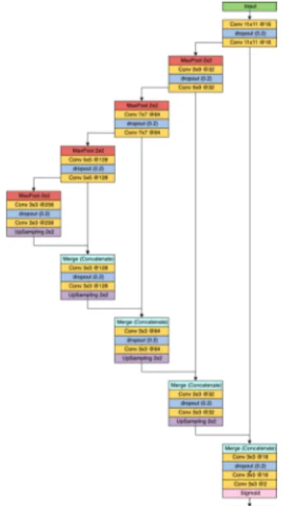
The first CNN we trained was adapted from the U-Net network proposed by Ronneberger et al. [8]. It has been chosen since it is known to learn fast and to provide good results. Moreover, it requires less data for the training. It is composed of a contracting path and an expanding path. The network architecture is illustrated on Figure 2. The main changes we did are on the contracting path: dropout layers were introduced and convolution filter size are larger than the original version. These following changes are based on experimental results.

The contracting path consists of one 11 × 11 convolution (original was3 × 3), a dropout, a second 11 × 11 convolution and a 2 × 2 max pooling with stride 2 for downsampling. Each convolution is followed by a rectified linear unit (ReLU) function and each dropout probability is set to0.2. For the first block, there are 16 convolution filters. At each downsampling, we twofold the number of convolutions filters and reduce their size by 2, down to a size of3 × 3 (i.e. 11 × 11, then 9 × 9, 7 × 7, 5 × 5 and 3 × 3).

The expanding path consists of an upsampling of feature map followed by2×2 convolution which halves the number of filters, a concatenation with the cropped feature map from the contracting path and finally one3 × 3 convolution, a dropout and an other_{3 × 3 convolution (each convolution is followed} by a ReLU). At the end, a 3 × 3 convolution with 2 filters

is done first and a 1 × 1 convolution with 1 filter is secondly done, which is equivalent to a sigmoid function.

We set ADAM optimizer for the training with a learning rate set at 0.0001 and the loss is the binary cross entropy.

Fig. 2: Architecture of the applied CNN based on U-Net.

B. Mask R-CNN Architecture

The second CNN is Mask R-CNN [9]. This network is more complex than the previous one (see Fig.3). It aims at detecting and classifying different objects in images. It is an extension to Faster RCNN [12]. Contrary to Faster RCNN which only classes and creates a bounding-box, Mask R-CNN provides a segmentation for each detected object. Mask R-CNN has two main stages. First, the network has to create regions where there might be an object to detect. This stage is called Region Proposal Network. Second, it predicts the class of each detected regions (using a RoIPool) and generates a binary mask for these regions. Both stages are connected to a backbone structure. The backbone is also an neural network.

The used backbone is ResNet-101-FPN. It was pre-trained with MS COCO datasets. No modifications were provided on this CNN [13].

C. RefineNet Architecture

The third CNN used is RefineNet [10]. The network is a multi-resolution refinement network, which employs a 4-cascaded architecture with 4 Refining units, each of which directly connects to the output of one Residual net [14] block, as well as to the preceding RefineNet block in the cascade (see Fig.4). Each Refining unit consists of two residual convolution units (RCU), which include two alternative ReLU and _{3 × 3 convolutional layers. The output of the RCU} units are processed by 3 × 3 convolution and up-sampling

Fig. 3: Architecture of Mask R-CNN (source from [9]).

layers incorporated in multi-resolution fusion blocks. A chain of multiple pooling blocks, each consisting a 5 × 5 max-pooling layer and a 3 × 3 convolution layer, next operate on the feature maps, so that one pooling block takes the output of the previous pooling block as input. Therefore, the current pooling block is able to re-use the result from the previous pooling operation and thus access the features from a large region without using a large pooling window. Finally, the outputs of all pooling blocks are fused together with the input feature maps through summation of residual connections. We used ADAM optimizer with learning rate of 0.0001, in 40, 000 epoch iteration to train the network. The implementation of this network was realized in the Keras library using TensorFlow back-end [15].

Fig. 4: Big picture of the architecture of RefineNet (source from [10]).

D. SegNet Architecture

The last CNN in this paper is identical to the basic fully convolutional encoder-decoder network proposed by Kendall et al. [11] and is termed ”SegNet” subsequently (see Fig.5). However, we redesigned the softmax layer to segment only the vein pattern. The whole network architecture is formed by an encoder network, and the corresponding decoder network. The network’s encoder architecture is organized in four stocks, containing a set of blocks. Each block comprises a convolu-tional layer, a batch normalization layer, a ReLU layer, and a pooling layer with kernel size of 2 × 2 and stride 2. The corresponding decoder architecture, likewise, is organized in four stocks of blocks, whose layers are similar to those of the

encoder blocks, except that here each block includes an up-sampling layer. In order to provide a wide context for smooth labeling in this network the convolutional kernel size is set to 7 × 7. The decoder network ends up to a softmax layer which generates the final segmentation map.

We used Stochastic Gradient Distance (SGD) optimizer with learning rate of 0.003, in 30,000 epoch iteration to train the network. The implementation of this network was realized in caffe library [16].

Fig. 5: Architecture of SegNet (source from [11]).

E. Other Methods

We implemented two other methods for image segmenta-tion. The first one is K-means [17], and the second one is active contour [18] (also called snake). For both of them, we first resized images to a size of 512 × 512, then we applied a gaussian filter with σ = 2.5 and processed in the CIELAB color space. For the K-means method, we set K = 5. The cross-section is the largest circular object. The circularity is computed by the formulae:

Circularity = (4 ∗ A ∗ π)/(Perimeter2₎

And for the active contour method, we setµ = 0.5 and ν = 0. The initial snake is a circle centered in the image with a radius of 128.

III. EXPERIMENTALMETHOD

A. Imagesets

To the best of our knowledge, there is no dataset available for our task. We created our own imageset. The full imageset consists of 2381 images of wood log end cross-sections. The imageset is composed of two species: Norway spruce and Douglas fir.

It consists of 6 different subsets: 3 subsets composed of spruce and 3 composed of Douglas fir. Each subset is composed with images captured by a same camera. We split the imageset because images have been captured by 6 different cameras at different stages during log process (after harvesting, on the log yard, before sawing). More precisely, there are three main differences between each subset:

• ambient light between outdoor and in sawmill condi-tions;

• color between fresh sew wood and wood left on log yard for few weeks;

• color differences between both species (uniform color of spruce, red heart of Douglas fir).

Fig.6 shows few samples for each subset. Moreover, the total number of images per camera are highly different. For instance, one camera has captured more than 1,000 images and another one has only captured 11 images. Table I details each subset camera device model, total number of captured images, size of images and specie. Including all those images in a single dataset would have led to an unbalanced dataset.

Fig. 6: Some images from the six subsets. The first row Ane subset (Douglas fir),2nd

row Huawei subset (Spruce),3rd

row Lumix subset (Douglas fir),4th

row Sawmill subset (Douglas fir),5th

row sbgTS3 subset (Spruce) and the last row sbgTS12 subset (Spruce).

B. Data Augmentation

As each subset has its own properties (color, contrast and so on) and some subsets are really small, we always proceeded to a data augmentation for the training. This allows a more robust training for the networks. Random deformations are proceeded: scaling, rotation, vertical and horizontal shift,

TABLE I: Total number of images and image size for each camera.

Subset Name sbgTS3 sbgTS12 Camera Canon EOS 70D Canon EOS 5D Mark II Number of images 1504 768

Image’s size 1368 × 912 2048 × 1365 Wood specie Spruce Spruce Subset Name Sawmill Lumix

Camera Sawmill camera Panasonic DMC-FZ45 Number of images 39 37

Image’s size 5472 × 3648 4320 × 3240 Wood specie Douglas fir Douglas fir Subset Name Huawei Ane

Camera Huawei PRA-LX1 Huawei ANE-LX1 Number of images 22 11

Image’s size 3968 × 976 4608 × 3456 Wood specie Spruce Douglas fir

zooming and shearing. Each model has been trained on the 6 subsets. We applied a 2-fold cross-validation on each subset.

C. Evaluation Method

Ground truths have been manually assessed by different operators. Ground truth is the CS without the bark. To compare the neural networks we use 8 metrics. Let TP be true positives, TN be true negatives, FP be false positives and FN be false negatives, we compute these metrics according to the followings equations: P recision = T P T P + F P Recall = T P T P + F N Dice = 2 ∗ T P 2 ∗ T P + F P + F N Accuracy = T P + T N T P + T N + F P + F N IoU = T P T P + F P + F N N ice2 = 1 2( F N F N + T P + F P F P + T N) M CC = T P × T N − F P × F N√ P where P = (T P + F P )(T P + F N )(T N + F P )(T N + F N ) As, for some subsets, classes are unbalance, accuracy is not enough to compare networks. Indeed, in images from Sawmill subset the cross-section is small compared to background (see Figure 6). This is the reason why we compute precision, recall, dice, accuracy, Intersection over Union (IoU), Nice2 and Matthews Correlation Coefficient (MCC) in order analyse neural network results.

MCC is the least biased score to evaluate networks. It is interpreted as the correlation between the predictions and the ground truths [19]. Contrary to MCC, Nice2 indicates whether

there are a lot of wrong estimation and IoU allows to observe if the segmentation overlaps the ground truths. Accuracy and Dice also indicate whether the segmentation is accurate but only in case where foreground and background are balanced.

IV. RESULTS

A. Global overview

Table II shows performance for the different neural networks and for each subset. The differences between models are highlighted by those results.

First, MCC indicates that RefineNet performs well for Ane,

Sawmill, sbgTS12 and sbgTS13 subsets, U-Net performs better on Lumix subset and Mask R-CNN is the more suitable on

Huaweisubset. It can be observed that SegNet is outperformed by others networks for each subset. However, its MCC is close to the others. The non-deep learning methods performs well on Ane, Huawei and Lumix. However, they are worst for the

Sawmill imageset. Indeed, the cross-section is small in those images and images are low in constrast, which leads these methods to overestimate the cross section. This is indicated by their high value of recall and accuracy.

Another interesting observation is that Mask R-CNN often has the highest precision but it has a lower value for the other scores. It indicates that its pixel prediction is very accurate but it struggles to detect all the pixels belonging to the CS.

Contrary to Mask R-CNN, U-net has a higher recall than precision. It seems that U-Net detects better CS in space but it underestimates the CS segmentation itself. This is confirmed by the low Nice2 and low IoU. However, U-Net has very low scores on Sawmill subset. For this subset, CS are very small leading to an unbalance in classes. U-Net struggles to detect and to segment cross-section on such images. It performs better when CS are bigger in images as in Lumix subset.

RefineNet gives in general best results. It outperforms others for both sbgTS3 and sbgTS12 subsets. Nonetheless, when the dataset is smaller RefineNet struggles to provide an accurate segmentation.

SegNet is never the best networks, but it is also never the worst. For Sawmill subset, SegNet is able to segment cross-section. But for Lumix subset is not the case.

Table III shows time computation for all methods. For the benchmarking, we use 16GB RAM with 2133 MHz (LPDDR3), a processos Intel Core i7 and Intel Iris Plus Graphics 640 1536 Mo as graphic card. Neither GPU were used for deep-learning method nor for non deep-learning methods. K-means is the fastest method and the snake is the slowest method.

B. Detailled Analysis

To understand precisely each models strengths and weak-nesses, a detailed analysis was conducted. An important aspect in CS segmentation is to retrieve the shape.

Fig.7 shows model predictions in a non-trivial image. The log end is clearly not circular. U-Net underestimates log-end but retrieves precisely the shape of the cross-section. Mask R-CNN is less precise. It overestimates the shape in some areas

TABLE II: Performance overview for the models for each subset.

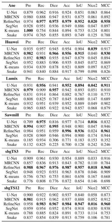
Ane Pre Rec Dice Acc IoU Nice2 MCC U-Net 0.879 0.962 0.916 0.924 0.851 0.063 0.864 MRCNN 0.980 0.888 0.947 0.931 0.875 0.061 0.892 RefineNet 0.974 0.977 0.975 0.979 0.952 0.020 0.958 SegNet 0.928 0.951 0.936 0.949 0.886 0.047 0.897 K-means 1.000 0.754 0.844 0.894 0.753 0.124 0.801 Snake 0.974 0.765 0.855 0.893 0.749 0.125 0.788 Huawei Pre Rec Dice Acc IoU Nice2 MCC U-Net 0.935 0.957 0.945 0.954 0.904 0.039 0.917 MRCNN 0.982 0.931 0.966 0.956 0.915 0.040 0.930 RefineNet 0.892 0.983 0.935 0.947 0.879 0.045 0.894 SegNet 0.952 0.883 0.906 0.935 0.845 0.072 0.869 K-means 0.934 0.839 0.878 0.921 0.809 0.097 0.827 Snake 0.941 0.840 0.884 0.917 0.799 0.098 0.826 Lumix Pre Rec Dice Acc IoU Nice2 MCC U-Net 0.931 0.956 0.941 0.952 0.894 0.042 0.911 MRCNN 0.979 0.909 0.957 0.942 0.893 0.051 0.910 RefineNet 0.831 0.914 0.864 0.882 0.767 0.110 0.773 SegNet 0.808 0.825 0.787 0.845 0.680 0.147 0.689 K-means 0.932 0.951 0.939 0.952 0.889 0.049 0.902 Snake 0.965 0.885 0.922 0.942 0.857 0.068 0.879 Sawmill Pre Rec Dice Acc IoU Nice2 MCC U-Net 0.709 0.975 0.816 0.977 0.714 0.016 0.832 MRCNN 0.994 0.907 0.995 0.948 0.901 0.047 0.946 RefineNet 0.984 0.951 0.959 0.996 0.936 0.024 0.961 SegNet 0.928 0.969 0.946 0.994 0.900 0.174 0.944 K-means 0.185 0.934 0.306 0.771 0.183 0.153 0.352 Snake 0.132 0.825 0.225 0.700 0.128 0.242 0.246 sbgTS3 Pre Rec Dice Acc IoU Nice2 MCC U-Net 0.909 0.961 0.930 0.954 0.889 0.033 0.916 MRCNN 0.857 0.836 0.913 0.843 0.782 0.110 0.784 RefineNet 0.988 0.967 0.976 0.987 0.957 0.018 0.968 SegNet 0.948 0.923 0.931 0.963 0.878 0.046 0.909 K-means 0.756 0.783 0.753 0.861 0.658 0.167 0.668 Snake 0.776 0.808 0.776 0.872 0.654 0.146 0.698 sbgTS12 Pre Rec Dice Acc IoU Nice2 MCC U-Net 0.900 0.922 0.902 0.937 0.840 0.058 0.873 MRCNN 0.981 0.915 0.962 0.937 0.888 0.052 0.912 RefineNet 0.958 0.983 0.967 0.984 0.947 0.016 0.960 SegNet 0.959 0.954 0.952 0.974 0.918 0.030 0.938 K-means 0.788 0.885 0.824 0.891 0.733 0.114 0.753 Snake 0.837 0.854 0.839 0.913 0.759 0.106 0.781

TABLE III: Time computation in ms for the models.

U-Net MRCNN RefineNet SegNet K-means Snake 466 1245 1143 911 341 2052

(bottom) and underestimates in other areas (top). RefineNet retrieves the CS shape but suffers from defects at image borders. Such defects are not highlighted in results shown in Table II. And SegNet estimates the cross-section with few gaps in the segmentation (bottom left). It can be observed that both U-Net and Mask R-CNN provide a smooth segmentation, which is not the case for RefineNet and SegNet. Both K-means and the snake method underestimate the cross-section and have holes within their segmentation.

Another image from sbgTS3 subset is used to underline networks differences. In Fig.8, the cross-section is next to other ones which must not be segmented. Like the previous images, both U-Net and Mask R-CNN provide a smooth segmentation. Contrary to the previous images, U-Net some-times overestimates the cross-section, but globally segments well. Mask R-CNN struggles with the snow (top left) as well as RefineNet. But Mask R-CNN includes the snow unlike RefineNet. The segmentation provided by SegNet far from the ground truth (too many FP). K-means let holes within its segmentation and underestimates the cross-section. Due to the snow, the snake method includes part of the adjacent cross-sections.

V. CONCLUSION

Despite the small size of some datasets, U-Net, Mask R-CNN, RefineNet and SegNet produce quite good segmentation of cross-section. RefineNet is better in general but it sometimes makes errors which could lead to huge errors. Contrary to RefineNet, U-Net provides a smooth segmentation and man-ages to provide fine segmentation with small datasets. But it is less accurate in general. Mask R-CNN struggles with complex shape and SegNet suffers from defects (like gaps in the shape). K-means should be considered is the time computation is the key point as K-means can provide a coarse cross-section. However active contour seems to be less accurate and is slower than others methods. Future works should focus on increasing the number of dataset to understand precisely each network strengths and weaknesses.

ACKNOWLEDGMENT

This research was made possible by support from both the French National Research Agency and the Austrian Science Fund (FWF), in the framework of the project TreeTrace, ANR-17-CE10-0016 and FWF International Project I-3653.

REFERENCES

[1] J. Barnett and G. Jeronimidis, Wood quality and its biological basis. John Wiley & Sons, 2009.

[2] K. J. Niklas and H.-C. Spatz, “Worldwide correlations of mechanical properties and green wood density,” American Journal of Botany, vol. 97, no. 10, pp. 1587–1594, 2010.

[3] B. Galsgaard, D. H. Lundtoft, I. Nikolov, K. Nasrollahi, and T. B. Moeslund, “Circular hough transform and local circularity measure for weight estimation of a graph-cut based wood stack measurement,” in

2015 IEEE Winter Conference on Applications of Computer Vision. IEEE, 2015, pp. 686–693.

[4] N. Samdangdech and S. Phiphobmongkol, “Log-end cut-area detection in images taken from rear end of eucalyptus timber trucks,” in 2018

15th International Joint Conference on Computer Science and Software Engineering (JCSSE). IEEE, 2018, pp. 1–6.

(a) Input (b) Ground truth

(c) UNet output (d) MRCNN output

(e) RefineNet output (f) SegNet output

(g) K-means output (h) Snake output

Fig. 7: Model predictions on an image from Huawei subset. Green pixels are TP, blue pixels are FN and red pixels are FP.

[5] Y. V. Chiryshev, A. V. Kruglov, and A. S. Atamanova, “Automatic detection of round timber in digital images using random decision forests algorithm,” in Proceedings of the 2018 International Conference on

Control and Computer Vision, 2018, pp. 39–44.

[6] C. Herbon, “The hawkwood database,” arXiv preprint arXiv:1410.4393, 2014.

[7] R. Schraml and A. Uhl, “Similarity based cross-section segmentation in rough log end images,” in IFIP International Conference on Artificial

Intelligence Applications and Innovations. Springer, 2014, pp. 614–623. [8] O. Ronneberger, P. Fischer, and T. Brox, “U-net: Convolutional networks for biomedical image segmentation,” in International Conference on

Medical image computing and computer-assisted intervention. Springer, 2015, pp. 234–241.

[9] K. He, G. Gkioxari, P. Doll´ar, and R. Girshick, “Mask r-cnn,” in

Proceedings of the IEEE international conference on computer vision, 2017, pp. 2961–2969.

[10] G. Lin, A. Milan, C. Shen, and I. Reid, “Refinenet: Multi-path refinement networks for high-resolution semantic segmentation,” in Proceedings of

the IEEE conference on computer vision and pattern recognition, 2017, pp. 1925–1934.

(a) Input (b) Ground truth

(c) UNet output (d) MRCNN output

(e) RefineNet output (f) SegNet output

(g) K-means output (h) Snake output

Fig. 8: Models predictions on an image from sbgTS3 subset. Green pixels are TP, blue pixels are FN and red pixels are FP.

[11] V. Badrinarayanan, A. Kendall, and R. Cipolla, “Segnet: A deep con-volutional encoder-decoder architecture for image segmentation,” IEEE

transactions on pattern analysis and machine intelligence, vol. 39, no. 12, pp. 2481–2495, 2017.

[12] S. Ren, K. He, R. Girshick, and J. Sun, “Faster r-cnn: Towards real-time object detection with region proposal networks,” in Advances in neural

information processing systems, 2015, pp. 91–99.

[13] W. Abdulla, “Mask r-cnn for object detection and instance segmentation on keras and tensorflow,” https://github.com/matterport/Mask RCNN, 2017.

[14] K. He, X. Zhang, S. Ren, and J. Sun, “Deep residual learning for image recognition,” in Proceedings of the IEEE conference on computer vision

and pattern recognition, 2016, pp. 770–778. [15] F. Chollet et al., “Keras,” https://keras.io, 2015.

[16] Y. Jia, E. Shelhamer, J. Donahue, S. Karayev, J. Long, R. Girshick, S. Guadarrama, and T. Darrell, “Caffe: Convolutional architecture for fast feature embedding,” arXiv preprint arXiv:1408.5093, 2014. [17] D. Arthur and S. Vassilvitskii, “K-means++: the advantages of careful

seeding, p 1027–1035,” in SODA’07: proceedings of the eighteenth

annual ACM-SIAM symposium on discrete algorithms. Society for In-dustrial and Applied Mathematics, Philadelphia, PA, 2007.

[18] T. F. Chan and L. A. Vese, “Active contours without edges,” IEEE

Transactions on image processing, vol. 10, no. 2, pp. 266–277, 2001. [19] D. M. Powers, “Evaluation: from precision, recall and f-measure to roc,