Multiple steady-states in the terrestrial atmosphere-biosphere system: a result of a discrete vegetation classification?

(1)

HAL Id: hal-00297876

https://hal.archives-ouvertes.fr/hal-00297876

Submitted on 22 Feb 2007

HAL is a multi-disciplinary open access

archive for the deposit and dissemination of sci-entific research documents, whether they are pub-lished or not. The documents may come from teaching and research institutions in France or abroad, or from public or private research centers.

L’archive ouverte pluridisciplinaire HAL, est destinée au dépôt et à la diffusion de documents scientifiques de niveau recherche, publiés ou non, émanant des établissements d’enseignement et de recherche français ou étrangers, des laboratoires publics ou privés.

Multiple steady-states in the terrestrial

atmosphere-biosphere system: a result of a discrete

vegetation classification?

A. Kleidon, K. Fraedrich, C. Low

To cite this version:

A. Kleidon, K. Fraedrich, C. Low. Multiple steady-states in the terrestrial atmosphere-biosphere sys-tem: a result of a discrete vegetation classification?. Biogeosciences Discussions, European Geosciences Union, 2007, 4 (1), pp.687-705. �hal-00297876�

(2)

BGD

4, 687–705, 2007 Multiple atmosphere-biosphere steady states A. Kleidon et al. Title Page Abstract Introduction Conclusions References Tables Figures ◭ ◮ ◭ ◮ Back Close

Full Screen / Esc

Printer-friendly Version Interactive Discussion

EGU Biogeosciences Discuss., 4, 687–705, 2007

www.biogeosciences-discuss.net/4/687/2007/ © Author(s) 2007. This work is licensed under a Creative Commons License.

Biogeosciences Discussions

Biogeosciences Discussions is the access reviewed discussion forum of Biogeosciences

Multiple steady-states in the terrestrial

atmosphere-biosphere system: a result of

a discrete vegetation classification?

A. Kleidon1, K. Fraedrich2, and C. Low3

1

Biospheric Theory and Modelling Group, Max-Planck-Institut f ¨ur Biogeochemie, Postfach 10 01 24, 07701 Jena, Germany

2

Meteorologisches Institut, Universit ¨at Hamburg, Bundesstr. 55, 20146 Hamburg, Germany

3

Department of Geography, University of Maryland, 2181 Lefrak Hall, College Park, MD 20742, USA

Received: 19 January 2007 – Accepted: 21 February 2007 – Published: 22 February 2007 Correspondence to: A. Kleidon (akleidon@bgc-jena.mpg.de)

(3)

BGD

Full Screen / Esc

EGU

Abstract

Multiple steady states in the atmosphere-biosphere system can arise as a conse-quence of interactions and positive feedbacks. While atmospheric conditions affect vegetation productivity in terms of available light, water, and heat, different levels of vegetation productivity can result in differing energy- and water partitioning at the land

5

surface, thereby leading to different atmospheric conditions. Here we investigate the emergence of multiple steady states in the terrestrial atmosphere-biosphere system and focus on the role of how vegetation is represented in the model: (i) in terms of a few, discrete vegetation classes, or (ii) a continuous representation. We then conduct sensitivity simulations with respect to initial conditions and to the number of discrete

10

vegetation classes in order to investigate the emergence of multiple steady states. We find that multiple steady states occur in our model only if vegetation is represented by a few vegetation classes. With an increased number of classes, the difference between the number of multiple steady states diminishes, and disappears completely in our model when vegetation is represented by 8 classes or more. Despite the convergence

15

of the multiple steady states into a single one, the resulting climate-vegetation state is nevertheless less productive when compared to the emerging state associated with the continuous vegetation parameterization. We conclude from these results that the representation of vegetation in terms of a few, discrete vegetation classes can result (a) in an artificial emergence of multiple steady states and (b) in a underestimation of

20

vegetation productivity. Both of these aspects are important limitations to be consid-ered when global vegetation-atmosphere models are to be applied to topics of global change.

1 Introduction

The primary example for multiple steady states (MSS) in the climate system is related

25

(4)

BGD

Full Screen / Esc

EGU model by Budyko (1969) and Sellers (1969). Interactions and, more specifically,

as-sociated positive feedbacks are the cause for the emergence of MSS: Surface albedo strongly affects surface temperature, but the prevailing surface temperature affects the extent to which ice and snow is present, thereby affecting surface albedo. For a certain range of solar luminosity values, the positive ice-albedo feedback can then lead to two

5

stable steady states: a cold “Snowball Earth” with abundant ice cover, and a warm, ice-free Earth. As a consequence, the emergent climatic state depends on the initial conditions, and the climate system can react to perturbation by drastic change due to the transition into a different steady state (e.g.Fraedrich,1979).

When applied to the climate system over land, MSS can emerge from the interactions

10

between terrestrial vegetation and the overlying atmosphere (e.g.Pielke et al.,1993, Claussen,1994). Vegetation activity strongly modulates the exchange of energy and water at the land surface. The resulting feedbacks can broadly be summarized by two positive biogeophysical feedbacks that operate in regions in which water availability and temperature are the dominant climate-related limitations on vegetation productivity

15

(e.g.Kleidon and Fraedrich,2005):

1. In regions where temperature limits productivity (through the length of the grow-ing season, primarily in high latitudes), forest masks the effect of snow cover, resulting in a lower surface albedo when snow is present. This leads to an ear-lier springtime warming, which accelerates snowmelt and extends the growing

20

season (Otterman et al.,1984, Harvey,1988,Bonan et al.(1992)). Overall, the effect of boreal forest on snow albedo is characterized by a positive feedback: The presence of boreal forest results in climatic conditions more suitable for veg-etation growth, which in turn favors the presence of the forest. The possibility of multiple steady states at the boreal forest-tundra boundary was investigated for

25

present-day conditions byLevis et al. (1999) andBrovkin et al.(2003), although both studies found only one possible steady state in the high latitude regions. 2. In regions where water limits productivity (primarily in the seasonal tropics), the

(5)

BGD

Full Screen / Esc

EGU presence of vegetation results in enhanced evapotranspiration and continental

moisture cycling, affecting the larger-scale circulation (e.g.Charney,1975). This also results in a positive feedback, where the presence of vegetation results in climatic conditions more suitable for vegetation growth through reducing the effect of water limitation, thus favoring the presence of vegetation. Multiple steady states

5

in this transition region were investigated and demonstrated byClaussen(1994), Claussen(1997),Claussen(1998),Brovkin et al.(1998),Zeng and Neelin(2000), Wang and Eltahir (2000a), Wang and Eltahir(2000b), Wang (2004), and Zeng et al. (2004).

The emergence of MSS associated with vegetation feedbacks can be understood

10

conceptually as follows. Let us characterize the vegetation state by a fractional cover of woody vegetation,W , which is closely tied to surface albedo and other aspects of

land surface functioning. The presence of woody vegetation in the boreal region allows to mask the effect of snow, and thereby impacts the albedo of the surface. In semiarid regions, the presence of woody vegetation allows vegetation to achieve a higher leaf

15

area index, and thereby also sustain a lower albedo. Consequently, in both cases,W

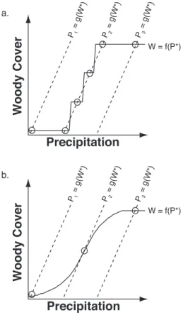
can be directly seen as a proxy for the ability of the vegetated surface to maintain a low albedo, and is therefore linked to a fundamental parameter affecting the climatic state. Woody cover depends on vegetation productivity. In semiarid regions it is limited primarily by the availability of water, and is therefore a function of precipitationP . For

20

a fixed, given amount of precipitationP∗ _{(with the asterisk indicating that the amount}

of precipitation is treated as an independent variable in this case) we can plot a line

W =f (P∗_{) as shown in Fig.}₁_{by the solid lines. A common way to simulate}

vegetation-related properties is to use a biome classification. In such a classification, the vege-tated state may be characterized by a few possible values forW , each representative

25

of the mean value for the respective biome. Consequently, the functional relationship

W =f (P∗_{) is essentially a step function as shown in Fig.}₁_{a. A continuous}

parameteriza-tion forW =f (P∗_{), which would account for a mixture of vegetation types and its diversity}

(6)

BGD

Full Screen / Esc

EGU On the other hand,_{W affects land surface functioning, through land surface}

param-eters such as surface albedo, aerodynamic roughness, and rooting zone depth. These attributes affect the overlying atmosphere, and thereby the rate of precipitation. For a fixed given value ofW∗_{, one can plot the relationship}

P =g(W∗

) for different precipitation regimes, indicated byP1,P2, andP3in Fig.1(dashed lines). The sensitivity of

precip-5

itationP to different values of W∗ _{is represented by the steepness of the curve, with a}

vertical line representing the case of no dependence ofP on W∗_.

Possible solutions to the coupled water- and carbon balances – characterized byP

andW respectively – are given by the intersection of the lines W =f (P ) and P =g(W )

in Fig.1. If this were not the case, the water- and carbon balances would not be in

10

a steady state and would evolve towards one. Imagine a point (W′_{, P}′_{) for which this}

is not the case. IfW′_{>f (P}′_{), then this would imply that either the biomass}_W′ _cannot

be sustained with the given amount of precipitation P′_{, or that a given woody cover}

W′ _{would result in a precipitation rate that is greater than} _P′ _(because _g(W′₎_>P′_{), or}

a combination of both. Consequently, the water- and carbon balances would evolve

15

towards a point (P′′_{, W}′′_{) at which}_W′′

=f (P′′_{) and}_P′′

=g(W′′_).

As we can see from Fig.1, the representation of vegetation by a discrete number of “biome” classes leads to MSS for the precipitation regime indicated byP2, even though

a smooth, continuous representation of vegetation would only lead to one intersection of the curves, and therefore to only one possible steady state. From this conceptual

20

example we can conclude that the way that vegetation is treated in a climate model plays a critical role on whether multiple steady states can emerge from the model dynamics.

Here, we use a coupled dynamic vegetation-atmosphere model of intermediate com-plexity to investigate the role of vegetation classes in the emergence of MSS. To do so,

25

we convert a continuous parameterization that maps vegetation biomass into land sur-face parameters into one of a few discrete classes. A brief description of our model and how we convert a continuous representation of vegetation into discrete classes is described in the next section. In the results section we present the climatic differences

(7)

BGD

Full Screen / Esc

EGU associated with different initial conditions, how these climatic differences depend on

the prescribed number of vegetation classes and discuss how these relate to the two biogeophysical feedback loops discussed above. We close with a brief summary and conclusion.

2 Methods

5

2.1 The Planet Simulator

We use the Planet Simulator Earth system model of intermediate complexity (Lunkeit et al., 2004, Fraedrich et al., 2005a, Fraedrich et al., 2005b). The Planet Simula-tor consists of a low resolution atmospheric general circulation model, a mixed-layer ocean model, a thermodynamic sea-ice model, and a land surface model. The

atmo-10

spheric model consists of a dynamical core and a physical parameterization package of intermediate complexity for unresolved processes. We use the atmospheric model in its T21 resolution (corresponding to approx. 5.625◦

· 5.625◦ longitude/latitude reso-lution) and 5 vertical layers. Over land, a 5 layer heat diffusion model simulates soil temperature, and a “bucket” model simulates soil hydrology. A dynamic global

vegeta-15

tion model (SimBA) simulates the effect of climate on vegetation-affected land surface parameters, such as surface albedo, surface roughness, and the total soil water holding capacity.

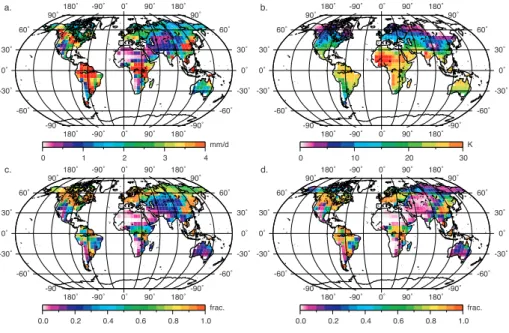
In this study, we use the Planet Simulator in a setup with prescribed sea surface temperatures. The model leads to a reasonable simulated climate and vegetation

dis-20

tribution for present-day forcings (see Fig.2), although some regional deficiencies exist (e.g. dryness of West Africa and central Amazonia). However, for the more conceptual nature of our study, we take this control simulation as being sufficiently suitable for the purpose here. More importantly the dominant climatic effects and feedback mecha-nisms related to differences in vegetation are consistent with those of previous studies

25

(8)

BGD

Full Screen / Esc

EGU 2.2 Discrete versus continuous vegetation classes

The SimBA dynamic vegetation model simulates regional vegetation biomassCvegfrom

the balance of carbon exchange fluxes. Carbon uptake by gross primary productivity GPP depends on incoming photosynthetically active solar radiation, surface tempera-ture, and soil moisture status. Autotrophic respiration is assumed to be 50% of GPP,

5

which is commonly observed and can be understood by optimum nitrogen allocation in canopies (Dewar,1996). Litter production is expressed asCveg/τvegwithτvegbeing

a fixed turnover time. As a consequence, mean vegetation biomass is proportional to mean productivity in our model.

Climatically-relevant land surface parameters are derived from the fractional cover of

10

woody vegetationfw. The woody vegetation cover is derived from vegetation biomass

in the standard version of the model by:

f_w = _c1 c · arctan Cveg− ca c_b ! + cd (1)

In Eq. (1),c_a,c_b,c_c, andc_d are empirical parameters which were derived by matching the resulting distribution of woody vegetation with the observed vegetation distribution.

15

Woody cover is then used to derive, for instance, the soil moisture holding capacity of the rooting zoneWmaxbyWmax=fw · Wmax,veg+(1 − fw) · Wmax,noveg, withWmax,vegbeing

the value for a surface that is completely covered by woody vegetation, andW_max,noveg

being the respective value for a surface in the absence of woody vegetation. Other land surface parameters, specifically leaf area index and leaf cover, surface albedo

20

and roughness, are derived in an analogous way. For details of the vegetation model, seeKleidon(2006a).

In order to introduce discrete vegetation classes, we rewrite f_w in discrete form (which we refer to asf_w,d):

f_w,d = inf(fw· n)

n − 1 (2)

(9)

BGD

Full Screen / Esc

EGU where inf(x) denotes the truncation of the expression x to its integer value, and n is

the specified number of vegetation classes. What Eq. (2) results in is a mapping of biomass to a finite number ofn fractional cover values that then result in a discrete set

of land surface parameters for certain ranges of vegetation biomass. 2.3 Simulation setup

5

We conduct a series of sensitivity simulations which differ by (a) the initialization of the vegetation state (Cveg=0 in a “bare ground” initialization and Cveg=5 kgC m−2in a ”fully

vegetated” initialization) and (b) the number of discrete vegetation classes (n in Eq.2). We use values of_{n= 2, 3, 4, 5, 6, 7, 8, and 10. The continuous vegetation formulation} of Eq.1, which we will refer to asn=∞, is taken as our “Control” simulation.

10

Each sensitivity simulation is run for 40 years. For the first 30 years the time step of the vegetation model is increased in order to accelerate the transition to a steady-state. In this acceleration scheme, we use the time step of the atmospheric model for the first 2 years to allow for the physical climatic variables to come close to a steady-state. For year 3 to 8, we use a factor of 20 to accelerate the carbon pool dynamics, so that the

15

simulated time of 5 years corresponds to 100 years of vegetation dynamics. In the next 5 year intervals, we subsequently decrease the acceleration factor to 10, 5, and 2. During the remaining time, the vegetation model is run at the atmospheric time step. With this setup, we achieve an “effective” simulation period for vegetation dynamics of more than 200 years. With additional sensitivity simulations we confirmed that this

20

acceleration scheme does not affect the outcome of the final steady state (not shown). The motivation for the subsequently decreased time step is that the acceleration of the carbon dynamics also leads to an increase in the variability in the carbon pools. With the decreased acceleration factor in later stages of the simulation, this variability is reduced.

25

We use averages taken over the last 10 years of the simulation period to evaluate the differences in the steady states.

(10)

BGD

Full Screen / Esc

EGU

3 Results and discussion

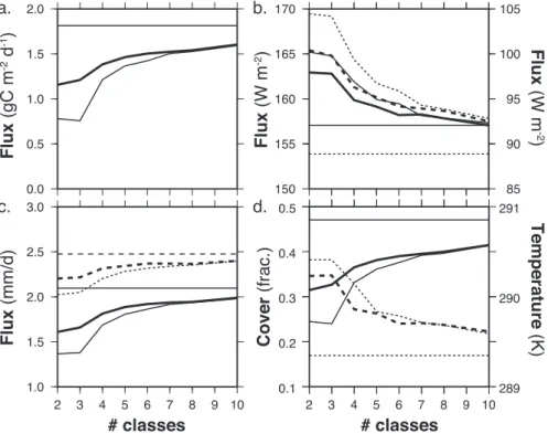
The sensitivity of the land climate to vegetation classes is summarized in Fig.3. These averages show clear differences to the “Control” simulation in simulated vegetation productivity, radiative fluxes, water fluxes, fractional vegetation cover, and near surface air temperature with increasing values of vegetation classesn. The simulations with

5

discrete vegetation classes generally show lower gross primary productivity of 0.8– 1.6 gC m−2_d−1 _{compared to the average value of 1.8 gC m}−2_d−1 _{in the “Control”. In}

terms of the surface energy balance, the net flux of solar and terrestrial radiation is higher by up to 8 W m−2 _{and 16 W m}−2 _{respectively. Precipitation and}

evapotranspi-ration are lower by as much as 0.8 mm d−1 _{and 0.5 mm d}−1 _{respectively. Global land}

10

temperatures show a minor but consistent trend of being warmer by up to ≈1 K. The climatic differences due to initial conditions are generally less than those between the discrete vegetation classification and the ”Control”.

Two general trends can be seen in Fig.3: first, the difference due to the initial condi-tions diminishes with increasing values ofn, and disappears for n=8 or more classes.

15

The other trend is that the steady state climates asymptotically approximate the “Con-trol” climate. However, even after the MSS converge into a single steady state atn=8,

the climate still differs from the “Control”, resulting in climatic conditions that result in lower values of gross primary productivity.

These climatic differences are consistent and can be explained as follows: As

pro-20

ductivity increases with n, so does evapotranspiration and leaf cover. As the land

surface is cooled more effectively by evapotranspiration, the net emission of terres-trial radiation decreases. The increase of evapotranspiration in turn leads to (a) lower surface temperatures due to enhanced latent cooling, (b) enhanced continental pre-cipitation, and (c) increased cloud cover (not shown). The increase in cloud cover

25

results in lower absorption of solar radiation, even though surface albedo decreases with increased leaf cover.

(11)

BGD

Full Screen / Esc

EGU differs due to different initial conditions and different number of vegetation classes. Note

that differences in Cveg represent differences in vegetation productivity, because the

model uses a fixed residence time to simulate biomass (see Sect.2). In the extreme case of n=2, vegetation biomass is substantially reduced compared to the “Control”

across all regions. This reduction is still present in the case of _{n=8, but less}

pro-5

nounced. The differences in biomass due to initial conditions for n=2 can be found in tropical South America, China, western Europe, and North America. The differences in biomass for_{n=8 are comparatively minor.}

These differences in steady state biomass result from differences in the dominant factors that limit productivity. The dominant limitation in the high latitudes is the length

10

of the growing season. The difference in vegetation states affect primarily the amount of absorbed solar radiation in the presence of snow, thereby affecting springtime temper-atures. The differences in northern hemisphere springtime temperatures Tmam(March–

May) are shown in Fig.5. These results show thatTmamis relatively insensitive to initial

conditions forn=2 and n=8. Compared to the “Control”, both cases show large regions

15

in the high latitudes for whichTmamare colder by 2 K and more. These differences

cor-respond well to the differences in biomass shown in Fig.4. This leads us to conclude that the vegetation and climate differences in these regions are primarily caused by the effect of vegetation on snow albedo and growing season length.

The differences in biomass due to initial conditions for n=2 can be attributed primarily

20

to differences in water availability, as shown in the differences in annual mean precip-itation (Fig.6). The locations of higher biomass in Fig.4a correspond well with those of higher precipitation in Fig. 6a. Similarly, differences in biomass compared to the “Control” can generally be attributed to differences in precipitation for tropical regions (and to some extent for temperate regions), and thus linked with the dominant control

25

(12)

BGD

Full Screen / Esc

EGU

4 Conclusions

This paper shows that multiple steady states in the coupled vegetation-atmosphere system can emerge as a result of a discrete representation of vegetation form and function in an Earth system model of intermediate complexity, as hypothesized in Fig.1. The two major positive vegetation feedbacks that result in the emergence of these

5

steady states are related to the temperature limitation on productivity in high latitudes and the water limitation in the tropics and subtropics. This finding is consistent with previous studies.

These results have two important implications for representing vegetation dynamics in Earth system models. First, multiple steady states in the vegetation-atmosphere

10

system may simply be model artefacts that disappear if the full complexity and hetero-geneity in vegetation form and functioning is represented in the model. What this would then imply is that catastrophic regime shifts that are associated when the vegetation-atmosphere system switches from one to another steady state due to some external perturbation are model artefacts and would be unlikely to occur in more complex

rep-15

resentation of vegetation form and functioning. Second, a discrete representation of vegetation as is typically done in dynamic global vegetation models in terms of plant functional types seems to result in a general underestimation of terrestrial productivity. Both of these implications are important to keep in mind when we want to understand the overall response of the terrestrial biosphere to past and future climatic changes.

20

Acknowledgements. This research was initiated as part of the Undergraduate Research

As-sistance Program of the University of Maryland. Funding was provided to A. Kleidon by the NSF climate dynamics program through grant ATM 0513506. KF acknowledges support by DFG-Project FR 450/11-1.

(13)

BGD

Full Screen / Esc

EGU

References

Bonan, G. B., Pollard, D., and Thompson, S. L.: Effects of boreal forest vegetation on global climate, Nature, 359, 716–718, 1992. 689

Brovkin, V., Claussen, M., Petoukhov, V., and Ganopolski, A.: On the stability of the atmosphere-vegetation system in the Sahara/Sahel region, J. Geophys. Res., 103(D24), 5

31 613–31 624, 1998. 690

Brovkin, V., Levis, S., Loutre, M.-F., Crucifix, M., Claussen, M., Ganopolski, A., Kubatzki, C., and Petoukhov, V.: Stability analysis of the climate-vegetation system in the northern high latitudes, Clim. Ch., 57, 119–138, 2003. 689

Budyko, M. I.: The Effect of Solar Radiation Variations on the Climate of the Earth, Tellus, 21, 10

611–619, 1969. 689

Charney, J. G.: Dynamics of deserts and drought in the Sahel, Quart. J. Roy. Meteorol. Soc., 101, 193–202, 1975. 690

Claussen, M.: On coupling global biome models with climate models, Clim. Res., 4, 203–221, 1994. 689,690

15

Claussen, M.: Modeling bio-geophysical feedback in the African and Indian monsoon region, Clim. Dyn., 13, 247–257, 1997. 690

Claussen, M.: On multiple solutions of the atmosphere-vegetation system in present-day cli-mate, Glob. Ch. Biol., 4, 549–559, 1998. 690

Dewar, R. C.: The correlation between plant growth and intercepted radiation: an interpretation 20

in terms of optimal plant nitrogen content, Ann. Bot., 78, 125–136, 1996. 693

Fraedrich, K.: Catastrophes and resilience of a zero-dimensional climate system with ice-albedo and greenhouse feedback, Quart. J. Roy. Meteorol. Soc., 105, 147–167, 1979.689

Fraedrich, K., Jansen, H., Kirk, E., Luksch, U., and Lunkeit, F.: The Planet Simulator: Towards a user friendly model, Z. Meteorol., 14, 299–304, 2005a. 692

25

Fraedrich, K., Jansen, H., Kirk, E., and Lunkeit, F.: The Planet Simulator: Green planet and desert world, Z. Meteorol., 14, 305–314, 2005b. 692

Harvey, L. D. D.: On the role of high latitude ice, snow, and vegetation feedbacks in the climatic response to external forcing changes, Climatic Change, 13, 191–224, 1988. 689

Kleidon, A.: The climate sensitivity to human appropriation of vegetation productivity and its 30

thermodynamic characterization, Glob. Planet. Ch., 54, 109–127, 2006a. 692,693

(14)

BGD

Full Screen / Esc

EGU

with climate model simulations, Biologia, Bratislava, 61/Suppl. 19, S234–239, 2006b.692

Kleidon, A. and Fraedrich, K.: Biotic Entropy Production and Global Atmosphere-Biosphere In-teractions, in Non-Equilibrium Thermodynamics and the Production of Entropy: Life, Earth, and Beyond, edited by: A., and Lorenz, R. D., 173–190, Springer Verlag, Heidelberg, Ger-many, 2005.689

5

Levis, S., Foley, J. A., Brovkin, V., and Pollard, D.: On the stability of the high-latitude climate-vegetation system in a coupled atmosphere-biosphere model, Glob. Ecol. Biogeog., 8, 489– 500, 1999.689

Lunkeit, F., Fraedrich, K., Jansen, H., Kirk, E., Kleidon, A., and Luksch, U.: Planet Simulator Reference Manual, available athttp://puma.dkrz.de/plasim, 2004. 692

10

Otterman, J., Chou, M. D., and Arking, A.: Effects of nontropical forest cover on climate, J. Clim. Appl. Meteorol., 23, 762–767, 1984.689

Pielke, R. A., Schimel, D. S., Lee, T. J., Kittel, T. G. F., and Zeng, X.: Atmosphere-terrestrial ecosystem interactions: implications for coupled modeling, Ecol. Modell., 67, 5–18, 1993.

689

15

Sellers, W. D.: A Global Climatic Model Based on the Energy Balance of the Earth-Atmosphere System, J. Appl. Meteorol., 8, 392–400, 1969.689

Wang, G.: A conceptual modeling study on biosphere-atmosphere interactions and its implica-tions for physically based climate modeling, J. Clim., 17, 2572–2583, 2004.690

Wang, G. and Eltahir, E. A. B.: Biosphere-atmosphere interactions over West Africa. 2. Multiple 20

climate equilibria, Quart. J. Roy. Meteorol. Soc., 126, 1261–1280, 2000a. 690

Wang, G. and Eltahir, E. A. B.: Ecosystem dynamics and the Sahel drought, Geophys. Res. Lett., 27, 795–798, 2000b. 690

Zeng, N. and Neelin, J. D.: The role of vegetation-climate interaction and interannual variability in shaping the African savanna, J. Clim., 13, 2665–2670, 2000. 690

25

Zeng, X., Shen, S. S. P., Zeng, X., and Dickinson, R. E.: Multiple equilibrium states and the abrupt transitions in a dynamical system of soil water interacting with vegetation, Geophys. Res. Lett., 31, L05501, doi:10.1029/2003GL018910, 2004. 690

(15)

BGD

Full Screen / Esc

Printer-friendly Version Interactive Discussion EGU Woody Cover Precipitation W = f(P*) P = g(W*)1 P = g(W*)2 P = g(W*)3 Woody Cover Precipitation W = f(P*) P = g(W*)1 P = g(W*)2 P = g(W*)3 a. b.

Fig. 1. Conceptual diagram to illustrate the effect of vegetation parameterizations on the

emergence of multiple steady states. Diagram (a) shows the case in which vegetation is pa-rameterized by a few discrete vegetation classes while (b) uses a continuous representation of vegetation. The solid lines represent woody vegetation coverW =f (P∗_{) as a function of a fixed,}

given value of precipitationP∗_{. The dashed lines represent precipitation}_{P =g(W}∗_{) as a function}

(16)

BGD

Full Screen / Esc

Printer-friendly Version Interactive Discussion EGU c. d. a. b. 180˚ 180˚ -90˚ -90˚ 0˚ 0˚ 90˚ 90˚ 180˚ 180˚ -90˚ -90˚ -60˚ -60˚ -30˚ -30˚ 0˚ 0˚ 30˚ 30˚ 60˚ 60˚ 90˚ 90˚ 0.0 0.2 0.4 0.6 0.8 1.0 frac. 180˚ 180˚ -90˚ -90˚ 0˚ 0˚ 90˚ 90˚ 180˚ 180˚ -90˚ -90˚ -60˚ -60˚ -30˚ -30˚ 0˚ 0˚ 30˚ 30˚ 60˚ 60˚ 90˚ 90˚ 0.0 0.2 0.4 0.6 0.8 1.0 frac. 180˚ 180˚ -90˚ -90˚ 0˚ 0˚ 90˚ 90˚ 180˚ 180˚ -90˚ -90˚ -60˚ -60˚ -30˚ -30˚ 0˚ 0˚ 30˚ 30˚ 60˚ 60˚ 90˚ 90˚ 0 1 2 3 4 mm/d 180˚ 180˚ -90˚ -90˚ 0˚ 0˚ 90˚ 90˚ 180˚ 180˚ -90˚ -90˚ -60˚ -60˚ -30˚ -30˚ 0˚ 0˚ 30˚ 30˚ 60˚ 60˚ 90˚ 90˚ 0 10 20 30 K

Fig. 2. Simulated climate of the control setup of the Planet Simulator in T21L5 setup. The

graphs show annual means of (a) precipitation; (b) near surface air temperature; (c) leaf cover; and (d) woody cover.

(17)

BGD

Full Screen / Esc

Printer-friendly Version Interactive Discussion EGU 0.1 0.2 0.3 0.4 0.5 1.0 1.5 2.0 2.5 3.0 Flux (mm/d) 2 3 4 5 6 7 8 9 10 # classes Cover (frac.) 2 3 4 5 6 7 8 9 10 # classes 0.0 0.5 1.0 1.5 2.0 Flux (gC m -2 d -1 ) 150 155 160 165 170 Flux (W m -2 ) 85 90 95 100 105 Flux (W m -2 ) a. b. c. d. 289 290 291 Temperature (K)

Fig. 3. Climate sensitivity of annual mean land averages of (a) gross primary productivity,

(b)net solar (solid line, left scale) and terrestrial (dashed line, right scale, positive = radiative cooling) radiation at the surface, (c) evapotranspiration (solid) and precipitation (dashed), and

(d)fractional cover (solid) and near surface air temperature (dashed) to the number of vege-tation classesn. The thick (thin) lines show the sensitivity for the initialization of fully (bare)

woody vegetation cover respectively. The horizontal lines indicate the respective values of the “Control” simulation.

(18)

BGD

Full Screen / Esc

Printer-friendly Version Interactive Discussion EGU c. d. a. b. 180° 180° -90° -90° 0° 0° 90° 90° 180° 180° -90° -90° -60° -60° -30° _-30° 0° _0° 30° 30° 60° 60° 90° 90° -2 -1 0 1 2 kgC m-2 180° 180° -90° -90° 0° 0° 90° 90° 180° -90° -90° -60° -60° -30° 0° 30° 60° 60° 90° 90° -2 -1 0 1 2 kgC m-2 180° -90° 0° 90° 180° -90° -90° -60° -60° -30° -30° 0° _0° 30° 30° 60° 60° 90° 90° 180° -90° 0° 90° 180° 180° -90° -90° -60° -60° -30° 0° 30° 60° 60° 90° 90°

Fig. 4. Climatic differences in vegetation biomass for (a) “full vegetation” – “bare ground” for

n=2 (b) same as (a), but for “full vegetation” – “Control”, (c) and (d) are the same as (a) and

(19)

BGD

Full Screen / Esc

Printer-friendly Version Interactive Discussion EGU c. d. a. b. 180° 180° -90° -90° 0° 0° 90° 90° 180° 180° -90° -90° -60° -60° -30° -30° 0° 0° 30° _30° 60° 60° 90° 90° -2 -1 0 1 2 K 180° 180° -90° -90° 0° 0° 90° 90° 180° -90° -90° -60° -60° -30° 0° 30° 60° 60° 90° 90° -2 -1 0 1 2 K 180° -90° 0° 90° 180° -90° -90° -60° -60° -30° -30° 0° _0° 30° _30° 60° 60° 90° 90° 180° -90° 0° 90° 180° 180° -90° -90° -60° -60° -30° 0° 30° 60° 60° 90° 90°

Fig. 5. Same as Fig. 4, but for northern hemisphere springtime (March–May) near surface air

(20)

BGD

Full Screen / Esc

Printer-friendly Version Interactive Discussion EGU c. d. a. b. 180° 180° -90° -90° 0° 0° 90° 90° 180° 180° -90° -90° -60° -60° -30° _-30° 0° 0° 30° 30° 60° 60° 90° 90° -2 -1 0 1 2 mm/d 180° 180° -90° -90° 0° 0° 90° 90° 180° -90° -90° -60° -60° -30° 0° 30° 60° 60° 90° 90° -2 -1 0 1 2 mm/d 180° -90° 0° 90° 180° -90° -90° -60° -60° -30° -30° 0° 0° 30° _30° 60° 60° 90° 90° 180° -90° 0° 90° 180° 180° -90° -90° -60° -60° -30° 0° 30° 60° 60° 90° 90°