The development of more effective operating plans for bus service

The Development of More Effective Operating Plans for Bus Service

by

Yoosun Hong

B.S., Urban Planning and Engineering

Yonsei University, 2000

Submitted to the Department of Civil and Environmental Engineering

In Partial Fulfillment of the Requirements of the Degree of

Master of Science in Transportation

at the

Massachusetts Institute of Technology

September 2002

BARKER

SEP

_{1 9 2002}

LIBRARIES

0 2002 Massachusetts Institute of Technology

All rights Reserved

Signature of Author... -....

Department of Civil and Environmental Engineering

August 23, 2002

Certified

by ...

...

-

-/

Accepted

by ...

Professor Nigel H.M. Wilson

Thesis Supervisor

The Development of More Effective Operating Plans for Bus Services

by

Yoosun Hong

Submitted to the Department of Civil and Environmental Engineering on August 23, 2002 in Partial Fulfillment of the Requirements of the

Degree of Master of Science in Transportation

Abstract

This thesis develops relationships between schedule parameters, operational cost, and service quality involved in the scheduling process, which will help a decision-maker to choose the schedule that best fits his or her objectives. It also proposes a scheduling process, which incorporates the developed relationships and enables schedulers to explore different combinations of schedule parameters. The developed relationships are demonstrated and the proposed scheduling process is applied in a case study of the Chicago Transit Authority bus route 77.

The trip time distribution changes depending on the headway and the schedule time since the headway and schedule time affects the dwell time and movement time respectively which are components of the vehicle trip time. The half cycle time and recovery time are determined by the desired on-time departure probability at the terminal and the trip time distribution that is determined by the schedule time and headway. Therefore, any changes in the headway and schedule time will influence decisions on other schedule parameters.

The operational cost includes both the schedule cost and cost of any late trip. The schedule cost during a time period is determined by the cycle time and headway and the late trip cost is determined by the trip time distribution and cycle time. The service quality is measured by the in-vehicle time, crowding level, passenger waiting time, and schedule adherence. The in-vehicle time is affected by the headway and schedule time, the waiting time and crowding level are affected by vehicle headway and recovery time, and the schedule adherence is affected by the

schedule time and recovery time.

The case study showed that understanding and applying those relationships to the proposed scheduling process can help transit agencies develop more effective operations plans by recognizing the tradeoffs between the schedule parameters, operational cost and service quality. The recommended schedule parameters under the current headway resulting from the proposed scheduling process could significantly reduce operational costs while improving the passenger waiting time and on time arrival probability compared to the current schedule.

Thesis Supervisor: Nigel H.M. Wilson

Acknowledgement

I would like to express my deep gratitude to my supervisor, Professor Nigel H. M.

Wilson for his guidance and encouragement during the course of this research. His advice, and patience were invaluable to me. I am also indebted to Harilaos Koutsopoulos at the Volpe Center

for his thorough feedback and advice which help improve my research a lot.

I would like to thank my friends in MIT for sharing in all my joys and sorrows with me.

Without them, my life in MIT would not have been enjoyable. I wish them the best of luck in the future.

Finally, I would like to thank my parents and family in Korea who has supported me throughout my life. Without their support and encouragement, I could not have been where I am today.

Table of Contents Abstract ... .. 3 Acknowledgements ... ... 5 Table of Contents ... 7 List of Figures ... ...- 9 List of Tables ... ... 10 Chapter 1. Introduction 11 1.1. Motivation 11 1.2. Objectives 13 1.3. Literature Review 13 1.4. Research Approach 15 1.5. Thesis Organization 16

Chapter 2. Bus Operations Planning 17

2.1. Operations Planning Overview 17

2.1.1. Network Design 18

2.1.2. Service Frequency/Span Setting 19

2.1.3. Timetable Development 19

2.1.4. Vehicle Scheduling 20

2.1.5. Crew Scheduling 20

2.2. Schedule Parameters in Operations Plan 21

Chapter 3. Theoretical Analysis of Relationships between Schedule Parameters.

Operational Cost, and Service Ouality 26

3.1. Route Description and Basic Assumption 26

3.2. Trip Time Distribution and Schedule Parameters 28

3.2.1. The Influence of Time Points and Schedule Time on Trip Time 28

3.2.2. Setting Cycle Time and Recovery Time 38

3.2.3. Dwell Time 39

3.3. Relationships between Schedule Parameters 44

3.3.1. Schedule Time and Recovery Time 44

3.3.2. Recovery Time and Vehicle Headway 46

3.4. Operational Cost and Schedule Parameters 49

3.4.1. Cost Model 49

3.4.2. Operational Cost and Cycle Time 51

3.4.3. Operational Cost and Vehicle Headway 52

3.4.4. Vehicle Headway and Cycle Time 52

3.5. Service Quality and Schedule Parameters 53

3.5.1. Passenger In-vehicle Time 53

3.5.2. Passenger Waiting Time 53

3.5.3. Schedule Adherence 55

3.5.4. Crowding 55

Chapter 4. CTA Route 77 Application 59

4.1. Route 77 Characteristics 59

4.1.1. Route Description 59

4.1.2. Current Timetable 61

4.2. AVL and AFC Systems Data Analysis 63

4.2.1. Data 63

4.2.2. Trip Time Analysis 64

4.2.3. Passenger Demand Analysis 68

4.3. Trip Time Distribution and Dwell Time Model Estimation 69

4.3.1. Trip Time Distribution Estimation 70

4.3.2. Dwell Time Model Estimation 74

4.4. Relationships Estimation 78

4.4.1. Trip Time Distribution and Schedule Time 79

4.4.2. Trip Time Distribution and Headway 83

4.5. Operational Cost and Service Quality Estimation 85

4.5.1. Operational Cost Estimation 86

4.5.2. Service Quality Estimation 87

4.6. Applying Scheduling Process 88

4.7. Case Evaluations 91

4.7.1. Case 1: Current Headway 91

4.7.2. Case 2: Increased Headway 97

4.7.3. Case 3: Decreased Headway 101

4.7.4. Headway Recommendation 104

4.7.5. Discussion 106

Chapter 5. Summary and Conclusions 108

5.1. Summary 108

List of Figures

Figure 2-1 Service and Operations Planning Hierarchy... 18

Figure 2-2 Inter-relationships between Schedule Parameters ... 23

Figure 2-3 The Relationship between Operational Cost and Schedule Parameters ... 24

Figure 2-4 The Relationship between Service Quality and Schedule Parameters ... 25

Figure 3-1 A Route with k Possible Time Points ... 27

Figure 3-2 Unconstrained Trip Time Distribution... 29

Figure 3-3 Route with One Tim e Point ... 31

Figure 3-4 Trip Time Distribution with Different Schedule Trip Times ... 35

Figure 3-5 Trip Time Distribution with Different Number of Time Points... 36

Figure 3-6 Influence of the Location and Schedule Time of the Last Time Point ... 37

Figure 3-7 Probability and Cumulative Distributions ... 38

Figure 3-8 Cumulative Distribution with Different Schedule Times ... 44

Figure 3-9 Relationship between Scheduled Trip Time and Recovery Time ... 46

Figure 3-10 Departure Headway Distribution at Terminal with Different Recovery Times... 48

Figure 4-1 CTA Route 77, Belm ont... 60

Figure 4-2 Recovery Time for Route 77 ... 62

Figure 4-3 Eastbound Scheduled Headway (between Central and Halsted)...63

Figure 4-4 Eastbound Scheduled and Actual Trip Time...65

Figure 4-5 Westbound Scheduled and Actual Trip Time... 65

Figure 4-6 Eastbound Dw ell Tim e ... 66

Figure 4-7 W estbound Dw ell Tim e... 67

Figure 4-8 Eastbound M ovement Time... 67

Figure 4-9 Westbound Movement Time ... 68

Figure 4-10 Passenger Arrival Rate ... 69

Figure 4-11 Eastbound Probability Distribution... 72

Figure 4-12 Westbound Probability Distribution ... 73

Figure 4-13 Eastbound Cumulative Probability Distribution... 73

Figure 4-14 Westbound Cumulative Probability Distribution ... 74

Figure 4-15 Relationship between Total Dwell Time and Passenger Demand (Eastbound)... 75

Figure 4-16 Relationship between Total Dwell Time and Passenger Demand (Westbound)...75

Figure 4-17 Eastbound Trip Time Distributions with Different Schedule Times... 80

Figure 4-18 Westbound Trip Time Distributions with Different Schedule Times ... 81

Figure 4-19 Relationship between Schedule Time and Recovery Time (Westbound)...82

Figure 4-20 Eastbound Trip Time Distributions with Different Headways ... 85

Figure 4-21 Westbound Trip Time Distributions with Different Headways ... 85

Figure 4-22 Relationship between Schedule Time, On Time Arrival Probability and In-vehicle T im e ... ... . ---... 9 3 Figure 4-23 Tradeoff between In-vehicle Time and Waiting Time... 93

Figure 4-24 Relationship between Cycle Time and Operational Cost ... 94

Figure 4-25 Eastbound Trip Time Distributions (6 minutes headway) ... 98

Figure 4-26 Westbound Trip Time Distributions (7 minutes headway)... 98

Figure 4-27 Eastbound Trip Time Distribution (4 minutes headway)... 101

Figure 4-28 Westbound Trip Time Distributions (5 minutes headway)... 102

List of Tables

Table 3-1 Holding Points Locations with Different Number of Time Points ... 35

Table 3-2 Cumulative Probability of Trip Times ... 39

Table 3-3 Probability of Trip Times with Different Scheduled Trip Times ... 45

Table 4-1 Schedule Tim e for Route 77 ... 61

Table 4-2 Trip Time statistics by Time Period ... 64

Table 4-3 Movement and Dwell Times Statistics... 66

Table 4-4 Statistics of Trip Times of Sub-time Periods during AM peak ... 71

Table 4-5 Statistics of Trip Tim es... 72

Table 4-6 Eastbound Schedule Parameters in minutes ... 81

Table 4-7 Westbound Schedule Parameters in minutes ... 81

Table 4-8 Changed Schedule Parameters with Minimum Recovery Time... 83

Table 4-9 Passenger Demand and Dwell Time ... 84

Table 4-10 Passenger Demand and Dwell Time with Changed Headway ... 84

Table 4-11 A ssessm ent Cases ... 90

Table 4-12 Schedule Parameters in minutes (Current Headway)... 91

Table 4-13 Operational Cost and Service Quality with Current Headway... 92

Table 4-14 In-vehicle Time and Waiting Time Changes with Current Headway... 94

Table 4-15 Number of buses needed with Current Headway... 96

Table 4-16 Current Schedule Parameters, Service Quality, and Operational Cost ... 97

Table 4-17 Schedule Parameters in minutes (Increased headway)... 99

Table 4-18 Operational Cost and Service Quality with Increased Headway ... 99

Table 4-19 In-vehicle Time and Waiting Time Changes with Increased Headway... 100

Table 4-20 Number of buses needed with Increased Headway... 100

Table 4-21 Schedule Parameters in minutes (Decreased headway) ... 102

Table 4-22 Operational Cost and Service Quality with Decreased Headway... 103

Table 4-23 In-vehicle Time and Waiting Time Changes with Decreased Headway ... 103

Table 4-24 Number of buses needed with Decreased Headway ... 104

Chapter 1. Introduction

This thesis develops relationships between schedule parameters, operational cost, and service quality involved in the scheduling process. The developed relationships are demonstrated through application to a specific bus route. The application shows that understanding and applying those relationships to the scheduling process can help transit agencies develop more effective operations plans.

1.1.

Motivation

Maintaining transit service reliability has long been a major concern of both transit operators and users. Failure to maintain transit service reliability results in late departures, bunching, crowding and missed trips. Transit operators will have to bear higher operating costs and purchase additional vehicles to solve these problems. Unreliable service increases passenger wait times and levels of crowding, and thus discourages potential customers from using transit. This translates into lost revenue as well as ridership for the transit agencies. Thus, transit operators have long been interested in finding means to improve service reliability. Research on improving service reliability on bus routes is especially important since bus routes are vulnerable to traffic congestion because buses share the road with other traffic unlike trains, which usually have their own right of way.

Fortunately, with the development over the past two decades of Intelligent Transportation System (ITS), Automatic Vehicle Location (AVL) and Automatic Fare Collection (AFC) systems more detailed information can be obtained on running times and passenger demand than with traditional manual data collection. This enables faster and more accurate data analysis and service performance evaluation under the current timetable, and therefore more rapid adjustment of the timetable. However, in reality, most transit providers cannot readily utilize the data gained from existing AVL and AFC systems for off-line analysis and in the scheduling process even if they have made large investments in AVL systems. Therefore, research is needed to utilize those data more efficiently in the scheduling process and to estimate the benefit of more accurate information on running time and passenger demand in terms of developing more effective timetables.

Developing a timetable involves different objectives. Passengers are interested in minimizing their waiting time and riding time, and thus prefer short scheduled running time, high frequency and high reliability. They are also concerned about crowding levels, which again makes them prefer high frequency and high reliability. The operator is interested in minimizing operating costs, and thus prefers short running time, minimum frequency and minimum recovery time (although they want recovery time to be sufficient that most return trips can begin on time). However, high reliability and short scheduled running times are in conflict since the probability that a driver stays on schedule decreases as the schedule becomes tighter (i.e. the schedule running time become shorter). Therefore, service reliability deteriorates. In addition, the optimal schedule for the passengers is not necessarily optimal for the operator. Thus, a transit operator should make decisions on the tradeoffs between operating costs and passenger level of service when setting a timetable. Therefore, it will be helpful for transit agencies to better understand the relationships between schedule parameters (schedule time, necessary recovery time, and frequency) and operating cost and passenger service level in choosing the timetable that would be optimal for their objectives.

Implementation of operations control strategies presents a further complication. Operational control strategies such as holding and signal priority treatment directly change the mean and variability of running time, which are critical in setting the scheduled running time and necessary recovery time. Therefore a schedule that is optimal without operational controls may not be optimal when operational controls are applied on a route. For example, if a holding strategy is implemented on a route, longer schedule running time and shorter recovery time than before will be needed due to increased running time and on-time performance (in terms of improvement of speed and reliability). Therefore, research is needed to help find the combination of schedule parameters (schedule time, recovery time, and frequency) that meets operator and passenger objectives when operations control strategies are implemented.

1.2.

Objectives

The principal objectives of this research are therefore:

1) to understand the relationships between schedule parameters, operational cost, passenger demand, and service quality.

2) to develop a process for selecting the schedule parameters and apply it to a specific bus route.

3) to demonstrate how these relationships affect the timetable setting process through

application to a specific bus route.

1.3.

Literature Review

Muller and Furth (2000) show how service planning can be integrated with operational control using simple illustrations based on the system implemented in Eindhoven, the Netherlands. First, they present the impact of operations control on improving service quality. In their research, they use holding strategy at time points and conditional traffic signal priority at signalized intersections as operations control strategies. They found that these operations control strategies do indeed help reduce schedule deviation, thus reducing passenger wait time. This research also shows the way that data gathered using on-board computers can be analyzed and used to help create a better schedule. TRITAPT (TRIp Time Analysis for Public Transport) is used for data analysis and to plan the schedule. Finally, they show the improvement in service performance which can be achieved by integrating operations planning and operations control. This research resulted in a feasible schedule which trades off speed and schedule variation.

Wirasinghe and Liu also studied transit route schedule design in their papers. In the paper, Optimal Schedule Design for a Transit Route with One Intermediate Time Point (1995), they showed that the decisions on the number and locations of time points and the scheduled travel times between adjacent time points are important in schedule design for a route. The optimal amount of slack time and whether the time point is necessary are determined by minimizing the expected total cost, which consist of operating cost, passenger waiting cost, and delay cost. In this paper, they found out that the optimal design of a schedule is sensitive to the passenger demand pattern along the route and that a time point is needed only when the number of boarding passengers is much larger than the number of through passengers. They also developed a simulation model of schedule design for a fixed transit route using the holding

at each time point can be determined using the simulation model by minimizing total cost associated with the schedule. They demonstrated the potential savings from the model through application to a route of Calgary Transit.

There have also been several efforts to develop dwell time models. In general, these have used ordinary least squares regression to derive the dwell time as a function of the numbers of passengers boarding and alighting and other operating characteristics such as fare payment method, seat availability, and number of doors used for boarding and alighting. Lin and Wilson

(1993), in their dwell time relationships analysis, developed dwell time models for one-car and

two-car light rail operations. The result of those models showed that the number of passengers boarding and alighting and passenger "friction" caused by the passengers already on board significantly affects the dwell time. Several forms of passenger friction term based on the number of standees, were tested and proved to significantly affect the dwell time. Aashtiani and Iravani (2002) developed various dwell time models as a function of passenger volume, which were used in the City of Tehran transit assignment model. Two types of models are considered in their research: one is a disaggregate model which attempts to estimate the dwell time at each stop and the other is an aggregate model which attempts to estimate the total dwell time for all the stops on the route. Number of passengers boarding and alighting, load factor, and some bus characteristics such as capacity and number of doors were considered as variables which may influence the dwell time.

Furth (1980) reviewed both practical and theoretical approaches to set the service frequency and developed a model to solve this problem. The model assigned the available vehicles between time periods and between routes so as to maximize the benefit under constraints on subsidy, fleet size and levels of vehicle loading. He showed that this problem can be formulated either as a fixed demand minimization of total expected passenger waiting time or as a variable demand consumer surplus maximization with very similar results. Koutsopoulos (1983) also formulated the problem of setting frequency as a nonlinear mathematical program with the objective of minimizing the social cost including passenger waiting times, crowding levels, and operational costs under constraints on the fleet size, vehicle capacity, and subsidy.

Some of the previous research reviewed is similar to the proposed research in that it dealt with the impacts of decisions on specific schedule parameters on various costs. In general, they tried to find an optimal value for a schedule parameter by minimizing the total cost when other

schedule parameters were fixed. Wirasinghe and Liu studied the impacts of schedule time and Furth and Koutsopoulous studied those of frequency. By developing different forms of dwell time models, the relationship between passenger demand and dwell time has been studied which leads to the relationship between frequency and dwell time.

This research considered the decision on each schedule parameter independently. Therefore, they tried to optimize the specific schedule parameter based on the schedule parameters determined at the previous steps being a fixed input at the current step. So, the full set of relationships between schedule parameters have not been considered. However, schedule parameters affect the operational cost and passenger service levels, and furthermore changes in one schedule parameter can influence decisions on other schedule parameters. Therefore, it is important to understand the possible impacts of schedule parameter change as well as the general relationships between schedule parameters, operational cost and service quality. In this research,

I will develop the relationships between schedule parameters, service quality and operational cost

and also develop an effective scheduling process, which enable the schedule parameters to interact with each other and thus enable the transit operator to find combinations of schedule parameters which better meet their objective.

1.4.

Research Approach

The primary goal of this thesis is to understand the relationships between schedule parameters, operational cost, and service quality that can help transit agencies in developing more effective timetables. The relationships are developed from an analytical model of a simplified bus route incorporating a holding strategy at time points. First, an analytical model to estimate the trip time distribution with different scheduled departure times at the time points and different numbers of time points is developed. And a dwell time model is built to assess the impact of headway changes on the trip time distribution. Second, the impacts of changes in the trip time distribution caused by the change of one scheduled parameter on the other scheduled parameters are explored. Third, the relationships between the operational cost and the schedule parameters are derived by developing a cost model, which is a function of the schedule parameters. Finally, the impacts on service quality of possible changes in the scheduled parameters are estimated.

to the scheduling process of a specific bus route. In order to estimate the trip time distribution changes resulting from schedule time and headway changes, the trip time estimation model and the dwell time model developed in the theoretical analysis are estimated and applied. The case study will also show the tradeoff between the operational cost and service quality when different combinations of schedule parameters are chosen.

1.5.

Thesis Organization

This thesis is organized into five chapters. Chapter Two provides a general introduction to operations planning and definitions of schedule parameters, operational cost, and service quality. The inter relationships existing in the schedule parameter setting process are also discussed. Chapter Three develops the theoretical relationship models, which exist between the schedule parameters, operational cost, and service quality. A scheduling process to incorporate these relationships is proposed. Chapter Four presents the case study of CTA route 77, Belmont. The general theoretical relationship models are applied to the scheduling process of CTA route 77 during the AM peak and the tradeoffs between operational cost and service quality with different combinations of schedule parameters are estimated and presented. Chapter Five summarizes and discusses the findings and makes recommendations for future research.

Chapter 2. Bus Operations Planning

This chapter describes the typical operations planning process and defines the key parameters which are established in this process. Section 2.1 gives an overview of service and operations planning. The research focuses primarily on the analysis of relationships involved in setting schedule parameters for a single bus route. Since setting the schedule parameters is at the heart of the vehicle and crew scheduling processes, these decisions largely determine both the costs to the transit agency and the service quality to the passengers. In section 2.2, the definitions of schedule parameters, operational cost, and service quality that will be used in this research are provided and the relationships between them that should be considered in the process of setting the scheduling parameters are discussed.

2.1.

Operations Planning Overview

Designing a transit service involves a series of decisions, which are illustrated in Figure 2-1. The main stages in the planning process are designing the network, setting service frequency and span, developing the timetable, scheduling vehicles and scheduling crews. Typically these steps are solved sequentially with each decision being made based on the decisions made in the previous steps. The planning process can also be divided into service planning and operations planning. Network and route design, service frequency setting, and timetable development are included in the service planning process and vehicle and crew scheduling are included in the operations planning process.

In the network design step, given the demand characteristics, infrastructure, resources and coverage policies, a set of routes is determined. Next, service frequencies by time of the day and service span of each route are decided according to demand characteristics, available vehicles, available budget, and headway and passenger load policies. In the step of developing a timetable, based on the route travel time data and service policies related to service quality, the schedule time and recovery time are set. In the vehicle scheduling step, given a timetable, vehicle blocks (a sequence of revenue and non-revenue activities for each vehicle) covering all trips are scheduled. Given the vehicle scheduling outputs, which are the set of vehicle blocks, crews runs are developed each consisting of several pieces of work from one or more vehicle blocks.

Input Demand Characteristics Infrastructure Resource Service Policies/Standard Demand Characteristics Available Vehicles Available Budget Service Policies/Standard

Route Travel Time Demand Characteristics Service Policies/Standard

Route Travel Time Resource Service Policies/Standard Work Rules Pay Provision Resource Service Policies/Standard Process Network and Route Design Service Frequency/Span Setting

-+

Service Span of each route

Trip Departure

I

on each route

Revenue and Non-revenue Activities by Vehicle

Figure 2-1 Service and Operations Planning Hierarchy

As shown in Figure 2-1, there are service standards and/or policies involved in decision-making at each step of the transit service planning process. These service standards and policies are designed to provide a balance between optimal cost efficiency, which is the interest of transit agencies, and the provision of adequate service to the public, which is the interest of passengers. The next five sections summarize the typical service and operations planning process and the role that service standards and policies play. This discussion is based on the TCRP Report 30, Transit Scheduling: Basic and Advanced Manual (1998).

2.1.1. Network Design

Route design is basically the definition of where each route goes. Again, service policies and standards generally dictate the type of balance between cost efficiency and service to the public in designing the network. The following are usually considered as the basics of network design standards: population density, employment density, spacing between routes/corridors, limits on the number of deviations or branches, and coverage. Network and route design

Timetable Development Crew Duties Vehicle Scheduling Crew Scheduling

typically evolve very slowly over time, partly because of the difficulty of the network design process and partly because agencies are often reluctant to change existing routes for fear of alienating current riders. Network re-design is undertaken only rarely and often only when major capital investments necessitate it.

2.1.2. Service Frequency/Span Setting

The span of service is the duration of time that vehicles provide passenger service on a route. It is measured from the time of the first trip on the route to the time of the last trip on that route. It is also often established by service policies and standards influenced by the demand for services.

The route frequency defines the headway, the time interval between two consecutive revenue vehicles operating in the same direction on a route. It is determined either by policy or

by demand as reflected in factors such as the maximum passenger load. For this purpose, a

maximum load point is defined as the location along a route where the greatest number of passengers are on board. With data on maximum load point counts, the scheduler can determine the number of vehicles that are needed to accommodate the passengers wanting to use the service

given maximum acceptable passenger loads per vehicle.

The demand-based headway is determined based on the maximum load point counts, vehicle capacities, and loading standard, which indicates how many people can be on board at certain times and on certain vehicles. The load standard is expressed as the ratio of passengers allowed on the vehicle to the actual seating capacity of the vehicle expressed as a percentage. If demand is very low then a policy-based headway is set based on the minimum level of service on the route as reflected in the service standard.

2.1.3. Timetable Development

Developing a timetable involves setting the schedule time on a route given the headway determined in the frequency setting step based on the data (trip time, passenger demand, etc) and constraints (number of buses available, subsidy available, etc). Trips are generated based on the selected schedule parameters (frequency and schedule time). The timetable indicates all the times

Schedule time is the number of scheduled minutes assigned to a revenue vehicle to move from one time point to the next with time points being locations along the route, with posted bus arrival (or departure) times. Major intersections that are widely recognized and have good pedestrian access are usually selected as time points. These points usually have high levels of passenger demand. Usually, the schedule time is set to the average running time between time points.

2.1.4. Vehicle Scheduling

Vehicle scheduling is the process of assigning vehicles to the trips generated in the timetable development process. A series of trips is assigned to a single vehicle and is called a "vehicle block." The objective of the vehicle scheduling step is to define vehicle blocks (a sequence of revenue and non-revenue activities for each vehicle) covering all trips so as to minimize fleet size and non-revenue vehicle time under the constraint of minimum and maximum vehicle block length. The agency policies that have the greatest impact on the vehicle scheduling process are recovery time and interlining policies and constraints.

For many agencies, on some or all routes, the amount of recovery time is often determined either by labor agreement or agency policy. These agreements or policies dictate a minimum number of minutes that must be built into the schedule for recovery time. Usually, the minimum recovery time is set to a certain percent of route trip time and many transit agencies use a minimum recovery time of 10 percent of round trip time.

The cycle time is the number of minutes needed to make a round trip on the route, including recovery time. Minimum cycle time is the number of minutes scheduled for the vehicle to make a round trip, including a minimum recovery time.

2.1.5. Crew Scheduling

Crew scheduling is the process of defining crew assignments. First, runs are assembled or cut from the vehicle blocks generated in the vehicle scheduling phase of the process. A single crew is assigned to a run, which consists of one or more complete or partial blocks. The objective of crew scheduling is to define crew duties covering all vehicle block time so as to minimize crew

costs under the constraints of work rules, policies, and crew availability. The work rules and policies considered in the crew scheduling process are minimum and maximum platform time, report and turn-in allowances, spread time and spread penalty, run type percentages, and make-up time.

2.2.

Schedule Parameters in Operations Plan

Schedule parameters, which include service frequency, schedule time, and recovery time, are determined in the process of service and operations planning. Before providing the brief introduction of the relationships between schedule parameters, operational cost, and service quality, it is necessary to define these terms as they will be used in this research. The primary schedule parameters considered in this thesis are headway (alternatively frequency) and cycle time (the sum of schedule time and recovery time). The scheduled time and recovery time, components of the cycle time are analyzed separately when needed. The headway is the time interval between successive bus arrivals (departures) in the same direction on a route. The cycle time is defined as the time it takes to drive a round trip on a route plus any time that the operator and vehicle are scheduled to take a break before starting out on the next trip. The schedule time is the number of scheduled minutes assigned to a vehicle for moving from one time point location to the next. The time allowed to make a one-way trip is the scheduled trip time. Recovery time is "buffer" break time built into the schedule. Therefore, if the vehicle is behind schedule, recovery time can be used to catch up to the schedule by not taking the full scheduled recovery time.

The operational cost includes the direct costs and the additional cost resulting from late trips. The direct cost includes driver wages, fuel costs, and maintenance costs, which are associated with travel time per trip, travel miles per trip and number of trips operated. The additional cost is associated with the actual trip times, the number of late trips, and the unit delay costs.

There are several possible measures for evaluating service quality reflecting service speed, reliability, and crowding. Passenger in-vehicle time reflects the speed of vehicles. Passengers are interested in minimizing their travel time, preferring short in-vehicle time: as passenger in-vehicle time decreases, service quality improves. Schedule adherence and passenger out of vehicle time reflect reliability of service. Transit agencies usually use schedule adherence

necessarily bring about improvement in service reliability from the passenger perspective. If passengers arrive at a bus stop regardless of bus schedule, as is typical for high frequency service, passenger do not care whether buses are on schedule or not as long as buses come at regular intervals. Thus, passengers usually evaluate transit service reliability in terms of waiting time since waiting time tends to be more uncertain and more uncomfortable. Since the interests of passengers and transit agencies in terms of transit reliability are somewhat different, I consider these two as measures to represent service reliability. Crowding level is one measure to evaluate comfort level in a bus. Crowding level is the most important element among other elements that determine comfort level since it has great influence on operations as well. Passenger crowding in the vehicle can negatively affect overall operations as well as passenger comfort level while other comfort factors such as seating quality, cleanliness of vehicle and so on just determine passenger comfort level. High crowding levels cause longer dwell time due to difficulty in boarding and alighting, and thus increase vehicle trip time and variability. Therefore, crowding level can measure not only the crowding aspect of comfort, but also an important influence on reliability and in-vehicle time.

The operating plans at the route level and network level have different focuses. The operating plan at the network level focuses on problems such as interlining, schedule synchronization and transfers between routes. The operating plan at the route level focuses on recognizing and dealing with the stochastic nature of each route, including stochastic passenger arrivals, bus arrivals, passenger boarding and alighting processes, reliability and control strategies. Therefore, for planning a single bus route, the operating plan focuses on the steps of setting frequency and developing timetable, in other words, setting the schedule parameters. As discussed above, decisions on setting schedule parameters are heavily influenced by the transit agency's service standards and policies. Service frequencies by time of day are determined based

on maximum policy headway and maximum passenger peak load. After setting service

frequencies, the schedule time and necessary recovery time are determined based on the route travel time data and service policies that may affect them. Usually, the schedule time is set to the average trip time and recovery time is set to a certain percent of the average trip time.

Different setting of the schedule parameters will result in different operational cost and service quality. There will be specific setting of the schedule parameters, which reflect the tradeoff between service quality and operational cost, embedded in the agency's objective. However, with the traditional scheduling process, we just determine the schedule parameters

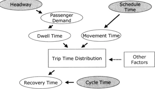
which satisfy the general agency's standards, and thus provide a minimum service quality. This means that there is no easy way to assess the operational cost and service quality with different schedule parameters and find better schedule parameters for a route. Also, the influence of a decision on one schedule parameter on the other schedule parameters is not considered in current scheduling process. Figure 2-2 shows the inter-relationships between schedule parameters, which should be considered in a general scheduling process. The gray elements are the schedule parameters that the operator can control in the scheduling process.

Passenger

Demand

Trip Time Distribution 4... Other Factors

Ac-Figure 2-2 Inter-relationships between Schedule Parameters

Vehicle trip time consists of dwell time and movement time. The dwell time will be affected by the vehicle headway since the vehicle headway determines the passenger demand at bus stops and passenger demand determines the dwell time at each stop. The vehicle movement time will be affected by the schedule time when a schedule-based holding strategy is implemented since the vehicle should not depart from the time points until the scheduled departure time. Therefore, the trip time distribution will change depending on the headway and schedule time. The half cycle time is determined by the on-time departure probability at the terminal that the transit agency wants to achieve based on the trip time distribution. The recovery time is then simply set to the difference between the half cycle time and the schedule time. In other words, the half cycle time and recovery time are determined from the desired on-time departure probability and the trip time distribution that is determined by the schedule time and

headway. Therefore, any changes in the headway and schedule time will influence decisions on other schedule parameters, specifically the half cycle time and recovery time.

The operational cost and service quality are also affected by the schedule parameters. Figures 2-3 and 2-4 show the relationship between operational cost and schedule parameters and the relationship between service quality and schedule parameters respectively.

Operational Cost

Schedule Cost

Late Trip Cost

(:Hedwa~

4-

Cyce Tim~eTrip

Time

Head ay

4*

Ccle imeDistribution

Figure 2-3 The Relationship between Operational Cost and Schedule Parameters

The operational cost includes both the schedule cost and cost of any late trip. The schedule cost during a time period is determined by the cycle time and headway, which determines the number of vehicles needed during the time period. The late trip cost is generated only if the operator has to work overtime, that is the total work time is greater than the scheduled work time. Since the total work time distribution for each piece of work consists of the trip time distributions of trips and the scheduled work time is based on the vehicle cycle time, the late trip cost will depend on the trip time distribution and cycle time.

In-vehicle

Time

Headway

Tm

Crowding

Level

Recovery

Passenger

Waiting Time

Schedule

Time

Schedule

Adherence

Figure 2-4 The Relationship between Service Quality and Schedule Parameters

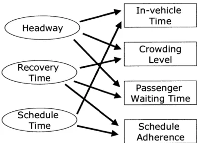
The service quality is measured by the in-vehicle time, crowding level, passenger waiting time, and schedule adherence. Passenger in-vehicle time is determined by the actual trip time. Since the trip time is affected by the headway and schedule time, the passenger in-vehicle time is affected by the headway and the schedule time. Crowding level is mainly determined by the vehicle headway since the headway determines the passenger demand at the stop. Also, by controlling the departure headway at the terminal, the recovery time can influence the passenger demand at the stop, and thus the crowding level. The passenger waiting time is determined by the headway distribution, average headway and headway variability. Average headway will be mainly affected by the schedule headway and the headway variability is affected by the recovery time. Therefore, the passenger waiting time is affected by the headway and recovery time. The schedule adherence is measured by the time arrival probability at the ending terminal and on-time departure probability at the starting terminal. The on-on-time arrival probability is determined

by the schedule time and the on-time departure probability is determined by the recovery time.

Therefore, schedule adherence is affected by the schedule time and recovery time.

In this chapter, I have reviewed the current service and operations planning process and the relationships between schedule parameters, operational cost, and service quality that will affect the decision on the schedule parameters. After deriving the relationships for a simplified route in Chapter 3, I will develop an alternative schedule parameters setting process, which incorporates the relationships between the schedule parameters, operational cost and service quality.

Chapter 3. Theoretical Analysis of Relationships between Schedule

Parameters, Operational Cost, and Service Quality

In this chapter, I derive the relationships between schedule parameters, service quality and operating cost for a general bus route having stops between a starting terminal and an ending terminal. The resulting relationships, which are developed for a simplified route with many assumptions, should be similar to those for a more complex route. By deriving the relationships for a simplified route, we can better understand the general relationships between the schedule parameters, service quality and operational cost. Before developing the relationships, the simplified route and the basic assumption made in this analysis are described. In section 3.2, the impact of schedule parameters on the trip time is developed. The inter-relationships between the schedule parameters are discussed in section 3.3, and the relationships between the operational cost and schedule parameters and the relationships between service quality and schedule parameters are developed in sections 3.4 and 3.5 respectively. In section 3.6, a revised scheduling process, which incorporates the relationships between schedule parameters, operational cost and service quality, is proposed.

3.1.

Route Description and Basic Assumption

A simple bus route with a starting terminal A, and an ending terminal B is considered

(see Figure 3-1). There are k time points (P1, P2... , Pk) between the starting and ending terminal

along the route of length d and buses run every h minutes. The basic assumptions are described below:

1. The passenger arrival rate is constant over the time period.

2. All passengers can board the first bus to arrive, i.e. the capacity constraint is not binding.

3. Successive runs are completely independent of each other.

4. The segment time (Ti) is a random variable with mean, E(Ti), and standard deviation, a(

Ti).

A PI P2 P3 -~~~~~ Pk-I Pk B

Starting nding

Terminal T1 T2 T3 Tk Tk+ Terminal

Figure 3-1 A Route with k Possible Time Points

Though these assumptions are made to simplify the problem and thus make it easy to build the relationships between schedule parameters, operational cost and service quality, they may result in an inaccurate representation of actual operating conditions. With the second assumption, we cannot consider the case that passengers may not be able to board the first bus and thus have to wait for the next bus, which can happen during the peak time for high frequency service. Thus this assumption may under-estimate the passenger waiting time by ignoring the extra time waiting for the next bus. The fourth assumption further implies that segment times are independent of each other. However, in real operations, a driver tends to drive faster in the current segment if he or she was late in the previous segment. Therefore, typical driver behavior is neglected in this assumption.

The assumption that successive runs are completely independent of each other makes it possible to schedule one run at a time and thus to derive the relationship between the schedule time and the trip time distribution. However, since this assumption implies that headway variability does not affect the overall operations much and further implies that the dwell time is not affected by headway, it cannot represent the operating condition of high frequency service. For a low frequency bus route, the headway variability does not change the passenger demand at the stop since the passenger arrives at the stop based on the schedule and thus the dwell time can be constant. For a high frequency bus route, the dwell time, which is included in trip time, .is affected by the actual headway due to different passenger demand per bus. Therefore, with this assumption, we cannot consider the randomness of dwell times in high frequency service.

From this assumption, the difference in control strategies between high frequency service and low frequency service can be discussed. For a low frequency route, the service performance is mainly measured by the schedule adherence since passengers arrive at the stop based on schedule and thus service quality is usually controlled by the schedule. However, for a high

on a bus and passengers arrive at stops randomly, service performance is mainly measured by the passenger waiting time. Thus, service quality is controlled through the headway with real time operations control strategies such as holding.

3.2.

Trip Time Distribution and Schedule Parameters

Vehicle trip time can be divided into vehicle movement time and dwell time. The dwell time will be affected by the passenger demand on the route since more time is required to handle boarding and alighting passengers as passenger demand increases. The vehicle movement time will be affected by the schedule time when schedule-based holding is implemented since the vehicle should not depart until the scheduled departure time at each time point. Therefore, the trip time, which is the sum of vehicle movement time and dwell time, will change as the schedule parameters change. In this section, I will show how the trip time distribution will change according to the changes of schedule time and headway by developing an analytical model which represents the relationship between the arrival time at a time point and the schedule departure time at the previous time point and a dwell time model which represents the relationship between dwell time and passenger load (since headway determines the passenger load, given the assumption that the passenger arrival rate is constant, it can be a relationship between dwell time and headway).

3.2.1. The Influence of Time Points and Schedule Time on Trip Time

The one-way trip time is measured from the moment the bus departs the starting terminal to the moment it arrives at the ending terminal. The trip time will be a random variable with mean E(T), and standard deviation T(T) when the schedule has a tight scheduled trip time, which is set to the minimum trip time (see Figure 3-2). In this case, there is no schedule constraint effect in the trip time, which means that vehicles leave bus stops as soon as the passenger alighting and boarding processes are completed. Since every trip time is longer than the tight scheduled trip time, the recovery time is the only way to maintain a certain level of service quality by controlling on time departure probability for the following trip.

For a low frequency bus route, the headway variability does not change the passenger demand at the stop since the passenger arrives at the stop based on the schedule. Therefore, the unconstrained trip time distribution obtained from a low frequency bus route should be free from

headway variability. However, the unconstrained trip time distribution obtained from a high frequency route will be affected by the headway distribution since the headway determines the passenger demand at the stops and thus affects the dwell time. If the headways are fairly even, the trip time distribution will be tighter while if it is not the trip time distribution will be wider. Short trip times are likely to occur with short headways and long trip times are likely to occur with long headways. Therefore the observed trip time distribution should be adjusted in order to make it free from the headway variability in case of high frequency service.

As discussed in Chapter 2, movement time is not affected by the headway while dwell time is. If we know the vehicle dwell time and movement time separately, we can modify the trip time distribution by first extracting the movement time. If we assume that the passenger arrival rate is constant over a time period, we might also assume that the dwell time of each trip will be constant if there is no headway variability. Therefore, we could get the adjusted trip time distribution, which is unaffected by the schedule time and headway, by adding the constant dwell time to the movement time distribution. However, it is more realistic to consider that the dwell time to be a random variable rather than a constant even if there is no headway variability. The dwell time distribution could be obtained from the observed data with some modification of extreme values caused by long (short) headways or with an assumption that the mean dwell time is the same but the variance is decreased if the headways are more even. The adjusted trip time distribution could be obtained by adding the movement time distribution and modified dwell time distribution.

Probability

Tmin: Minimum Trip Time

E(t): Expected Trip Time

S: Scheduled Trip Time

R: Recovery Time

C: Half Cycle Time

R(t)

Tmin S E(t) C Time

The adjusted trip time distribution should be skewed to the right with a lower bound Tmin, since it is impossible for a bus to travel along a route faster than a certain speed. However, it is possible to have a much longer than expected travel time due to traffic conditions, incidents and so on although the probability would be very low. Theoretically, the distributions having those characteristics could follow a gamma distribution (Turnquist and Bowman, 1980) or a lognormal distribution (Andersson and Scalia-Tomba, 1981).

However Figure 3-2 is unrealistic because the tight scheduled trip time is not practical due to its poor resulting service quality (low on time arrival probability) at stops along the route. Thus, the transit agency would want to have a longer scheduled trip time than the minimum. If the transit agency increases scheduled trip time without doing anything else, it will just increase the probability that vehicles are early. Moreover, for low frequency service, early arrival can be worse than late arrival since it could cause passengers to miss their targeted buses and experience very long waits. Therefore, it will not be better than the previous case of tight scheduled trip time. A holding strategy is used to prevent early departures by holding early vehicles at the time point until the scheduled departure time, thus increasing the schedule adherence. Therefore, as the scheduled trip time is increased, more holding to meet the schedule is required. In my research, I assume that schedule-based holding is implemented whenever the scheduled trip time

is longer than the minimum trip time to prevent early departures from time points.

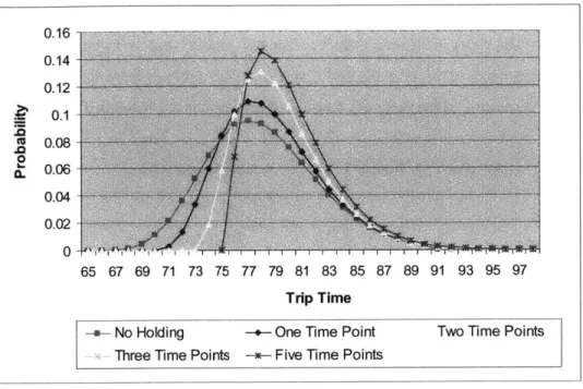
When the holding strategy is implemented, the trip time distribution is affected by the scheduled trip time. Since a vehicle which arrives early at a time point will wait till the scheduled departure time, most trips, which arrive earlier at the terminal than the scheduled arrival time without holding, will arrive close to the scheduled time with holding. However, some of these trips would not arrive at the terminal on time since there is less time to catch up with the schedule if the vehicle is delayed near the ending terminal. Therefore, the probability of late arrival at the terminal will increase with holding. When the scheduled time is increased and consequently the scheduled departure times at time points increase, the probability that a vehicle arrives at the ending terminal late will also increase. Therefore, the trip time distribution will have a longer expected trip time and tail. The trip time distribution will also be affected by the number of time points along the route. As the number of time points increases, more time is spent holding a vehicle, and thus there will be less time for catching up with schedule. Therefore, more time points will cause a higher expected trip time for a given scheduled time. In order to understand how the schedule time and holding strategy affects trip time distribution, I will derive the arrival

time distribution at the ending terminal when the holding strategy is implemented initially at only one time point (see Figure 3-3).

0 2

TI T2

Figure 3-3 Route with One Time Point

The segment time, Ti, i = 1, 2 is measured from the moment the bus leaves point i-i to

the moment the bus arrives at point i and is assumed to be a random variable with mean E(T), and standard deviation c(Ti). The vehicle arrival and departure times for point i, are Tai and Tdi respectively and scheduled departure time for point i is Si. With the assumption that every bus departs on time at the starting terminal, then So is both the actual departure time and the scheduled departure time for point 0 and is set to 0. For the ending terminal, S2 will be the

scheduled departure time for the next trip, and thus S2-Ta2 will be the recovery time. Since the scheduled departure time is set to 0, the vehicle arrival time at point 1, Tai, will be the same as T1. The vehicle arrival time at point 2, Ta2, will be the sum of the actual departure time at point 1, TdI,

and the segment running time between 1 and 2, T2. Therefore, the relationships between arrival

time and departure time between stops are:

T11= So +T = T, (3-1)

Ta2 = TI + T2 (3-2)

Since the vehicle does not depart before the scheduled departure time at time point 1, the vehicle departure time will be the scheduled departure time if the vehicle arrives earlier than the scheduled departure time or the vehicle arrival time if the vehicle is late. Note here that the dwell time is assumed to be included in the segment time.

TdI S , if Tal <S (3-3)

We can estimate the expected departure time and the variance of departure time at time point 1 as follows: E(Tdd)

= f

f,

(t)dt + S,*(I- f

D

_t

_f

The first term of E(TdI) is the expected departure time when the vehicle arrives at the time point late and the second term is the product of the probability that the vehicle arrives earlier than the scheduled departure time and the scheduled departure time itself. The expected departure time at the time point, E(Tdl), increases and the variance of Tdl decreases as the scheduled running time

increases according to the equations above.

The probability density function of departure time at time point 1, TOi can be derived as

follows:

FTj (tdl) = P{Tdl tI=}

{T

and thus

frd, (td) = F'2 (tdl) = fr., (dl) Ta S] (3-7)

Due to holding to the schedule, the probability distribution of Tdl has a discrete mass at SI.

PTdi

=

}=

PTa

Therefore, the probability distribution of Td, has a spike at Si and the distribution remains the same as the distribution of arrival time at point 1, Tai, when Tal Si.

From the relationship between the vehicle arrival time at point 2, Ta2, and the departure time at point 1, TdJ (see Equation 3-2), we can derive the expected arrival time and variance of arrival time at the ending terminal. The distribution of arrival time at the ending terminal will be the trip time distribution of the route. With the assumption that the segment running time

between points 1 and 2, T2, is independent of the departure time at time point 1, TdI, the expected

mean arrival time and variance of vehicle arrival time at the ending terminal can be derived as:

E(Ta2) = E(TdI) + E(T2)

D2 (Ta2) D2 (d]) + D2 (T2) (3-8) (3-9)

Since Tdl and T2 are assumed to be independent of each other,

obtained simply by multiplying their distributions:

fT, (td) )* fr2 (2)

their joint density function can be

Td] R SI (3-10)

Also, the joint distribution, when the vehicle arrives at time point 1 earlier than scheduled, will be the product of the probability that vehicle arrives on time at the time point 1 and the probability that T2is t2:

PTdI = S, T2 =t2}=PITd = SI I*

P{T

}=FT.,

The cumulative density function of Ta2 is:

=Sl+J IT < )ft 2 t2 dtd FT(ta2 = P{Ta2 t,2

}=FT,(St)*

}+

fr2

= FT(i)(

The probability density function of Ta2 can be derived by differentiating the cumulative density function (Equation 3-12) with respect to ta₂.

fa2 (ta) (1- Sf (t )dt) f 2 (ta2 -SI)+ fT,, (ta - t2) *J (t2)dt2 (3-13)

The first term represents the probability when the vehicles are on time at time point 1 and the second term represents the probability when they are late.